M-bias, Butterfly Bias, and Butterfly Bias with Correlated Causes – A Comment on Ding and Miratrix (2015)

1 Asymptotic biases

I used the same methodology as DM to derive the asymptotic bias in the model depicted in Figure 1. ^[1] Note that all models of DM are included in this model as special cases. If path coefficients e and f are set to 0, then we have an M-bias structure with correlated causes, if g and h are set to 0, we have a butterfly-bias structure, and if e, f, g, and h are set to zero, we have a pure M-bias structure. ^[2] Just like DM, I assume a linear structural equation model (LSEM) with completely standardized variables. Figure 1 can be expressed as the following data-generating process,

Figure 1:

Data-generating model. Disturbance terms are omitted.

where just as DM, I use A∼[0,1] to denote a random variable with mean zero and standard deviation one. All ε terms and L are assumed to be independent of each other. Just like DM, to facilitate the generation of standardized variables, I varied path coefficients in Figure 1, subject to the following constraints: (the constraints shown are not on the variances but on the path coefficients.)

Unlike DM, I allowed path coefficients to vary over a larger range, including both positive and negative signs, without any constraints that path coefficients had to be equal to each other. The only remaining point of difference to DM is that I included latent causes explicitly in the diagram, and do not used bi-directed arrows. I chose a dashed ellipse with letter L to denote the latent cause.

The asymptotic bias of the effect of T on Y in the model in Figure 1, and special cases of the model (in which certain path coefficients are set to 0), with and without adjustment on M is given in Table 1. All biases are expressed using structural coefficients of Figure 1. All biases were computed by first deriving correlations (expressed as sums and products of structural path coefficients) among variables using path-tracing rules. After correlations were obtained, I derived a regression coefficient for the relationship between T and Y, again expressed using structural path coefficients (displayed in the column labeled “Bias under no adjustment”), and a partial regression coefficient for the relationship between T and Y, conditioning on M displayed in the column labeled “Bias under adjustment on M”), using the recursive formula, as explained in e.g., Pearl [5].

Will adjustment or no adjustment yield smaller biases when evaluated under a wide range of path coefficients? To answer this question, I varied every single path coefficient in Figure 1 to take on the values −0.9,−0.6,−0.3,−0.1,0,0.1,0.3,0.6,0.9 and formed every possible combination, subject to the constraints expressed above, yielding a total of 26, 828, 109 models. For the two special cases of M-bias with correlated causes and butterfly-bias, I varied the non-zero path coefficient with even smaller intervals, ranging from from –0.9 to 0.9 in increments of 0.15 (yielding 13 unique levels), and formed all possible combinations, for a total of 3, 521, 961 combinations for the M-bias structure with correlated causes, and 2,614, 937 combinations for the butterfly-bias structure). These combinations were evaluated separately. For every model, I computed bias with and without adjustment, and formed a difference of absolute biases between the two models. ^[3] Numerical summaries of biases for all models are given in Table 2, and histograms of the difference in absolute bias are presented in Figure 2.

Figure 2:

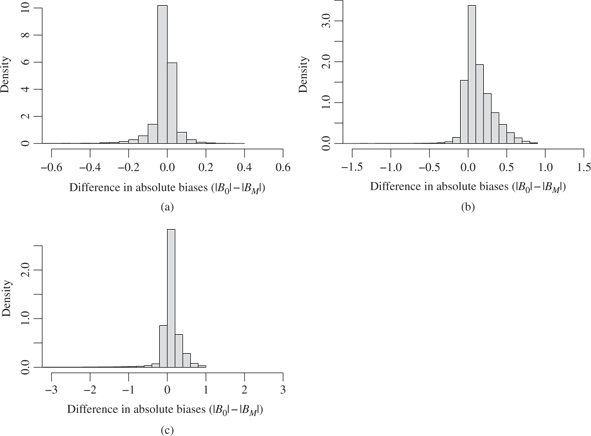
Density estimate of difference in absolute biases with or without adjustment on M in model in Figure 2. M-bias model with correlated causes is labeled (a), butterfly-bias model is (b), and full model is (c). Axes are not constant across graphs. B0 is bias without adjustment on M, and BM is bias with adustment on M.

Considering first the special case of M-bias with correlated causes (model in Figure 1 with e=f=0), we can observe that the difference in absolute biases is almost symmetrical (see Figure 2(a), implying that over the observed parameter space, adjustment is just as likely to increase as to decrease bias. Numerically, in 56% of all cases bias was larger in the unadjusted model. In 81% of all cases, the two biases were virtually identical to each other, with differences smaller than |0.05| on the raw bias metric. ^[4] In 13% of all cases, the bias of the adjusted model was at least 0.05 larger, with an average increase in absolute bias of 0.12, and in 6% of all cases, bias was at least 0.05 larger in the unadjusted model, with an average bias of 0.10. This confirms the conjecture by Pearl [7], that in the case of M-bias with correlated causes, it can be either helpful or hurtful to adjust with approximately equal probability. If anything, the results slightly caution against adjustment, as indicated by the slight imbalance in the distribution.

In the special case of the butterfly-bias (when g=h=0), I replicated the results of DM (but over a wider parameter range), and also observed that in a vast majority of cases, adjustment on M was preferable, as indicated in the skewed distribution of the difference in absolute bias, shown in Figure 2(b).

Numerically, in 85% of all cases was adjustment preferable over the unadjusted estimator. In 32.5% of all cases, the two biases were virtually identical, with differences smaller than |0.05|. In only 5% of all cases, the bias of the adjusted model was at least 0.05 larger, with an average increase in absolute bias of 0.17, and in 62.5% of all cases, bias was at least 0.05 larger in the unadjusted model, with an average bias of 0.23. This confirms the findings of DM that adjustment is virtually always better in the case of the butterfly-bias.

Finally, I evaluated the full model which extended the butterfly-bias structure to include correlated causes U and W. This is the model with the least constraints, and arguably the most realistic. As shown in Figure 2(c), the distribution of absolute difference in biases, was slightly skewed to the right, indicating that there were more situations in which adjustment lowered bias. However, while there were fewer cases in which adjustment increased bias, when it did, the magnitude of the increase was higher. Numerically, in 69% of all cases was adjustment preferable over the unadjusted estimator. In 41% of all cases, the two biases were virtually identical, with differences smaller than |0.05|. In only 8% of all cases, the bias of the adjusted model was at least 0.05 larger, with an extremely large average increase in absolute bias of 2.42. ^[5] In 50% of all cases, bias was at least 0.05 larger in the unadjusted model, with an average bias of 0.23. What we observe in this model is that conditioning on a pre-treatment variable like M in Figure 1 is likely going to decrease bias, confirming the results of DM, but in cases in which it does not, bias may increase substantially, a warning also spelled out by Pearl [7].

2 Conclusion

Some of the conclusions of DM can be confirmed, others must be slightly qualified, once negative correlations, and deviations from equal magnitude of path coefficients, are being considered. In agreement with Pearl [7], I also do not believe that positive correlations are more frequent in real data, and that a full exploration of the parameter space is necessary, as was provided here. Considering this larger and more complete parameter space, M-bias with correlated causes appears to be equally likely to increase or decrease bias upon adjustment, butterfly-bias seems to be primarily decreased by adjustment, and in the model with the least constraints considered in this paper, bias is also more generally attenuated, with the caveat that if it is not, the induced bias tends to be large.

How should these results inform applied researchers? First, it is important to remind ourselves that the models in DM and the extended versions presented here are still toy models that most likely will not be representative of real research situations. I argue that in applied research it is still preferable to rely on methods that are guaranteed to minimize bias (under assumptions expressed, e.g., in a DAG), such as the back-door criterion [4], the adjustment criterion [8], or the disjunctive cause criterion [9]. All of these criteria rely on making certain assumptions, and are thus not “model-free.” The importance of such model-based decision-making and the issue of conditioning on colliders as in the M-bias structure has recently also been recognized in the domain of missing data analysis, where conventional wisdom dictated that all available covariates should always be used in the estimation of parameters in the presence of missing data. That this is not generally correct has been shown by several authors [10–13].

If none of the criteria mentioned above are fulfilled, but may be approximated by conditioning on a variable with both bias-inducing and bias-reducing properties, researchers may attempt to endow their theoretical models with quantitative assumptions about strength of assumed relationships, and then use the methods outlined in Chen and Pearl [6], Ding and Miratrix [1], or this paper, to determine whether inclusion in the adjustment set is likely to increase or decrease overall bias. These so-called signed graphs come with additional assumptions e.g., monotonicity of effects, and are described by VanderWeele and Robins [14].

I readily agree that the model-free approach of including everything that is a pre-treatment covariate, favored by DM and others, may in many instances yield decreases in bias, however with one caveat: one would never know if the data at hand are one of those instances in which bias is increased through adjustment. Such instances would occur with 5–13% chance in the models considered above. Maybe a small chance, but why take it, if one is able to think about and encode the underlying causal assumptions, and thus potentially identify (and avoid) these cases?

I would like to finish this paper with a small anecdote. Recently, I was involved in a project with applied colleagues who were interested in the causal effect of chronic pain on depression. We spent many hours discussing which of the many variables that preceded chronic pain we should adjust on. We did draw a causal graph and we thought many hours about the structure among our variables of interest and the potential covariates. In the end, we did use all pre-treatment covariates to adjust on, thus in practice following the recommendation of DM. However, I still believe that the process of thinking about the structure was worthwhile (even though time-consuming), because it not only deepened our appreciation of the theoretical intricacies of the covariates, but also guarded us against adjusting on variables that could have increased bias, something that we would not have been able to do if we automatically adjusted on everything.

References

1. DingP, MiratrixLW. To adjust or not to adjust? Sensitivity analysis of m-bias and butterfly-bias. J Causal Inference2015;3:41–57.10.1515/jci-2013-0021Search in Google Scholar
2. RubinDB. The design versus the analysis of observational studies for causal effects: parallels with the design of randomized trials. Stat Med2007;26:20–36.10.1002/sim.2739Search in Google Scholar PubMed
3. PearlJ. Myth, confusion, and science in causal analysis. Technical Report R-348, University of California, Los Angeles, CA. Available at: http://ftp.cs.ucla.edu/pub/stat_ser/r348.pdf, 2009.Search in Google Scholar
4. PearlJ. Remarks on the method of propensity scores. Stat Med2009;28:1415–16.10.1002/sim.3521Search in Google Scholar PubMed
5. PearlJ. Linear models: A useful “microscope” for causal analysis. J Causal Inference2013;1:155–70.10.1515/jci-2013-0003Search in Google Scholar
6. ChenB, PearlJ. Graphical tools for linear structural equation modeling. Technical Report R-432, Department of Computer Science, University of California, Los Angeles, CA, forthcoming, Psychometrika. Available at: http://ftp.cs.ucla.edu/pub/stat_ser/r432.pdf, 2014.Search in Google Scholar
7. PearlJ. Comment on Ding and Miratrix:“to adjust or not to adjust?”J Causal Inference2015;3:59–60.10.1515/jci-2015-0004Search in Google Scholar
8. ShpitserI, VanderWeeleTJ, RobinsJM. On the validity of covariate adjustment for estimating causal effects. In: UAI 2010, Proceedings of the twenty-sixth conference on uncertainty in artificial intelligence, Catalina Island, CA, USA, July 8–11, 2010: 527–536.Search in Google Scholar
9. VanderWeeleTJ, ShpitserI. A new criterion for confounder selection. Biometrics2011;67:1406–13.10.1111/j.1541-0420.2011.01619.xSearch in Google Scholar PubMed PubMed Central
10. MohanK, PearlJ, TianJ. Graphical models for inference with missing data. In: C. Burges, L. Bottou, M. Welling, Z. Ghahramani, K. Weinberger, editors. Advances in neural information processing systems, 26, 2013: 1277–85. Available at: http://papers.nips.cc/paper/4899-graphical-models-for-inference-with-missing-data.pdf.Search in Google Scholar
11. PearlJ, MohanK. Recoverability and testability of missing data: Introduction and summary of results. Technical Report R-417. Department of Computer Science, University of California, Los Angeles, CA, 2014. Available at: http://ftp.cs.ucla.edu/pub/stat_ser/r417.pdf.10.2139/ssrn.2343873Search in Google Scholar
12. ThoemmesF, MohanK. Graphical representation of missing data problems. Struct Equ Modeling2015:1–13.Search in Google Scholar
13. ThoemmesF, RoseN. A cautious note on auxiliary variables that can increase bias in missing data problems. Multivar Behav Res2014;49:443–59.10.1080/00273171.2014.931799Search in Google Scholar PubMed
14. VanderWeeleTJ, RobinsJM. Signed directed acyclic graphs for causal inference. J R Stat Soc Ser B (Stat Methodol)2010;72:111–27.10.1111/j.1467-9868.2009.00728.xSearch in Google Scholar PubMed PubMed Central
©2015 by De Gruyter
Articles in the same Issue
- Frontmatter
- Balancing Score Adjusted Targeted Minimum Loss-based Estimation
- Surrogate Endpoint Evaluation: Principal Stratification Criteria and the Prentice Definition
- A Causal Perspective on OSIM2 Data Generation, with Implications for Simulation Study Design and Interpretation
- Parameter Identifiability of Discrete Bayesian Networks with Hidden Variables
- The Bayesian Causal Effect Estimation Algorithm
- Propensity Score Analysis with Survey Weighted Data
- Comment
- Reply to Professor Pearl’s Comment