Design and Analysis of Experiments in Networks: Reducing Bias from Interference
-
Dean Eckles

 ,
Brian Karrer
,
Brian Karrer

Abstract
Estimating the effects of interventions in networks is complicated due to interference, such that the outcomes for one experimental unit may depend on the treatment assignments of other units. Familiar statistical formalism, experimental designs, and analysis methods assume the absence of this interference, and result in biased estimates of causal effects when it exists. While some assumptions can lead to unbiased estimates, these assumptions are generally unrealistic in the context of a network and often amount to assuming away the interference. In this work, we evaluate methods for designing and analyzing randomized experiments under minimal, realistic assumptions compatible with broad interference, where the aim is to reduce bias and possibly overall error in estimates of average effects of a global treatment. In design, we consider the ability to perform random assignment to treatments that is correlated in the network, such as through graph cluster randomization. In analysis, we consider incorporating information about the treatment assignment of network neighbors. We prove sufficient conditions for bias reduction through both design and analysis in the presence of potentially global interference; these conditions also give lower bounds on treatment effects. Through simulations of the entire process of experimentation in networks, we measure the performance of these methods under varied network structure and varied social behaviors, finding substantial bias reductions and, despite a bias–variance tradeoff, error reductions. These improvements are largest for networks with more clustering and data generating processes with both stronger direct effects of the treatment and stronger interactions between units.
1 Introduction
Many situations and processes of interest to scientists involve individuals interacting with each other, such that causes of the behavior of one individual are also indirect causes of the behaviors of other individuals; that is, there are peer effects or social interactions [1]. Likewise, in applied work, the policies considered by decision-makers often have many of their effects through the interactions of individuals [2]. Examples of such cases are abundant. In online social networks, the behavior of a single user explicitly and by design affects the experiences of other users in the network. If an experimental treatment changes a user’s behavior, then it is reasonable to expect that this will have some effect on their friends, a perhaps smaller effect on their friends of friends, and so on out through the network. In an extreme case, treating one individual could alter the behavior of everyone in the network.
To see the challenges this introduces, consider what is, in many cases, a primary quantity of interest for experiments in networks – the average treatment effect (ATE) of applying a treatment to all units compared with applying a different (control) treatment to all units.[1] Let
where
Rather than substituting other strong assumptions about interference that may result in point identifying
We do not consider all possible designs and analysis, but limit this work to some relatively general methods for each. We consider experimental designs that assign clusters of vertices to the same treatment; this is graph cluster randomization [16]. Since the counterfactual situations of interest involve all vertices being in the same condition, the intuition is that assigning a vertex and vertices near it in the network into the same condition, the vertex is “closer” to the counterfactual situation of interest.[5] For analysis methods, we consider methods that define effective treatments such that only units that are effectively in global treatment or global control are used to estimate the ATE. For example, an estimator for the ATE might only compare units in treatment that are surrounded by units in treatment with units in control that are surrounded by units in control. The intuition is that a unit that meets one of these conditions is again “closer” to the counterfactual situation of interest.
The rest of the paper is structured as follows. We briefly review some related work on experiments in networks. Section 2 presents a model of the process of experimentation in networks, including initialization of the network, treatment assignment, outcome generation, and analysis. This formalization allows us to develop theorems giving sufficient conditions for bias reduction. To develop further understanding of the magnitude of the bias and error reduction in practice, Section 3 presents simulations using networks generated from small-world models and then degree-corrected blockmodels. While our theoretical sufficient conditions for bias reduction are somewhat restrictive, the simulations include data generating processes that do not meet these sufficient conditions yet still show substantial bias and error reductions, demonstrating that our alternative design and analysis approaches remain useful far outside the range of the theorems.
We find that graph cluster is capable of dramatically reducing bias compared to independent assignment without adding “too much” variance. The benefits of graph cluster randomization are larger when the network has more local clustering and when social interactions are strong. If social interactions are weak or the network has little local clustering, then the benefits of the more complex graph-clustered design are reduced. Finally, we found larger bias and error reductions through design than analysis: analysis strategies using neighborhood-based definitions of effective treatments do further reduce bias, but often at a substantial cost to precision such that the simple estimators were preferable in terms of error. No combination of design and analysis is expected to work well across very different situations, but these general insights from simulation can be a guide to practical real-world experimentation in the presence of peer effects.
1.1 Related work
Much of the literature on interference between units focuses on situations where there are multiple independent groups, such that there are interactions within, but not between, groups, (e.g., [6, 7, 8, 17]). Some more recent work has studied interference when the analyst may only observe a single, connected network [9, 14, 15, 16, 18, 19, 22], where this between-groups independence structure cannot be assumed. Walker and Muchnik [23] review some of this work, including a previous version of this paper.
Two features are common to much of this growing body of work on interference in networks. First, most work has focused on assuming restrictions on the extent of interference (e.g., vertices are only affected by the number of neighbors treated) and then deriving results for designs and estimators motivated by these same assumptions. Aronow and Samii [15] give unbiased estimators for ATEs under these assumptions and derive variance estimators. Also using these assumptions, Ugander et al. [16] show that graph cluster randomization puts more vertices in the conditions required for these estimators, such that the variance of these estimators is bounded for certain types of networks, such that the asymptotic variance is
Second, much of the related work has focused on detecting or estimating effects of peer assignments on ego outcomes; that is, estimating the magnitude of local interference (i.e., exogenous peer effects, indirect effects, spillovers) rather than estimating a global ATE. Again, one exception is Choi [21], which considers a contrast between global control (or treatment) and whatever treatment vector was actually observed.
The present work explicitly considers realistic data generating processes that violate these restrictive assumptions. That is, in contrast to prior work, we evaluate design and analysis strategies in the absence of assumptions that deliver particular desirable properties (e.g., unbiasedness, asymptotic consistency). Instead, we settle for reducing the bias and error of our inevitably biased estimators.
2 Model of experiments in networks
We consider experimentation in networks as consisting of four phases: (i) initialization, (ii) treatment assignment, (iii) outcome generation, and (iv) estimation. A single run through these phases corresponds to a single instance of the experimental process. Treatment assignment embodies the experimental design, and the estimation phase embodies the analysis of the network experiment. These same phases, shown in Figure 1, are implemented in our simulations in which we instantiate this process many times.
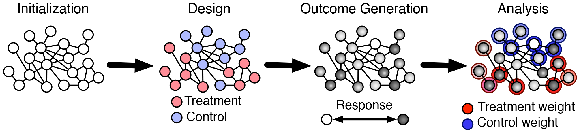
Model of the network experimentation process, consisting of (i) initialization, which generates the graph and vertex characteristics, (ii) design, which determines the randomization scheme, (iii) outcome generation, which observes or simulates behavior, and (iv) analysis, which constructs an estimator. We examine the bias and variance of treatment effect estimators under different design and analysis methods for varied initialization and outcome generation processes.
2.1 Initialization
Initialization is everything that occurs prior to the experiment. This includes network formation and the processes that produce vertex characteristics and prior behaviors. In some cases, we may regard this initialization process as random, and so wish to understand design and analysis decisions averaged over instances of this process; for example, we may wish to average over a distribution of networks that corresponds to a particular network formation model. In the simulations later in this paper, we generate networks from small-world models [24] and degree-corrected blockmodels [25]. In other cases, we may regard the outcome of this process as fixed; for example, we may be working with a particular network and vertices with particular characteristics, which we wish to condition on in planning our design and analysis.
When initialization is complete, we have a particular network
2.2 Design: Treatment assignment
The treatment assignment phase creates a mapping from vertices to treatment conditions. We only consider a binary treatment here (i.e., an “A/B” test), so the mapping is from vertex to treatment or control. Treatment assignment normally involves independent assignment of units to treatments, such that one unit’s assignment is uncorrelated with other units’ assignments.[7] In this case, each unit’s treatment is a Bernoulli random variable
with probability of assignment to the treatment
The present work evaluates treatment assignment procedures that produce assignments with network autocorrelation. While many methods could produce such network autocorrelation, we work with graph cluster randomization, in which the network is partitioned into clusters and those clusters are used to assign treatments. Let the vertices be partitioned into
In standard graph cluster randomization, as presented by Ugander et al. [16], treatments are assigned at the cluster level, where each cluster
For some estimands and analyses, assigning all vertices in a cluster to the same treatment can make it impossible for some vertices to be observed with, e.g., some particular number of treated peers. This can violate the standard requirement for causal inference that all units have positive probability of assignment to all conditions being compared positivity, cf. [15]. For this reason, it can be desirable to use an assignment method that allows for some vertices to be assigned to a different treatment than the rest of its cluster; we describe such a modification in Appendix A.1.
Graph cluster randomization could be applied to any mapping
2.3 Outcome generation and observation
Given the network (along with vertex characteristics and prior behavior) and treatment assignments, some data generating process produces the observed outcomes of interest. In the context of social networks, typically this is the unknown process by which individuals make their decisions. In this work, we consider a variety of such processes. For our simulations, we use a known process meant to simulate decisions, in which units respond to others’ prior behaviors. Doing so allows us to understand the performance of varied design and analysis methods, measured in terms of estimators’ bias and error, under varied (although simple) decision mechanisms. Before considering these processes themselves, we consider outcomes as a function of treatment assignment.
2.3.1 Treatment response assumptions
In the following presentation, we use the language of “treatment response” assumptions developed by Manski [14] to organize our discussion of outcome generation. Consider vertices’ outcomes as determined by a function from the global treatment assignment
We then observe
We can, as we have done above, continue to write
If vertices’ outcomes are not affected by others’ treatment assignment, then SUTVA is true. Perhaps more felicitously, Manski [14] calls this assumption individualistic treatment response (ITR). Under ITR we could then consider vertices as having a function from only their own assignment to their outcome:
One way for this assumption to hold is if the vertices do not interact.[9] This specification of
ITR is a particular version of the more general notion of constant treatment response (CTR) assumptions [14]. More generally, a CTR assumption involves establishing equivalence classes of treatment vectors by defining a function
for any two global assignments
Other CTR assumptions have been proposed that allow for some interference. Aronow and Samii [15] simply posit different restrictions on this function, such as that a vertex’s outcome only depends on its assignment and its neighbors’ assignments. This neighborhood treatment response (NTR) assumption has that, for any two global assignments
where
2.3.2 Implausibility of tractable treatment response assumptions
How should we select an exposure model? Aronow and Samii [15] suggest that we “must use substantive judgment to fix a model somewhere between the traditional randomized experiment and arbitrary exposure models”. However, it is unclear how substantive judgement can directly inform the selection of an exposure model for experiments in networks – at least when the vast majority of vertices are in a single connected component. Interference is often expected because of social interactions (i.e., peer effects) where vertices respond to their neighbors’ behaviors: in discrete time, the behavior of a vertex at
We consider a dynamical model with discrete time steps in which a vertex’s behavior at time
where
Together with the graph
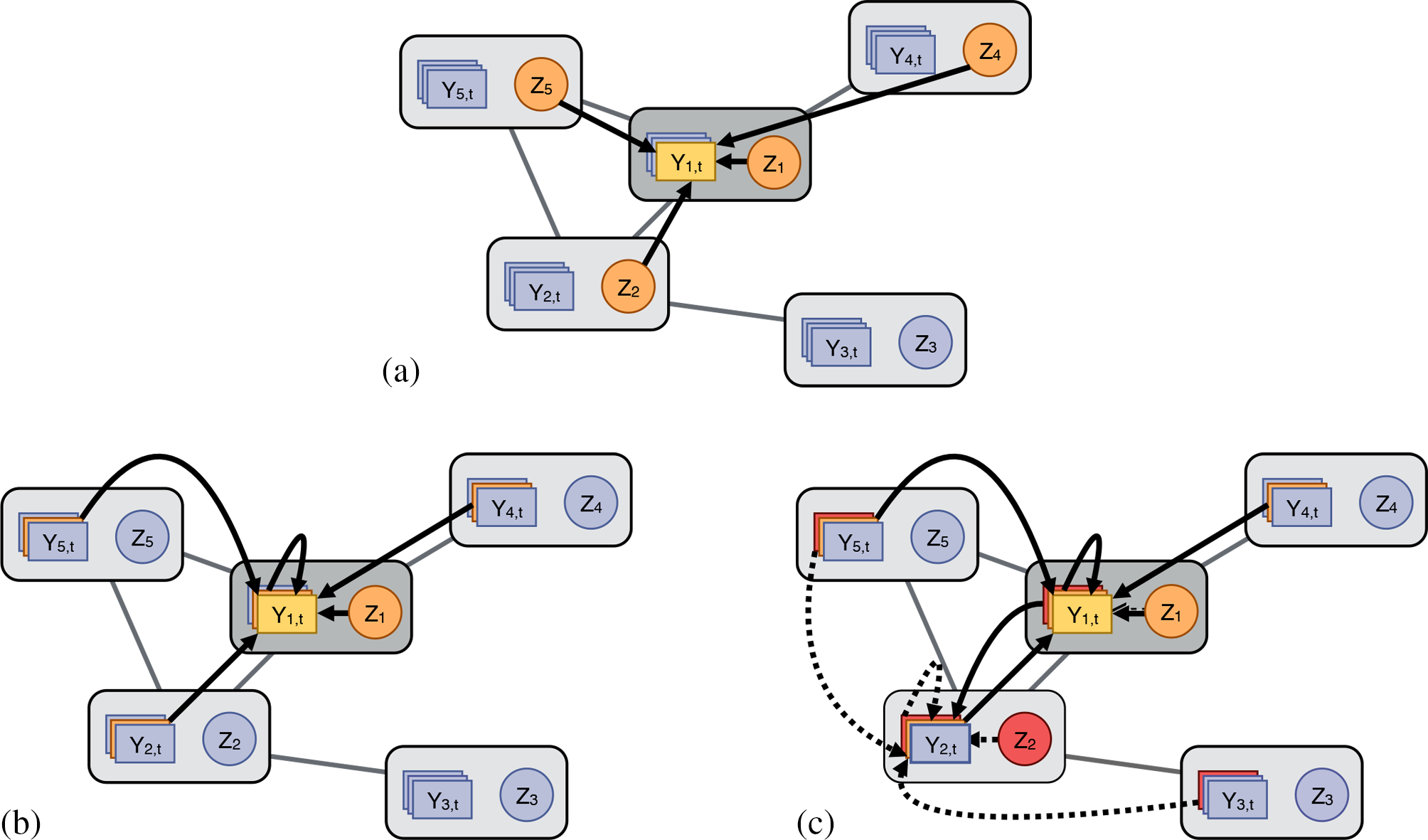
Varieties of interference illustrated in a small social network. (a) Interference under the neighborhood treatment response (NTR) assumption, where the response of vertex 1 at time t (light orange) depends on the treatments of its neighbors and itself (dark orange). (b) Interference due to social interactions (i.e., peer effects, social contagion), where the response of vertex 1 at time t depends on its own treatment
2.3.3 Utility linear-in-means
Many familiar models are included in the above outcome generating process. To make this more concrete, clarify the relationship to work on graphical games, and for our subsequent simulations, we consider a model in which a vertex’s behavior is a stochastic function of the mean of neighbors’ prior behaviors, so that behavior at some new time step
where
This can be interpreted as a simple noisy best response or best reply model [31], when vertices anticipate neighbors taking the same action in the present round as they did in the previous round. In particular, we can interpret
2.4 Analysis and estimation
We focus on the ATE (the average treatment effect;
There are many options available for estimating the ATE. For example, if the relevant network is completely unknown or if peer effects are not expected, then one might use estimators for experiments without interference, such as a simple difference-in-means between the outcomes of vertices assigned to treatment and control. To clarify the sources of error in estimation, we begin with the population analogs of these quantities – i.e., the associated estimands defined with respect to the observed and unobserved potential outcomes – and return to the estimators themselves in Section 2.4.3. Consider the simple difference-in-means estimand
where the
We index these quantities by both the definition of effective treatments (ITR for “individualistic treatment response”, as in Section 2.3.1) and the experimental design
When a vertex’s outcome depends on the treatment assignments of others, these estimands need not equal the quantities of interest. That is, they can suffer from some estimand bias (or model bias), such that
2.4.1 Bias reduction through design
We are now equipped to elaborate on the intuition that graph cluster randomization puts vertices in conditions “closer” to the global treatments of interest and thereby reduces bias in estimates of average treatment effects, even if a vertex’s outcome depends on the global treatment vector.
Theorem 2.1
Assume we have a linear outcome model for all vertices
Then for any mapping of vertices to clusters
Proof
Using the linear model for
for this outcome model. Under graph cluster randomization,
Then under independent assignment,
Because
To clarify this further, let’s consider the relative bias defined by
Assume that there are
In Appendix A.2, we derive similar intuitions from an alternative graph cluster randomization that preserves balance between the sizes of the treatment and control group. There graph cluster randomization no longer always achieves bias reduction for every clustering over independent assignment, but meaningful bias reduction is again possible and again depends on how the clustering captures
This linear outcome model, which has
The closed form solution for
where
To be clear, the linearity and monotonicity assumption made in Theorem 2.1 are restrictive assumptions, but it is important to note that they are sufficient, rather than necessary, conditions for graph cluster randomization to reduce bias. The probit utility linear-in-means model introduced in Section 2.3.3 and used for the later simulations will not meet the conditions of the theorem, yet still shows bias reduction.
2.4.2 Bias reduction through analysis
Definitions of effective treatments other than ITR correspond to different estimands. In particular, we can incorporate assumptions about effective treatments into eq. (1). Let
be the mean outcome for the global treatment
as our revised estimand for the ATE.[15] If the effective treatment definition is correct, then this estimand will also be the global ATE. As with the ITR assumption, we can again describe the estimand bias that occurs when effective treatments are incorrectly specified. For some global treatment vector
where
Considering two specifications of effective treatments allows us to elaborate on the intuition that using a finer specification of effective treatments will reduce bias by comparing only vertices that are in conditions “closer” to the global treatments of interest. For example, the NTR assumption corresponds to finer effective treatments than the ITR assumption. We can also relax the NTR assumption to a fractional
To show sufficient conditions for bias reduction, we define the following generalization of this relationship among definitions of effective treatments. Consider functions
Definition 2.2
If we have two such functions
Theorem 2.3
Let
Proof.
Given in Appendix A.3.
What about the combination of a design using graph cluster randomization with an analysis using these neighborhood-based estimands? As we show in Appendix A.3, similar arguments apply if
2.4.3 Estimators
We now briefly discuss estimators for the estimands considered above. First, we can estimate
Note that these estimators are again indexed by the effective treatment used (i.e., ITR), but, unlike the estimands, they are not indexed by the design, though the design determines their distribution. We additionally distinguish these estimators by the weighting used (discussed below), identifying the simple (i.e., unweighted) means with
where we have
This estimator will only be unbiased for the corresponding estimand
Observed effective treatments can be made unconfounded by conditioning on the design [15] or sufficient information about the vertices. The experimental design determines the probability of assignment to an effective treatment
The bias of this Hajek estimator for eq. (13) is not zero, but it is typically small and worth the variance reduction, cf. [15].
Beyond bias, we also care about the variance of the estimator as well. Estimators making use only of vertices with all neighbors in the same condition will suffer from substantially increased variance, both because few vertices will be assigned to this effective treatment and because the weights in the Hajek estimator will be highly imbalanced. This could motivate borrowing information from other vertices, such as by using additional modeling or, more simply, through relaxing the definition of effective treatment, such as by using the fractional relaxation of the NTR assumption (FNTR).
The most appropriate effective treatment assumption to use for the analysis of a given experiment is not clear a priori. We will consider estimators motivated by two different effective treatments in our simulations.
3 Simulations
In order to evaluate both design and analysis choices, we conduct simulations that instantiate the model of network experiments presented above. First, graph cluster randomization puts more vertices into positions where their neighbors (and neighbors’ neighbors) have the same treatment; this is expected to produce observed outcomes “closer” to those that would be observed under global treatment. Second, estimators using fractional neighborhood treatment restrict attention to vertices that are “closer” to being in a situation of global treatment. Third, weighting using design-based propensity scores adjusts for bias resulting from associations between propensity of being in an effective treatment of interest and potential outcomes. Each of these three changes to design and analysis is expected to reduce bias, potentially at a cost to precision. Under some conditions, we have shown above that these design and analysis methods reduce (or at least do not increase) bias for the ATE. The goal of these simulations then is to characterize the magnitude of this bias reduction, weigh it against increases in variance, and do so specifically under circumstances that do not meet the given sufficient conditions for the theoretical results.
For each run of the simulation, we do the following. First, we construct a small world network with
For graph cluster randomization, we use
We initialize
Finally, for each simulation, we compute three estimates of the ATE. The individual unweighted estimator (or difference-in-means estimator)
We run each of these configurations 5,000 times. We estimate the true ATE with simulations in which all vertices are put in treatment or control. Each configuration is run 5,000 times for the global treatment case and 5,000 times for the global control case.[20] Our evaluation metrics are bias and root mean squared error (RMSE) of the estimated ATE.
3.1 Design
First we examine the bias and mean squared error of the estimated ATE for designs using graph cluster randomization compared with independent randomization. In both cases we use the difference-in-means estimator
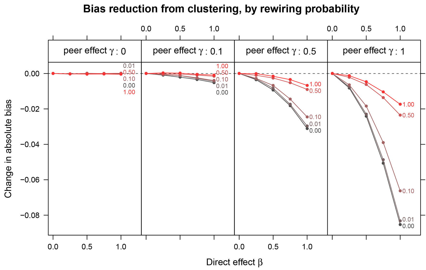
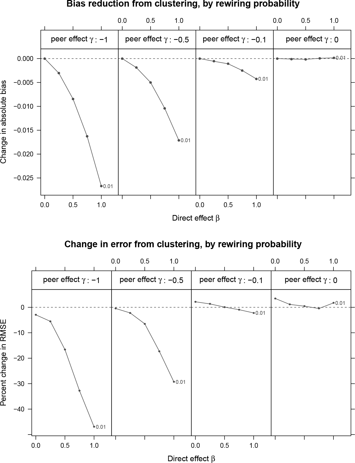
Change in bias due to clustered random assignment as a function of the direct effect of the treatment
Reduction in bias can come with increases in variance, so it is worth evaluating methods that reduce bias also by the effect they have on the error of the estimates. We compare RMSE, which is increased by both bias and variance, between graph cluster randomization and independent assignment in Figure 4. In some cases, the reduction in bias comes with a significant increase in variance, leading to an RMSE that is either left unchanged or even increased. However, in cases where the bias reduction is large, this overwhelms the increase in variance, such that graph cluster randomization reduces not only bias but also RMSE substantially. For example, with substantial clustering (
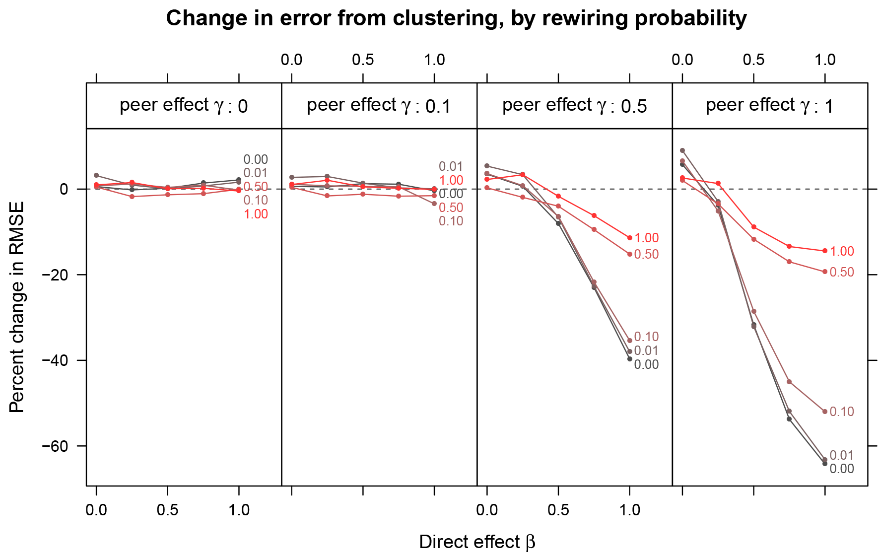
Percent change in root-mean-squared-error (RMSE) from clustered assignment for small world networks. While in some cases graph cluster randomization increases RMSE, in other cases (when bias reduction is large), it quite substantially reduces RMSE.
3.2 Design and analysis
In addition to changes in design, we can also use analysis methods intended to account for interference. We utilize the fractional neighborhood exposure model, which means we only include vertices in the analysis if at least three-quarters of their friends were given the same treatment assignment.[21] With this neighborhood exposure model, we consider using propensity score weighting, which corresponds to the Hajek estimator, or ignoring the propensities and using unweighted difference-in-means. The second estimator has additional bias due to neglecting the propensity-score weights.
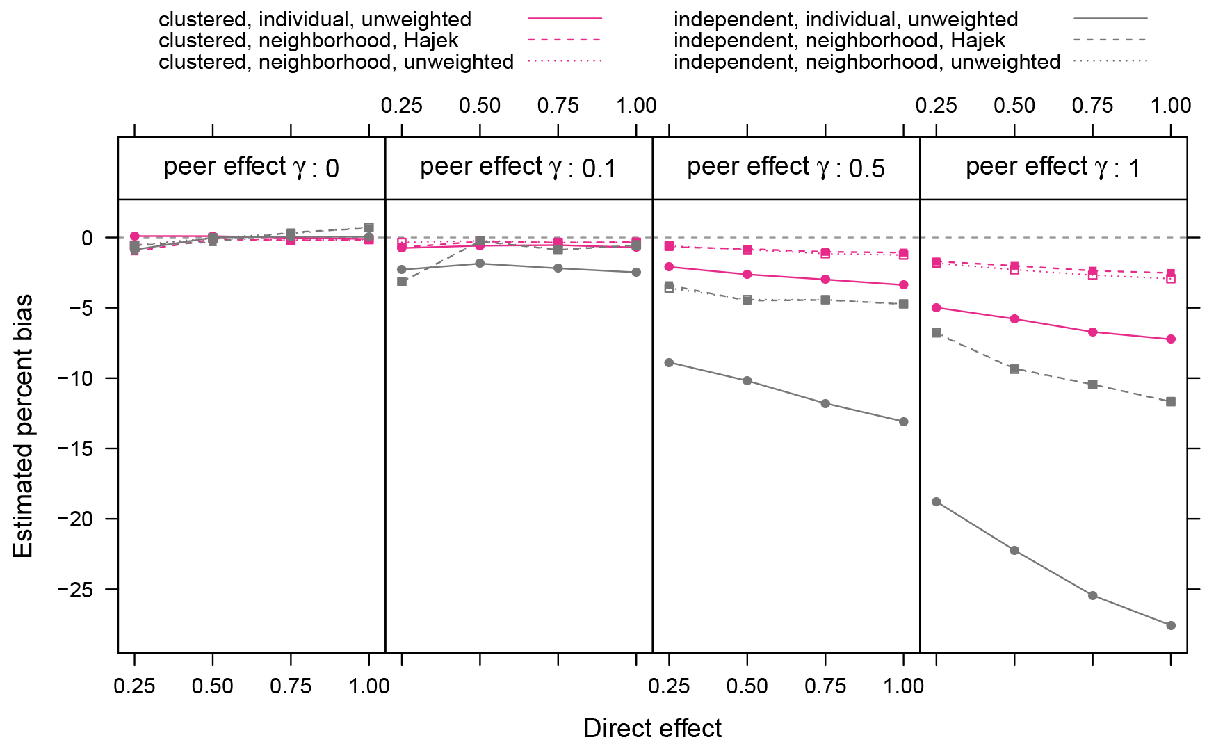
Relative bias in ATE estimates for different assignment procedures, exposure models, and estimation methods. The most striking differences are between the assignment procedures, though the neighborhood exposure model also reduces bias (at the cost of increased variance – see Figure 6). Relative bias is not defined when the true value is zero, so we exclude simulations with the direct effect
Figure 5 shows several combinations of design randomization procedure, exposure model, and estimator. We see that using a neighborhood-based definition of effective treatments further reduces bias, while the impact of using the Hajek estimator is minimal.
The low impact of the Hajek estimator follows understandably from the fact that small-world graphs do not exhibit any notable variation in vertex degree, which is the principle determinant of the propensities used by the Hajek estimator. Thus, for small-world graphs the weights used by the Hajek estimator are very close to uniform. With more degree heterogeneity expected in real networks, the weighting of the Hajek estimator will be more important, especially when these heterogeneous propensities are highly correlated with behaviors. In general, however, the change in bias from adjusting the analysis are not as striking as those from changes due to the experimental design.
Using the neighborhood exposure model means that the estimated average treatment effect is based on data from fewer vertices, since many vertices may not pass the a priori condition. So the observed modest changes in bias come with increased variance, as reflected in the change in RMSE compared with independent assignment without using the exposure condition (Figure 6).
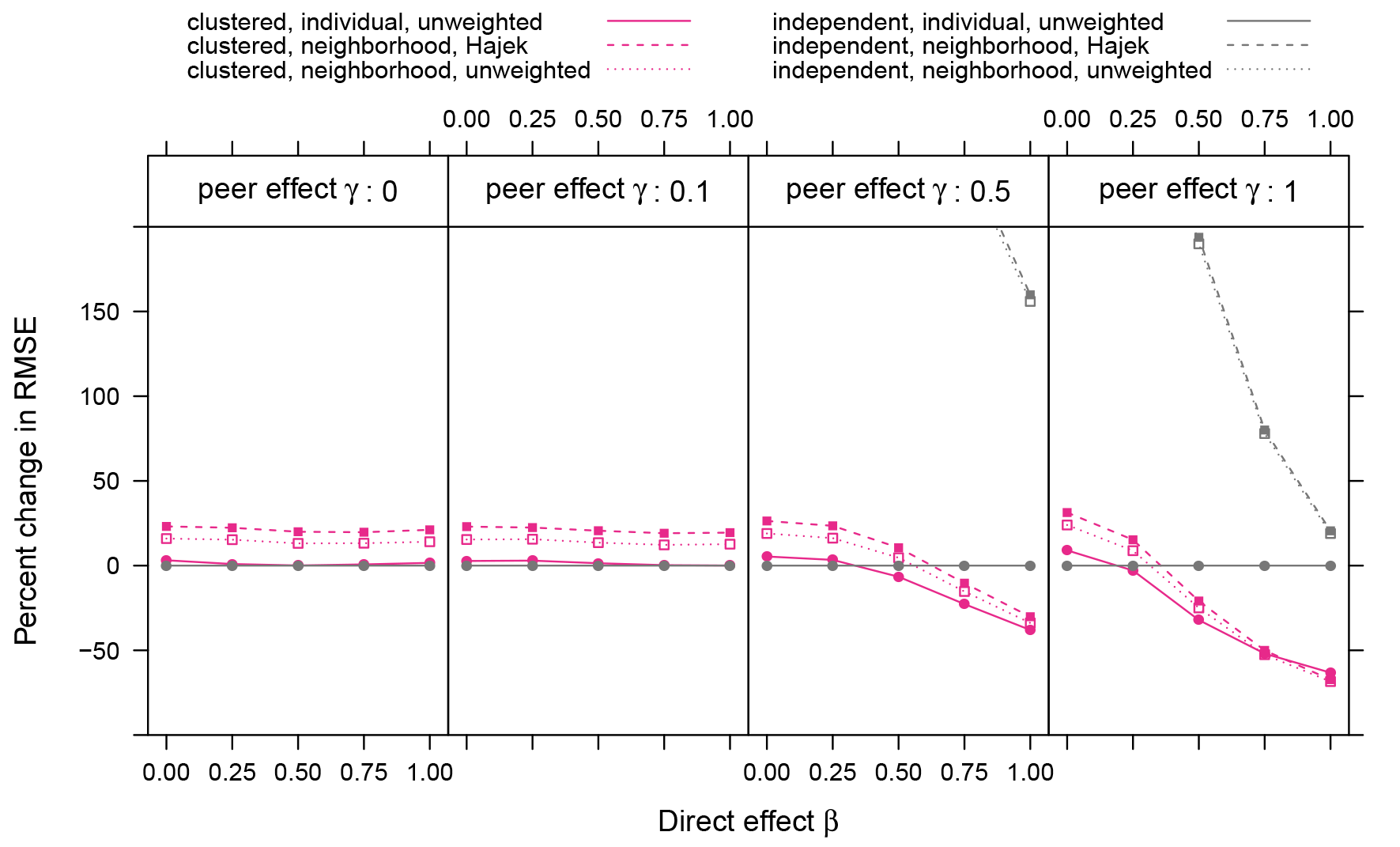
Percent change in root-mean-squared-error (RMSE) compared with independent assignment with the simple difference-in-means estimator. Using the neighborhood condition with independent assignment results in large increases in variance: for the two smaller values of
3.3 Results with stochastic blockmodels
As a check on the robustness of these results to the specific choice of network model, we also conducted simulations with a degree-corrected block model (DCBM) [25], which provides another way to control the amount of local clustering in a graph and to produce more variation in vertex degree than is possible with small world networks.
In each simulation, the network is generated according to a DCBM with 1,000 vertices and 10 communities. We present results for a subset of the parameter values used with the small-world networks. Instead of varying the rewiring probability
Figure 7 displays the change in bias and error that results from graph cluster randomization in these simulations. Again, while small on the absolute scale, the observed bias reductions are, with the exception of cases where there are no direct effects, reducing bias by at least 20%. This is reflected in the RMSE reduction results, which include the added error due to variance from graph cluster randomization. The bias and error reduction with the DCBM networks is not as large, for the same values of other parameters, as with the small world networks. We interpret this as a consequence of the presence of higher-degree vertices and of less local clustering, even in the simulations with high community proportion (i.e.,
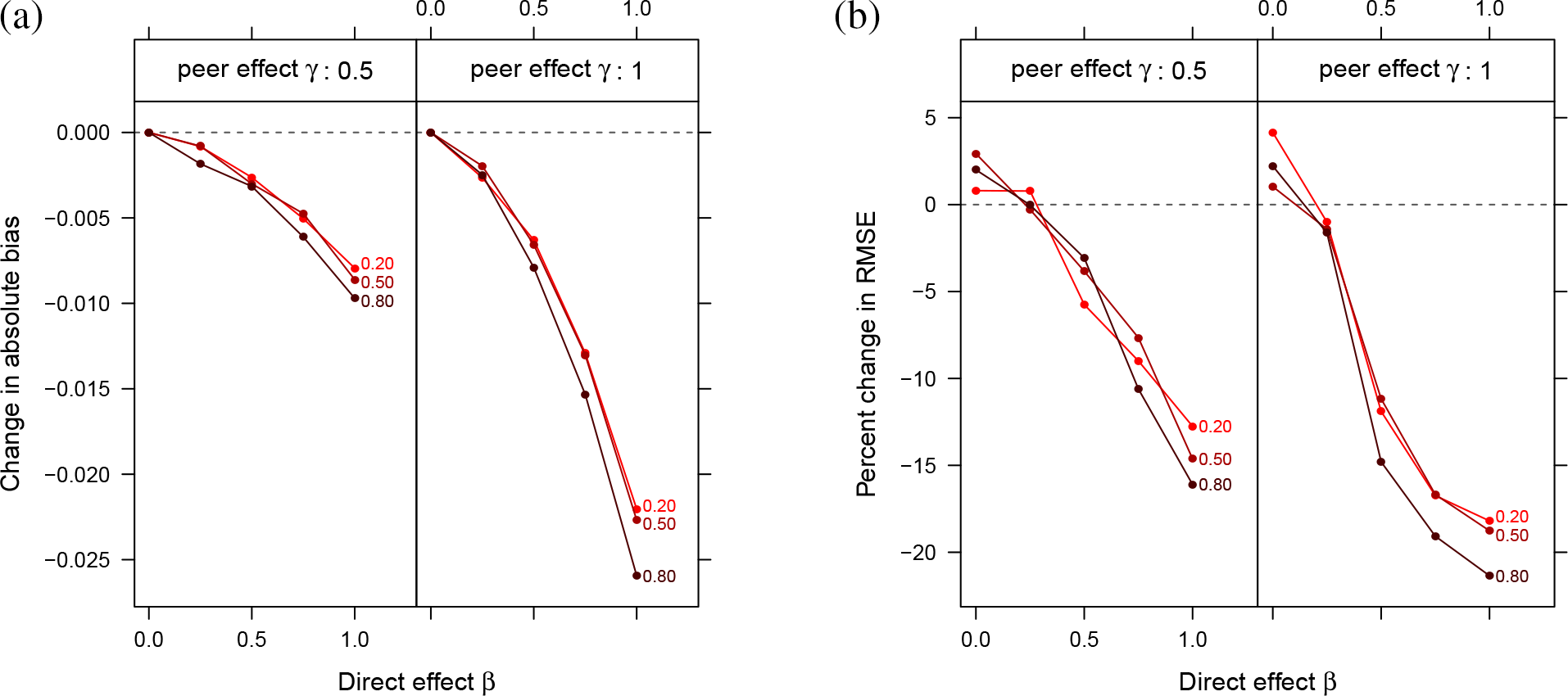
Change in (a) bias and (b) RMSE due to clustered random assignment. Lines are labeled with the expected proportion of edges that are within a community
Figure 8(a) displays bias as a function of both design and analysis decisions. As with the small-world networks, estimators making use of the
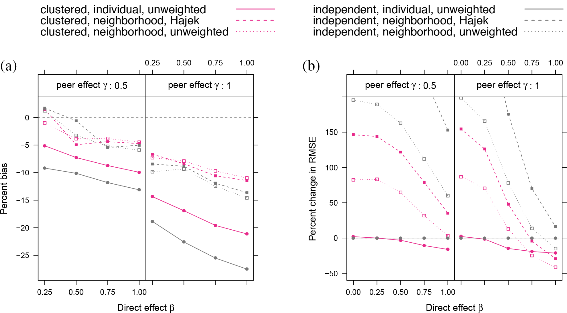
Relative bias (a) and change in RMSE (b) in ATE estimates for different assignment procedures, exposure models, and estimation method, using the degree-corrected block model with community proportion
4 Discussion
Recent work on estimating effects of global treatments in networks through experimentation has generally started with a particular set of assumptions about patterns of interference, such as the neighborhood treatment response (NTR) assumption, that make analysis tractable and then developed estimators with desirable properties (e.g., unbiasedness, consistency) under these assumptions [14, 15]. Similarly, Ugander et al. [16] analyzed graph cluster randomization under such assumptions. Unfortunately, these tractable exposure models are also made implausible by the very processes, such as peer effects or social interactions, that are expected to produce interference in the first place. Therefore, we have considered what can be done to reduce bias from interference when such restrictions on interference cannot be assumed to apply in reality.
The theoretical analysis in this paper offers sufficient conditions for this bias reduction through design and analysis in the presence of potentially global interference. To further evaluate how design and analysis decisions can reduce bias, we reported results from simulation studies in which outcomes are produced by a dynamic model that includes peer effects. These results suggest that when networks exhibit substantial clustering and there are both substantial direct and indirect (via peer effects) effects of a treatment, graph cluster randomization can substantially reduce bias with comparatively small increases in variance. Significant error reduction occurred with networks of only 1,000 vertices, highlighting the applicability of these results to experiments with networks of varied sizes – not just massive networks. Since a prior version of this paper, these bias and reduction results have been replicated on a subgraph of a large online social network [41]. Additional reductions in bias can be achieved through the specific estimators used, even though these estimators would usually be motivated by incorrect assumptions about effective treatments.
We have focused on improving estimates of effects of global treatments, but we have not addressed statistical inference that is robust to network dependence. Experimenters will generally want to conduct statistical inference, such as testing null hypotheses of no effects of the treatment or producing confidence intervals for estimated ATEs. Standard methods for randomization inference can be used to test the sharp null hypothesis that the treatment has no effects whatsoever (e.g., permutation tests for clustered randomization). Other hypotheses, such as those about the presence of spillover effects (i.e., SUTVA, the ITR assumption), can be tested exactly either by assuming constant direct effects [19] or using conditional randomization inference for non-sharp null hypotheses [18, 22].
Further work should examine how our results apply to other networks and data-generating processes. The main theoretical analysis and simulations in this paper used models in which outcomes are monotonic in treatment and peer behavior. Such models are a natural choice given many substantive theories; for example, when there are strategic complements in the behavior. On the other hand, non-monotonic responses are expected when having a mix of treated and control neighbors is more different from either having all treated or control neighbors (e.g., inconsistent service offerings to neighbors result in fewer purchases). Other cases where we expect non-monotonic responses include cases where value of engaging in a behavior is determined by a market (e.g., completing a job training program). Our simulations did not include vertex characteristics (besides degree) and prior behaviors, which could play an important role in the bias and variance for different designs and estimators.
Much of the empirical literature that considers peer effects in networks, whether field experiments, e.g. [42, 43, 45, 46], or observational studies, e.g. [36, 47], has aimed to estimate peer effects themselves, rather than estimating effects of interventions that work partially through peer effects. This may reflect differences in the quantities of interest for some topics in social science and for decision-making about potential interventions. It is important to note that the intuitions that motivate the clustered designs examined here may not apply to these other estimands (e.g., the case of trying to separately estimate direct and indirect effects). A fruitful direction for future work would involve directly modeling the peer effects involved and then using these models to estimate effects of global treatments, cf. [48].[23] This could substantially expand the range of designs and analysis methods to consider.
Acknowledgements
We are grateful for comments from Edoardo Airoldi, Eytan Bakshy, Thomas Barrios, Guido W. Imbens, Stephen E. Fienberg, Daniel Merl, Cyrus Samii, and participants in the Statistical and Machine Learning Approaches to Network Experimentation Workshop at Carnegie Mellon University and in seminars in the Stanford Graduate School of Business, Columbia University’s Department of Statistics, New York University’s Department of Politics, UC Davis’s Department of Statistics, and Johns Hopkins University’s Department of Biostatistics, and from anonymous referees. D.E. was an employee of Facebook while contributing to prior versions of this paper, remains a contractor with Facebook, and has a significant financial interest in Facebook.
Appendix
A Modified graph cluster randomization: Hole punching
We now briefly present a simple modification of graph cluster randomization that adds vertex-level randomness to the treatment assignment, such that some vertex assignments may not match their cluster assignment. We set
The
B Bias reduction from design: balanced linear case
In this appendix, we consider the linear outcome model under an alternative graph cluster randomization that enforces balance (i.e., equal sample sizes in treatment and control) Assume there is an even number of clusters
Theorem A.1
Assume we have a outcome model for all vertices
Then for some mapping of vertices to clusters
Proof.
Using the linear model for
for this outcome model. Under balanced graph cluster randomization,
We can extend this to the case where the mapping of vertices to clusters is random:
Separating out
If we have uniform probability over all cluster assignments with the same number of vertices per cluster, then for
so
Under balanced independent assignment, we just have
Because
which is the same expression as the relative bias for graph cluster randomization except for the multiplicative factor in the front. For large enough
C Bias reduction from analysis
Here we restate and prove Theorem 2.3 from the main text. We also consider two possible extensions of this theorem to graph cluster randomization (from independent random assignment), giving a counterexample for one extension and proving an analog of the theorem for the other extension.
Consider functions
Definition 2.2
If we have two such functions
Theorem 2.3
Let
Proof.
All expectations are taken with respect to independent random assignment. Assume monotonically increasing responses for every vertex and select an arbitrary vertex
This quantity is the expectation of the potential outcome for
To reduce the notation in what follows, we define
Due to independent random assignment, conditioning on
In this process,
Since the design is independent random assignment, we have that
where in the second equality we have used that
Since this inequality applies for all vertices
from which we immediately conclude that
The proof for monotonically decreasing responses follows when switching the inequalities throughout the above.
Consider some vertex
While this counterexample demonstrates that using more restrictive exposure conditions of this kind is not always helpful under graph cluster randomization, we do observe bias reduction in our simulations using graph cluster randomization without meeting the sufficient conditions of the theorem. In general, we expect that for bias to increase, there must be heterogeneous effects across heterogeneously sized clusters as in the counterexample above.
In fact, with a redefinition of the exposure conditions, we can provide a similar proposition that does include graph cluster randomization and also encompasses independent assignment as a special case.
Corollary A.2
Consider a fixed set of clusters which will be used for graph cluster randomization. Let function
Proof.
This proof is essentially the same as for Theorem 2.3 except
expectations are computed with respect to graph cluster randomization instead of independent treatment assignment, and references to 1’s and 0’s apply to clusters in
An important special case of this corollary covers the comparison of FNTR with ITR under graph cluster randomization, since FNTR and ITR can be written as cluster-level exposure conditions of this kind.
D Additional simulations with non-monotonic responses
The simulations reported in the main text, while not satisfying the conditions for graph cluster randomization to be bias reducing given by Theorem 2.1, did nonetheless have responses monotonically increasing with respect to
We repeat the simulations with small world networks in Section 3 with the following change. We run the process 1,000 times for all combinations of
Figure 9 shows the results of these simulations. Graph cluster randomization results in bias reduction, and for larger (in absolute terms) values of
Changes in bias and root-mean-squared-error (RMSE) due from clustered random assignment for small world networks with non-monotonic responses and prw = 0.01.
References
1. Manski CF. Economic analysis of social interactions. J Econ Perspect 2000;14:115–136.10.3386/w7580Suche in Google Scholar
2. Moffitt RA. Policy interventions, low-level equilibria, and social interactions. Durlauf SN, Young HP, editors. Social Dynamics. Cambridge, MA: MIT Press, 2001:45–82. .10.7551/mitpress/6294.003.0005Suche in Google Scholar
3. Bond RM, Fariss CJ, Jones JJ, Kramer AD, Marlow C, Settle JE, et al. et al. A 61-million-person experiment in social influence and political mobilization. Nature 2012;489:295–298.10.1038/nature11421Suche in Google Scholar PubMed PubMed Central
4. Bakshy E, Eckles D, Bernstein MS. Designing and deploying online field experiments. In Proceedings of the 23rd International Conference on World Wide Web, 2014:283–292.10.1145/2566486.2567967Suche in Google Scholar
5. Kohavi R, Longbotham R, Sommerfield D, Henne RM. Controlled experiments on the web: Survey and practical guide. Data Min Knowl Discovery 2009;18:140–181.10.1007/s10618-008-0114-1Suche in Google Scholar
6. Hudgens MG, Halloran ME. Toward causal inference with interference. J Am Stat Assoc 2008;103(482):832–842.10.1198/016214508000000292Suche in Google Scholar PubMed PubMed Central
7. Sobel ME. What do randomized studies of housing mobility demonstrate? Causal inference in the face of interference. J Am Stat Assoc 2006;101:1398–1407.10.1198/016214506000000636Suche in Google Scholar
8. Tchetgen EJ, VanderWeele TJ. On causal inference in the presence of interference. Stat Methods Med Res 2012;21:55–75.10.1177/0962280210386779Suche in Google Scholar PubMed PubMed Central
9. Toulis P, Edward K. Estimation of Causal Peer Influence Effects (Proceedings of The 30th International Conference on Machine Learning). J Mach Learn Res W&CP 2013. 28(3):1489–1497.Suche in Google Scholar
10. Baird S, Bohren JA, McIntosh C, Ozler B. (2014). Designing experiments to measure spillover effects. Policy Research Working Papers. Waschington, D.C., The World Bank.10.1596/1813-9450-6824Suche in Google Scholar
11. Holland PW. Causal inference, path analysis, and recursive structural equations models. Sociol Methodol 1988;18:449–484.10.2307/271055Suche in Google Scholar
12. Rubin DB. Estimating causal effects of treatments in randomized and nonrandomized studies. J Educ Psychol 1974;66:688–701.10.1037/h0037350Suche in Google Scholar
13. Cox DR. Planning of Experiments. Hoboken, New Jersey: Wiley, 1958 .Suche in Google Scholar
14. Manski CF. Identification of treatment response with social interactions. Econom J 2013;16. S1–S23.10.1920/wp.cem.2010.0110Suche in Google Scholar
15. Aronow P, Samii C. Estimating average causal effects under general interference (Working Paper). 2014; Available at http://arxiv.org/abs/1305.6156.Suche in Google Scholar
16. Ugander J, Karrer B, Backstrom L, Kleinberg JM. Graph cluster randomization: network exposure to multiple universes. Proceedings of the 19th ACM SIGKDD international conference on knowledge discovery and data mining (KDD ‘13). Dhillon IS, Koren Y, Ghani R, Senator P, Bradley J, Parekh R, et al., editors. New York: ACM, 2013:329–337.10.1145/2487575.2487695Suche in Google Scholar
17. Rosenbaum PR. Interference between units in randomized experiments. J Am Stat Assoc 2007;102.10.1198/016214506000001112Suche in Google Scholar
18. Aronow PM. A general method for detecting interference between units in randomized experiments. Sociol Methods Res 2012;41:3–16.10.1177/0049124112437535Suche in Google Scholar
19. Bowers J, Fredrickson MM, Panagopoulos C. Reasoning about interference between units: a general framework. Polit Anal 2013;21:97–124.10.1093/pan/mps038Suche in Google Scholar
20. Coppock A, Sircar N. An experimental approach to causal identification of spillover effects under general interference (Working Paper). 2013 Available at https://nsircar.files.wordpress.com/2013/02/coppocksircar_20130718.pdf.Suche in Google Scholar
21. Choi DS. (2014). Estimation of monotone treatment effects in network experiments. J Am Stat Assoc. doi:10.1080/01621459.2016.1194845.Suche in Google Scholar
22. Athey S, Eckles D, Imbens GW. Exact p-values for network interference. J Am Stat Assoc 2016 Available at http://arxiv.org/abs/1506.02084.10.3386/w21313Suche in Google Scholar
23. Walker D, Muchnik L. Design of randomized experiments in networks. Proc IEEE 2014;102:1940–1951.10.1109/JPROC.2014.2363674Suche in Google Scholar
24. Watts DJ, Strogatz SH. Collective dynamics of ‘small-world’ networks. Nature 1998;393:440–442.10.1515/9781400841356.301Suche in Google Scholar
25. Karrer B, Newman ME. Stochastic blockmodels and community structure in networks. Phys Rev E 2011;83:016107.10.1103/PhysRevE.83.016107Suche in Google Scholar PubMed
26. Fortunato S. Community detection in graphs. Phys Rep 2010;486:75–174.10.1016/j.physrep.2009.11.002Suche in Google Scholar
27. Newman ME. Modularity and community structure in networks. Proc Natl Acad Sci 2006;103:8577–8582.10.1073/pnas.0601602103Suche in Google Scholar PubMed PubMed Central
28. Fortunato S, Barthelemy M. Resolution limit in community detection. Proc Natl Acad Sci 2007;104:36–41.10.1073/pnas.0605965104Suche in Google Scholar PubMed PubMed Central
29. Pearl J. Causality: Models, Reasoning and Inference. Cambridge, UK: Cambridge University Press, 2009 .10.1017/CBO9780511803161Suche in Google Scholar
30. Young HP. Individual Strategy and Social Structure: An Evolutionary Theory of Institutions. Princeton, NJ, USA: Princeton University Press, 1998.10.1515/9780691214252Suche in Google Scholar
31. Blume LE. The statistical mechanics of best-response strategy revision. Game Econ Behav 1995;11:111–145.10.1006/game.1995.1046Suche in Google Scholar
32. Jackson MO. Social and Economic Networks. Princeton, NJ, USA: Princeton University Press, 2008.10.1515/9781400833993Suche in Google Scholar
33. Manski CF. Identification of endogenous social effects: The reflection problem. Rev Econ Stud 1993;60:531–542.10.2307/2298123Suche in Google Scholar
34. Lee LF. Identification and estimation of econometric models with group interactions, contextual factors and fixed effects. J Econom 2007;140:333–374.10.1016/j.jeconom.2006.07.001Suche in Google Scholar
35. Bramoulle Y, Djebbari H, Fortin B. Identification of peer effects through social networks. J Econom 2009;150:41–55.10.1016/j.jeconom.2008.12.021Suche in Google Scholar
36. Goldsmith-Pinkham P, Imbens GW. Social networks and the identification of peer effects. J Bus & Econ Stat 2013;31:253–264.10.1080/07350015.2013.801251Suche in Google Scholar
37. Middleton JA. Bias of the regression estimator for experiments using clustered random assignment. Stat Probab Lett 2008;78:2654–2659.10.1016/j.spl.2008.03.008Suche in Google Scholar
38. Middleton JA. and Aronow PM. Unbiased Estimation of the Average Treatment Effect in Cluster-Randomized Experiments. Statistics, Politics and Policy 2015; 6(1-2), pp.39-75.10.1515/spp-2013-0002Suche in Google Scholar
39. Ugander J, Karrer B, Backstrom L, Marlow C. (2011).The anatomy of the Facebook social graph (Technical report) Available at http://arxiv.org/abs/1111.4503Suche in Google Scholar
40. Blondel VD, Guillaume JL, Lambiotte R, Lefebvre E. Fast unfolding of communities in large networks. J Stat Mech Theor Exp 2008;2008:10008.10.1088/1742-5468/2008/10/P10008Suche in Google Scholar
41. Gui H, Xu Y, Bhasin A, Han J. Network A/B testing: from sampling to estimation. Proceedings of the 24th international conference on World Wide Web. New York: ACM, 2015;399–409.10.1145/2736277.2741081Suche in Google Scholar
42. Aral S, Walker D. Creating social contagion through viral product design: a randomized trial of peer influence in networks. Manage Sci 2011;57:1623–1639.10.1287/mnsc.1110.1421Suche in Google Scholar
43. Bakshy E, Eckles D, Yan R, Rosenn I. Social influence in social advertising: evidence from field experiments. Proceedings of the 13th ACM Conference on Electronic Commerce (EC ‘12). New York: ACM, 2012;146–161.10.1145/2229012.2229027Suche in Google Scholar
44. Bakshy E, Rosenn I, Marlow C, Adamic L. The role of social networks in information diffusion. Proceedings of the 21st international conference on World Wide Web (WWW ‘12). New York: ACM, 2012;519–528. DOI: 10.1145/2187836.2187907.Suche in Google Scholar
45. Bapna R, Umyarov A. Do your online friends make you pay? A randomized field experiment on peer influence in online social networks. Management Science 2015; 61(8), pp.1902-1920.10.1287/mnsc.2014.2081Suche in Google Scholar
46. Eckles D, Kizilcec RF, Bakshy E. Estimating peer effects in networks with peer encouragement designs. Proc Natl Acad Sci 2016;113:7316–7322.10.1073/pnas.1511201113Suche in Google Scholar PubMed PubMed Central
47. Aral S, Muchnik L, Sundararajan A. Distinguishing influence-based contagion from homophily-driven diffusion in dynamic networks. Proc Natl Acad Sci 2009;106:21544–21549.10.1073/pnas.0908800106Suche in Google Scholar PubMed PubMed Central
48. van der Laan MJ. Causal inference for a population of causally connected units. J Causal Inference 2014;2(1):1–62.10.1515/jci-2013-0002Suche in Google Scholar PubMed PubMed Central
© 2017 Walter de Gruyter GmbH, Berlin/Boston
This article is distributed under the terms of the Creative Commons Attribution Non-Commercial License, which permits unrestricted non-commercial use, distribution, and reproduction in any medium, provided the original work is properly cited.
Artikel in diesem Heft
- Research Articles
- Design and Analysis of Experiments in Networks: Reducing Bias from Interference
- Interventional Approach for Path-Specific Effects
- Entropy Balancing is Doubly Robust
- Semi-Parametric Estimation and Inference for the Mean Outcome of the Single Time-Point Intervention in a Causally Connected Population
- Identification of the Joint Effect of a Dynamic Treatment Intervention and a Stochastic Monitoring Intervention Under the No Direct Effect Assumption
- Causal, Casual and Curious
- A Linear “Microscope” for Interventions and Counterfactuals