Banking Crises Under a Central Bank Digital Currency (CBDC)
-
Lea Bitter


Abstract
One of the main concerns associated with central bank digital currencies (CBDC) is the disintermediating effect on the banking sector in general, and the risk of bank runs in times of crisis in particular. This paper examines the implications of an interest-bearing CBDC on banking crises in a dynamic bank run model with a financial accelerator. The analysis distinguishes between bank failures due to illiquidity and due to insolvency. In a numerical exercise, CBDC leads to a reduction in the net worth of banks in normal times but mitigates the risk of a bank run in times of crisis. The financial stability implications also depend on how CBDC is accounted for on the asset side of the central bank balance sheet: if CBDC issuance is complemented by asset purchases, it delays the onset of both types of bank failures to larger shocks. In contrast, if CBDC issuance is complemented by loans to banks, it substantially impedes failures due to illiquidity, but only marginally affects bank failures due to insolvency.
1 Introduction
Digital transformation has and will further change our payment and monetary system. Throughout history, money has adapted over time and its form has changed significantly – from cowrie shells and commodity money to commodity-backed money and fiat money. To adjust to the developments of an increasingly digital payment system, central banks have started to explore the potential of a central bank digital currency (CBDC).[1] A retail CBDC would be inherently risk-free public money, similar to cash, but with the additional convenience of being digital and entailing the option to bear interest. These features make CBDC a closer substitute to bank deposits which could adversely affect the deposit funding of commercial banks.
One of the main concerns in the discussion on CBDC revolves around its impact on the banking sector in general, but especially in times of crisis (e.g. see, Bank for International Settlements 2018; Carney 2018; ECB 2020). The general fear is that an attractive CBDC could structurally disintermediate the banking sector. These fears are amplified in times of crisis. Both deposits and CBDC are digital, convenient, and potentially interest-bearing, making them relatively close substitutes. This relatively close substitutability of deposits and CBDC, combined with the inherently riskless nature of public money, raises the concern that a CBDC may trigger bank runs more easily. When confidence in the financial system is low, a CBDC may provide an attractive outside option, thereby reducing the cost to depositors of withdrawing their funds from the bank. The potentially lower cost to depositors of participating in a bank run raises concerns that runs may occur under a CBDC when depositors otherwise would not have run. A further concern is that runs could unfold more quickly due to the (potentially unlimited) 24/7 digital access to CBDC.
This paper shows that the concerns outlined in the previous paragraph may not necessarily substantiate. Analysing these concerns in a dynamic bank-run framework, I find that a CBDC does indeed make bank runs less disruptive, but this does not impair financial stability; on the contrary, it makes it more difficult for bank runs to occur. The results highlight the significance of assessing the general equilibrium effects of the introduction of a CBDC on financial stability. Particularly, the asset-side adjustments on the central bank’s balance sheet resulting from CBDC issuance can have a stabilising impact on the economy that can dominate the disintermediating impact of the outflow of deposits into CBDC.
To study the impact of a CBDC on aggregate banking crises and the possibility of systemic bank runs, I introduce an interest-bearing CBDC into the dynamic bank run framework of Gertler and Kiyotaki (2015).[2] The framework allows to combine financial accelerator dynamics with the emergence of bank runs, which are based on macroeconomic fundamentals but ultimately triggered by beliefs. Such framework also allows to distinguish between bank failures due to illiquidity and insolvency. In contrast to alternative bank run frameworks in the literature, which are mostly limited to two or three periods, in the Gertler and Kiyotaki (2015) framework households and banks optimise in an infinite horizon economy, allowing for richer and more realistic dynamics.
The stylised endowment economy with financial frictions consists of households, banks, and a central bank which issues CBDC following an interest-rate rule. Serving as proxy for the firm sector, capital is modelled as a productive technology yielding a return each period that is subject to aggregate shocks. Households can place their savings in CBDC, bank deposits, or capital. The model analysis abstracts from cash and focuses only on deposit substitution into CBDC which is the more relevant case and a more conservative assumption for financial stability considerations.
The analysis allows to distinguish between banking failures due to illiquidity and bank failures due to insolvency. While banks are most efficient in intermediating capital, they are limited by a leverage constraint. In normal times, the model features a unique equilibrium in which banks intermediate the majority of assets. However, if a sufficiently large shock hits the economy, a second equilibrium emerges which is characterised by a bank run on the entire banking system. Bank failures due to illiquidity can emerge if households withdraw their deposits because they believe that other agents will run, leading to a bank run triggered by self-fulfilling beliefs. If the shocks become even larger, at a certain point only the bank run equilibrium remains and banks fail due to insolvency.
The introduction of a CBDC creates an additional liability on the central bank balance sheet that will lead to further balance sheet adjustments, contributing to the impact of a CBDC on the economy. This paper accounts for the potentially varying implications of different balance sheet adjustments by analysing CBDC issuance in the context of two policy scenarios: in the first policy scenario, the central bank complements CBDC issuance on the liability side by lending to banks on the asset side of the central bank’s balance sheet (‘credit policy’); in the second policy scenario, the central bank complements CBDC issuance by purchasing capital securities (‘asset policy’). Both policy scenarios would lead to an increase in the central bank balance sheet and are contrasted to the economy without a CBDC (‘no CBDC’).[3]
A simulation of the model offers four main insights: first, in steady state, a CBDC does not majorly affect aggregate output and prices but it does affect the composition of household savings, bank funding and capital investment, leading to a reduction in bank profits. Second, both CBDC policy scenarios tend to have a small but stabilising influence in a crisis that does not trigger a bank run. Third, these stabilising effects become more important in a bank run situation: both CBDC policy scenarios improve financial stability by postponing the emergence of bank runs to larger shocks. Fourth, the impact of a CBDC also depends on the accompanying central bank balance sheet adjustments; CBDC issuance with ‘asset policy’ delays the onset of both types of bank failures to larger shocks. In contrast, CBDC issuance with ‘credit policy’ substantially impedes failures due to illiquidity, but has little impact bank failures due to insolvency.[4] Overall, while CBDC issuance strains the banking sector in steady state by reducing deposits and net worth, it improves financial stability in times of crisis by impeding the emergence of bank runs.
What mechanism lies at the root of the result that CBDC issuance delays the emergence of bank runs – a result that runs contrary to the initially stated concerns? In the model framework, CBDC issuance makes bank runs less disruptive because the central bank channels CBDC inflows back into the economy, either via credit to banks or direct capital purchases. This reduces the burden on households and increases the efficiency and price of capital. These central bank interventions that channel the CBDC inflows back into the economy slow the financial accelerator dynamics and make the occurrence of bank runs more difficult, ultimately postponing their occurrence to larger shocks.
Naturally, the central bank can take measures independent of CBDC issuance to improve financial stability and to avert systemic runs. The main insight of this model analysis is that in a bank run situation inflows into CBDC, instead of inflows into other less efficient assets, are aligned with financial stability measures and do not exacerbate bank run risks. In a bank run situation, households do not withdraw deposits because they like CBDC but because they are concerned about the safety of their deposits. By providing them with a safe and more efficient alternative to run into, the issuance of CBDC mitigates losses in a bank run scenario, stabilising capital prices and making runs less likely from the outset.
Context of the literature: The related literature also supports a nuanced picture of the financial stability implications of a CBDC. The issuance of CBDC is found to have ambiguous financial stability implications, depending not only on adjustments on the asset side of the central bank’s balance sheet but also on information effects, the structure of the financial sector, CBDC remuneration, and other notable design parameters.[5]
Overall, the results of Keister and Monnet (2022) and Muñoz and Soons (2024) are qualitatively in line with the insights of this paper, finding a benign impact of CBDC on financial stability. Both Keister and Monnet (2022) and Muñoz and Soons (2024) find that under a CBDC banks have the incentive to rebalance their portfolio more towards long-term liabilities and lending which reduces the maturity mismatch of bank assets and tends to improve financial stability. Consistent with the mechanism included in this paper, in the model of Keister and Monnet (2022) the anticipation of a less severe bank run scenario reduces the incentive to run from the outset. Furthermore, Keister and Monnet (2022) argue that the issuance of CBDC gives the central bank an information advantage on financial stability conditions through which it can intervene more efficiently.[6]
In the papers of Kim and Kwon (2023), Ahnert et al. (2023), Lucas (2022), and Skeie (2021), the directional financial stability implications of a CBDC are context-dependent. The importance of the asset side counterpart to CBDC operations is similarly highlighted by Kim and Kwon (2023) in an OLG model with a different definition of bank runs. In their model, bank runs are not self-fulfilling but set up as situations in which depositors who need to withdraw money cannot be fully repaid. They find that CBDC issuance that is complemented by loans to banks increases financial stability. However, when the complementing asset side operations are neither directly (e.g. via direct lending) or indirectly (e.g. via stabilising asset prices via asset purchases) supporting banks, then the issuance of a CBDC deteriorates financial stability.
In Ahnert et al. (2023), Lucas (2022), and Skeie (2021), the remuneration policy of CBDC and central bank refinancing operations is key to determine the impact on financial stability. In the global game analysis of the two-period bank run model of Ahnert et al. (2023), CBDC remuneration has two countervailing forces that can either increase or decrease financial fragility and the probability of a bank run. While a higher CBDC remuneration increases the incentive for deposit withdrawal, it also induces banks to offer more attractive deposit conditions, reducing the incentive to withdraw deposits. The overall impact is ultimately determined by the responsiveness of deposit conditions to CBDC remuneration which depends on the degree of market power. Lucas (2022) shows that the central bank can prevent bank runs by allowing central bank refinancing operations at sufficiently attractive conditions for banks. Similarly, Skeie (2021) finds that bank runs into CBDC can be prevented by dynamically adjusting remuneration of CBDC and reserves. The significance of remuneration as a design parameter is also reflected in this paper, in which the dynamic adjustment of CBDC issuance conditions in response to fluctuations in CBDC demand and output plays an important role in the overall impact.
The result that CBDC issuance makes banking panics less disruptive is also is in line with the findings of Williamson (2021). However, in contrast to Keister and Monnet (2022) and this paper, the lesser severity of runs tends to encourage banking panics. This opposite finding in the model of Williamson (2021) can be explained by CBDC offering an improved alternative to retail payments and thereby replacing payments that would otherwise have been made with deposits. Therefore, in their model the ability of CBDC to ensure payment efficiency during a run, reduces the cost of running and in this case makes runs more likely.
There are several papers studying the structural impact of CBDC on financial intermediation, complementing the analyses of the impact of CBDC during a financial crisis (e.g. see Andolfatto 2021; Chiu et al. 2023; Keister and Sanches 2023). Ahnert et al. (2022) and Chapman et al. (2023) both survey the growing CBDC literature with a specific focus on financial intermediation and stability. Several papers discuss policy measures aimed to prevent excessive CBDC holdings, such as holding limits (Assenmacher et al. 2021; Bindseil, Panetta, and Terol 2021; Meller and Soons 2023), tiered remuneration (Bindseil 2019), and limited convertibility with reserves and deposits (Kumhof and Noone 2021).
This paper contributes to the literature on financial stability implications of a CBDC in three ways. First, it focuses explicitly on the potentially varying implications of different central bank balance sheet asset side adjustments in response to CBDC issuance. Second, it distinguishes between banking failures due to illiquidity and insolvency and assessing the implications of a CBDC on the realisation of both types of banking failures. Third, while the above papers mostly analyse financial stability implication in a two or three period model, this paper analyses the financial stability implications in a more dynamic infinite horizon economy with a financial accelerator. The presented model focuses on the store of value function of money as it is most important in the context of bank runs. However, the analysis neglects the role of money as a medium of exchange even though most central banks aim to design CBDC as a means of exchange rather than an attractive store of value. Furthermore, the model poses a very stylised real setting which could be extended to an economy with a richer firm sector, nominal frictions, conventional monetary policy, and a more sophisticated government sector.
Hereinafter, Section 2 discusses central bank balance sheet adjustments to CBDC issuance in more detail. Section 3 presents the general model economy and the bank run scenarios which is subsequently simulated and analysed in Section 4. Finally, Section 5 concludes.
2 CBDC Issuance and the Central Bank Balance Sheet
This section reviews different scenarios of how CBDC issuance can affect the central bank balance sheet. The analysis highlights the relevance of taking into account central bank balance sheet adjustments in response to CBDC issuance for equilibrium dynamics and provides motivation for the two scenarios employed in the subsequent model analysis.
2.1 General Central Bank Balance Sheet Dynamics of CBDC Issuance
The idea of opening the central bank balance sheet to deposits by the public is not new. Quite contrary, it was a common central bank practice until mid-20th century. As e.g. elaborated by Fernández-Villaverde et al. (2021), historically many major central banks not only allowed deposits but also granted loans to private firms and individuals. The idea of enabling deposits at the central bank for the public was prominently brought back on stage and into the electronic sphere by Tobin (1985, 1987) from which the current discussion mostly picks up.
The introduction of a CBDC would create a new type of liability that can trigger different adjustments on the central bank balance sheet, contributing in different ways to determine the equilibrium impact of a CBDC. For instance, Barker, Bholat, and Thomas (2017) argue that “although there has been a lot of discussion about how central bank digital currency could radically change payment systems – and even the financial sector as a whole – the implication for the assets on central bank balance sheets could be just as critical”. However, in most CBDC model analyses, the modelling choice that complements CBDC issuance on the central bank balance sheet remains in the background and its implications are not explicitly discussed.[7] In practice, these balance sheet adjustments will depend on monetary policy, the economic and institutional context and will be difficult to link directly to CBDC. Nonetheless, for analytical purposes, evaluating the impact of different measures in isolation can provide valuable insights.
This paper focuses on the most relevant CBDC scenarios which would lead to an increase in the central bank balance sheet. CBDC issuance will either lead to rearrangements on the liability side of the central bank balance sheet or to an increase in both, liabilities and assets. In most cases, either cash or deposits will be substituted into CBDC.[8] The substitution of cash into CBDC would simply constitute a change in the type of central bank money held by the public and would be neutral from a financial stability perspective.[9] Therefore, the following analysis abstracts from cash and focuses only on deposit substitution into CBDC. The substitution of deposits into CBDC would either lead to a reduction in excess reserves (no impact on the size of the central bank balance sheet) or require a counterposition on the asset side (increasing the size of the central bank balance sheet).[10] Situations in which deposit outflows cannot be absorbed by a reduction in excess reserves pose more serious financial stability concerns. Therefore, for simplicity the following analysis abstracts from modelling reserves and focuses on scenarios in which CBDC issuance leads to an increase in the central bank balance sheet.
2.2 Deposit Substitution into CBDC via Central Bank Credit (‘Credit Policy’)
As a first and most prominently discussed option, the central bank could increase its credit operations to banks in order to complement CBDC issuance. Such adjustments would channel lost deposit funding back to the banks in the form of central bank credit. Lending to financial institutions is already a substantial component of central bank assets in normal times but becomes particularly important in times of crisis. The role of the central bank as ‘lender of last resort’, dating back to Bagehot (1873), is also documented by Pattipeilohy (2016) who shows a clear shift towards private sector lending (including banks) by the Federal Reserve, Bank of England and the Eurosystem in response to the financial crisis from 2007 and onward.
Given the particular relevance of bank lending in times of crisis, the following model framework will explicitly review CBDC issuance with ‘credit policy’ as illustrated in Table 1.[11] This scenario also provides the basis for the ‘equivalence result of public and private money’ of Brunnermeier and Niepelt (2019) who show that equilibrium allocations stay unaltered under the assumption that CBDC is fully redistributed as credit to private banks (under the same conditions). Moreover, CBDC issuance with ‘credit policy’ is employed for instance also in the model analyses of Skeie (2021) and Kim and Kwon (2023).
CBDC issuance with credit policy in the stylised model framework.
| Households | Banks | Central bank | |||
|---|---|---|---|---|---|
| A | L | A | L | A | L |
| Capital Sec. | Equity | Capital Sec. | Deposits | Loans | CBDC |
| Deposits | (Endowment) | Loans | |||
| CBDC | Equity | ||||
2.3 Deposit Substitution into CBDC via the Sale of Assets (Asset Policy)
As a second option, the central bank could accept non-bank assets as a counterposition to CBDC issuance. Within the model framework, such a policy scenario would imply that deposits substituted into CBDC will not be replaced with central bank funding, leading to an immediate reduction in the private bank’s asset-side operations by the same amount. The assets exchanged in return for CBDC issuance would depend on what asset types would be accepted by the central bank and the assets available to banks. Within the stylised model framework of this paper, the ‘asset policy’ scenario would translate into purchases of capital securities by the central bank, visualised in Table 2, as banks only hold capital securities as asset. In practice, this scenario would be equivalent to central bank purchases of corporate bonds. Although still an unconventional monetary policy tool, corporate bond purchases have gained importance since the financial crisis and for instance have been applied to mitigate the impact of the coronavirus pandemic (e.g. see Cavallino et al. 2020). In the literature, CBDC issuance against corporate bonds has been modelled indirectly by Fernández-Villaverde et al. (2021) and directly by Schilling, Fernández-Villaverde, and Uhlig (2024), building on the seminal paper of Diamond and Dybvig (1983) in which the central bank invests into long-term projects (through an investment bank).
CBDC issuance with asset purchases in the stylised model framework.
| Households | Banks | Central bank | |||
|---|---|---|---|---|---|
| A | L | A | L | A | L |
| Capital Sec. | Equity | Capital Sec. | Deposits | Capital Sec. | CBDC |
| Deposits | (Endowment) | Equity | |||
| CBDC | |||||
In practice, government bonds will also be a prominent assets class to be accepted for CBDC issuance under the ‘asset policy’ scenario. Government bonds represent the largest asset share in the balance sheet of many central banks. This feature is vividly illustrated by Pattipeilohy (2016) who developed a classification scheme of central banks by their balance sheet composition, in which ‘Treasury holder’ is one important type. According to their analysis, most of the major central banks fell into this category in 2015. In the literature, CBDC issuance against government bonds has been modelled by Kim and Kwon (2023), Barrdear and Kumhof (2022), and Kumhof and Noone (2021) who even argue that CBDC should only be issued against government bonds.
Both types of asset policy options, CBDC issuance against government bonds and corporate bonds would lead to a reduction in private banks’ balance sheets. However, the second round and equilibrium effects will likely differ and depend on the presence of friction in the (model) economy. Within the model framework, central bank purchases of capital securities affect the valuation of capital and thus the financial accelerator. The implications of government bond purchases would depend on monetary-fiscal interactions (such as government debt dynamics), the modelling of the government sector (such as the fiscal regime) and the incentives for banks to hold government debt.[12] The model framework abstracts from these considerations on monetary-fiscal interactions and abstains from explicitly modelling the government sector to remain focused on financial stability considerations.[13]
3 Model Environment
This section introduces the above outlined two CBDC scenarios into the dynamic bank run framework of Gertler and Kiyotaki (2015), henceforth GK15. Following the GK15 model provides a ‘no CBDC’ benchmark which allows a comparison of the results under a CBDC with the results of GK15 without a CBDC. Section 3.1 outlines the stylised endowment economy with households, bankers, a central and capital as productive technology. Section 3.2 describes the emergence of banking failures due to self-fulfilling bank runs and due to insolvency.
3.1 General Model Framework
There are two types of goods in the economy: a non-durable consumption good C t and a durable capital good K t . The durable capital good acts as a stylised proxy for the firm sector, is of fixed supply, normalised to unity, and does not depreciate. A unit of capital at time t, K t , yields Zt+1 units of consumption in the next period and can be sold at the price Q t . The productivity of capital Z t is subject to a multiplicative aggregate shock and described by
where Z is aggregate productivity in steady state and ϵ z with E (ϵ z ) = 0 is a shock to productivity.
As in GK15, there are households and bankers in the economy, each with a unit mass of one. Households consume the nondurable consumption good and save. In addition to (i) investing directly in capital and (ii) holding bank deposits, I include as third option the possibility that households can (iii) hold CBDC. Banks are more efficient in managing capital but are subject to a leverage constraint. They maximise profits by investing funds from households and the central bank (under CBDC with ‘credit policy’) into capital. Furthermore, I introduce a central bank into the model that issues CBDC to households and complements funds on the asset side either via ‘credit policy’ by granting loans to banks or via ‘asset policy’ by investing into capital securities.
3.1.1 Households
The stylised model abstracts from labour choices and households receive an endowment of Z t W h units of the consumption good each period that is also subject to the productivity shock Z t . Households maximise lifetime utility
through the choice of consumption C t and saving for which they have three options:
Holding deposits D t which promise to pay a (non-contingent) gross rate of return
Directly investing in productive capital
Holding CBDC M t which pays the gross rate of
Furthermore, households receive a transfer T t from the central bank, paying out its seigniorage. If the central bank incurs losses (T t < 0) the transfer turns into lump-sum taxation. The household budget constraint is thus given by:
Maximising expected utility subject to the budget constraint yields the optimality conditions specifying that the return of all three assets must be equal to the inverse of the stochastic discount factor
3.1.2 Bankers
Environment: There is a unit mass of risk-neutral bankers, running their own financial intermediary. Bankers have a finite expected lifetime and in each period, there is an i.i.d. probability of 0 < 1 − σ < 1 that the banker will stop its activity and exits. Bankers enjoy consumption only upon exit by consuming their accumulated net worth. In each period, the same amount of 1 − σ new bankers enter with a starting capital of w
b
, such that the number of banks remains constant.[14] While in business, bankers aim to maximise their net worth n
t
by taking deposits from households d
t
at financing costs
The difference between the earnings from capital and the cost of deposits and central bank loans yields the net worth of the bank n t :
The franchise value V
t
of the bank is then the sum of the discounted probability of exiting in period i and consuming the accumulated net worth
In the absence of financial frictions, it would be optimal for all funds to be intermediated by the bank. However, bankers face an endogenous leverage constraint microfounded by a moral hazard problem: bankers can divert a certain fraction 0 < θ < 1 of assets for personal use. When deciding whether to ‘cheat’ or operate honestly, bankers compare the values of both options. With this knowledge, depositors and the central bank will only fund the bank to the extent that there is no incentive to divert funds. This leads to the constraint that the franchise value of the bank must always be greater than or equal to the gains from diverting assets which endogenously limits the debt to equity ratio of a bank.[16] However, it is assumed that the central bank is to a relatively lesser extent subject to the moral hazard risk. Due to its supervisory power and additional measures such as collateral requirements, the central bank is better at enforcing repayment from bankers, similarly modelled in Gertler and Kiyotaki (2010), Gertler and Karadi (2013), and Gertler, Kiyotaki, and Prestipino (2016b). Thus, for each unit of central bank credit supplied, a borrowing bank can only divert θ (1 − ω) with 0 < ω < 1. Accordingly, the moral hazard problem can be condensed into following incentive constraint:
General optimisation: The banker chooses
where
3.1.3 Central Bank
The representation of the central bank focuses on issuing an interest bearing CBDC. The model framework is only expressed in real terms and does not include inflation, and therefore the model also abstracts from conventional monetary policy.[18] In addition, the model abstracts from money as medium of exchange, focusing on the role of money as store of value which is central for studying financial stability and bank run aspects.
CBDC issuance: The central bank issues CBDC following an interest rate rule, but which can be expressed equivalently in terms of a quantity rule.[19]
Following this rule, the CBDC interest rate
While the issuance of CBDC on the liability side of the central bank balance sheet is the same for both analysed policy scenarios, the asset side setup differs under CBDC issuance with ‘credit policy’ and ‘asset policy’.
Credit Policy: The rule allocating credit to the banks under CBDC with ‘credit policy’ is straightforward. By assumption, this policy option complements CBDC issuance M t by providing credit to banks L t and thus all CBDC funds are channeled back to the banks:
The central bank redirects lost deposit funding exchanged in CBC back into the banking sector on a 1:1 basis and grants loans L
t
to banks equivalent to the amount of CBDC. The interest rate on central bank credit
The flow of central bank funds is then given by
where in each period the central bank issues CBDC M t and receives the loan repayments plus interest from the previous period. It uses the funds to repay the claims and interest on CBDC from the previous period and additionally grants new loans. The remainder is distributed as transfers T t to the households (or as tax in the case of a negative residue). In the absence of a bank run, the interest rate on loans is higher than the interest rate on CBDC; therefore, the transfers are positive despite being small.
Asset Policy: In contrast, under ‘asset policy’, the central bank does not accommodate CBDC with credit but buys capital securities itself. When investing into capital securities
The flow of funds of the central bank evolves similarly to Equation (11): the funds from CBDC and last period’s capital security returns are used to repay the claims of the CBDC from the previous period and for investments into new capital, plus management costs:
3.1.4 Aggregation, Timing and Equilibrium
Summarising the individual bank measures (denoted in lowercase letters) leads to the banking sector aggregate (denoted in capital letters). As there are a constant number of symmetric banks normalised to one and an equal amount of banks exit enter each period, aggregate net worth N t is a combination of the net worth of banks in operation and the endowment Wt b of newly entering banks:
Capital is of fixed supply and normalised to unity, therefore capital holding of households
Under CBDC with ‘asset policy’
Gross output, amounting to the sum of capital output Z
t
, household endowment Z
t
W
h
and bank endowment W
b
, is either consumed by households
However, output is defined without management costs i.e.
The sequence of events is as follows: at the beginning of period t, the productivity of capital Z t is realised. The new allocation of deposits, CBDC, loans, and capital investments are then determined. Deposits and loans are issued in a way that the moral hazard constraint is satisfied and the banker does not have the incentive to divert assets. The next period begins with the realisation of return on the capital invested the previous period.
Under CBDC with ‘credit policy’, the equilibrium is given by the vector of real prices
3.2 Bank Failures in the Model Environment
The equilibrium outlined above is based on the mutual beliefs of households about the deposit decisions of other households, in particular that they will not participate in a bank run. Under certain conditions, a second equilibrium among the above outlined ‘banking equilibrium’ exists, in which the belief of a bank run triggers a bank run in equilibrium (‘bank run equilibrium’). The following section examines the conditions under which a bank run equilibrium exists and how it unfolds under the different CBDC policy scenarios. The analysis considers only systemic bank runs, where banks are identical and subject only to aggregate shocks. In addition, the productivity shock to the economy that opens up the possibility of a bank run is unanticipated and therefore bank runs are also unanticipated.[21]
3.2.1 Types of Bank Failures
3.2.1.1 Bank Failures Due to Illiquidity
In each period, households decide whether to roll over their deposits to the next period. The individual decision to roll over deposits critically depends on the expectations of other households. If a household expects that other households will not roll over deposits and if this would leave the bank with zero assets, then it is individually rational not to roll over deposits as well. In such cases of a systemic bank, all households withdraw their deposits and banks are forced to liquidate their assets at the fire-sale price
on their claims
A bank run equilibrium exists if the haircut value becomes less than 1 (x t < 1). Conversely, if x t ≥ 1, all funds can be paid out in full and there is no reason to run, even if all other households run. Thus, the existence of a bank run equilibrium is determined by economic fundamentals, with the fire-sale value of the assets determining the haircut rate x t . Whether a bank run is triggered ultimately depends on the beliefs of households, with the bank run being induced in the model via a sunspot shock. If a bank run results in a default, the strategic complementarity in behaviour makes the belief of a bank run a self-fulfilling prediction. Self-fulfilling bank runs can be considered as bank failures due to illiquidity and are possible if:
3.2.1.2 Bank Failures Due to Insolvency
If a sufficiently large shock hits the economy and the bank’s liabilities exceed the value of its capital even at the non-fire-sale price Q t , it is rational for households to withdraw their deposits – regardless of the beliefs of other households. These bank runs driven by economic fundamentals can be considered as bank failures due to insolvency and are possible if:
The sole difference between the illiquidity and insolvency conditions in the ‘no CBDC’ scenario and the ‘asset policy’ CBDC scenario is the pricing of capital. There is a further difference in the ‘credit policy’ CBDC scenario: In the case of bank failures due to illiquidity, it is assumed that only households but not the central bank participate in the bank run. Instead, the central bank continues to lend to banks (see a more detailed description below). In contrast, in the case of bank failures due to insolvency, the central bank also withdraws its funding support and banks fail when the asset valuation cannot cover the full liabilities (i.e. deposits and central bank loans). Hence, the condition for a bank failure due to insolvency is met when the fundamental valuation of assets is less than the total liabilities (deposits and credit). In contrast, the condition for a bank failure due to illiquidity is met when the fire-sale valuation of assets is less than the value of deposits, i.e. only a subset of the total liabilities.
3.2.1.3 Equilibrium Ranges
The above scenarios lead to three possible equilibrium regions: in the first region, there is a unique equilibrium with functioning financial intermediation (‘banking equilibrium’). In the second region, the banking equilibrium and the bank run equilibrium coexist. Lastly, in the third region, only the bank run equilibrium remains. Based on the above conditions for the two types of bank failures, Table 3 shows the thresholds for the different equilibrium ranges, conditional on the evolution of capital productivity Z t .
Equilibrium ranges based on capital productivity Z t .
| Equilibria | Type of bank failures | CBDC asset policy & no CBDC | CBDC credit policy |
|---|---|---|---|
| Banking | None |
|
|
| Banking + bank run | Illiquidity |
|
|
| Bank run | Insolvency |
|
|
3.2.2 Bank Runs in the Different Policy Scenarios
How does a bank run unfold?[23] As a reference point, it is useful to first review the baseline scenario without a CBDC: a large shock is realised, triggering a bank run and households have no other option but to invest in capital themselves. However, households are only willing to purchase capital at a lower price due to their increasing marginal costs of managing capital: the higher costs of managing capital lead a fire-sale price of capital that is much lower than the non-bank-run price of capital. Although socially detrimental, individually it is still optimal to run and receive a haircut on deposit claims rather than losing the full deposit value.
In the ‘asset policy’ CBDC scenario, bank runs unfold in a similar way: households withdraw all deposits from the bank, the bank fails and closes down. The main difference here is that households can hold CBDC as a second asset. The relative return to households between holding capital and CBDC, determines the share that flows into CBDC and into capital. In this case, households but also the central bank invest into capital in the period of the bank run.
In the ‘credit policy’ CBDC scenario, bank runs remain similar for households but unfold differently for banks. As long as the bank is merely illiquid but not insolvent (see the conditions outlined above), only households participate in the run and withdraw their deposits while the central bank continues to grant credit. Households withdraw their deposits with a haircut, leaving the bank with no assets but outstanding debt to the central bank. In the period of the run, the bank defaults on its claims on the central bank. Without an intervention, the bank would go bankrupt. Instead, the central bank, in its spirit as ‘lender of last resort’, continues to lend to the bank in the amount of its CBDC inflows which enables the bank to continue to operate.[24] In the period of the bank run, the bank invests into capital only with central bank credit as it has zero net worth and zero deposits. Due to the outstanding claims of banks to the central bank, the capital return in the period of the run is fully paid out to the central bank. Ultimately, these measures prevent bank failures but also leave banks with zero net worth in the period after the run.
The central bank usually makes profit as the interest rate on credit is larger than the rate on CBDC. However, in the period of the bank run, the central bank absorbs the loss on the defaulted loans and the losses are distributed to households via lump-sum taxes (the transfers become negative). Nevertheless, in the period after the bank run, the central bank recovers some losses as it collects the full profit on invested capital by the bank and redistributes it to households.[25] In the period after the bank run, the banking sector starts to recover. Thus, in the ‘credit policy’ scenario, banks do not fail and their ability to intermediate capital efficiently can be maintained in the period of the bank run. At the same time, banks still start the period after the bank run with zero net worth and therefore are in the same situation as in the scenarios with ‘no CBDC‘ and CBDC with ‘asset policy’: with zero net worth it is as if these banks had failed and the sector must recover via newly entering banks.
4 Model Analysis
This section examines the dynamics of the economy under three different scenarios: CBDC with ‘credit policy’, CBDC with ‘asset policy’, and ‘no CBDC’. After explaining the calibration of the numerical exercise in Section 4.1, Section 4.2 analyses the implications of these three model scenarios in steady state. Subsequently, Section 4.3 examines the response of the economy to capital productivity shocks that do not lead to bank failures, whereas Section 4.4 focuses on bank failures and analyses the impact of the different CBDC policy scenarios. Specifically, the latter section investigates the required shock sizes after which self-fulfilling bank runs become possible (Section 4.4.1) and the shock sizes that lead to insolvency (Section 4.4.2). The aim of the analysis in this stylised endowment economy setup is not to aim for precisely matching empirical properties but rather to investigate the mechanisms influencing financial stability through the issuance of CBDC in the differing policy scenarios outlined above.
4.1 Calibration and Simulation
Table 4 lists all the parameter choices. Most of the parameters present in the ‘no CBDC’ scenario are taken from GK15, with the exception of the share of divertable assets θ = 0.22, which is updated to the value of Gertler, Kiyotaki, and Prestipino (2020). The introduction of a CBDC introduces additional parameters. Under CBDC issuance with ‘credit policy’, central bank credit to banks is, similar to deposit funding, also subject to a moral hazard constraint but only to half the extent and thus ω is set to 0.5 (e.g. as in Gertler and Karadi 2013). Similarly, under CBDC issuance with ‘asset policy’, the management cost of capital purchases α cb that the central bank faces is set to half the efficiency costs that households face.
Calibration of parameter values.
| Parameter | Value | Source | Description |
|---|---|---|---|
| α | 0.008 | GK15 | Marginal management costs households |
| α cb | 0.004 | New | Marginal management costs central bank |
| β | 0.99 | GK15 | Discount rate |
| σ | 0.95 | GK15 | Bankers survival probability |
| θ | 0.22 | GK15 | Share of divertable assets |
| ω | 0.5 | GK13 | Advantage in seizure rate for central bank credit |
| ρ | 0.95 | GK15 | Serial Correlation of productivity shock |
| W h | 0.045 | GK15 | Household endowment |
| W b | 0.0011 | GK15 | Bankers endowment |
| δ 0 | 1.0194 | New | CBDC base parameter |
| δ Y | 0.26 | New | CBDC rule output coefficient |
| δ M | 0.1 | New | CBDC rule demand coefficient |
-
GK15 = Gertler and Kiyotaki (2015), GK13 = Gertler and Karadi (2013).
There is no empirical counterpart to guide the choice of values of the CBDC interest rate rule. The central bank supply of CBDC in steady state M (‘base issuance’) in set to equal 10 % of total household savings.[26] As most central banks aim to design CBDC as a means of exchange rather than an attractive store of value (Group of Central Banks 2020), this is a relatively high and conservative value and in line with the cash-to-GDP ratio for 2021 for the US (9.2 %) and euro area (12.8 %) (Bank for International Settlements 2020).[27]
The CBDC interest rate is determined by the joint impact of the CBDC demand and output coefficient. The output coefficient of the CBDC rule δ Y set to 0.26, adopting the value of Minesso, Mehl, and Stracca (2022) who analyse the international implications of CBDC with a Taylor-type rule. It is important to differentiate that, in contrast to conventional monetary policy via a Taylor rule, in this model context an increase CBDC interest rate has a stabilising effect. By increasing the opportunity costs, it makes it less attractive for households to invest in less efficient capital securities which stabilises capital prices and hence output. The CBDC rule demand coefficient δ M is set to 0.1 such that an increase in the demand for CBDC has a distinct but moderate effect on the CBDC interest rate. Finally, periods are calibrated to be equal to one quarter.
The simulation largely follows the computational procedure of Gertler and Kiyotaki (2015), outlined in more detail in the Online Appendix. The response to a shock without a bank run is computed as a shock to the nonlinear perfect foresight model. To simulate a shock followed by a bank run, the equilibrium path is split into three components and calculated starting backwards. First, the path of the economy after the bank run is calculated, starting from one period after the bank run. This is possible because the terminal values (i.e. steady state values) and the initial values of the backward-looking variables are known. Based on the post-bank run paths of the variables, the forward-looking bank run equilibrium can be calculated. Finally, until the period in which the bank run occurs, the equilibrium path is the same as under the shock without a bank run. While in principle a bank run can occur in any period, the period of the shock is the period most susceptible. Therefore, the following analysis focuses on bank runs emerging in the period of the shock and only last one period. Furthermore, the analysis restricts deposits, bank net worth, and bank consumption to be non-negative.
4.2 Steady State Implications of a CBDC
In steady state, the issuance of a CBDC does not affect aggregate quantities, only allocations. Table 5 compares the steady state values of the model under ‘credit policy’, ‘asset policy’, and the baseline scenario with ‘no CBDC’.[28] Steady state output and most prices are the same across all three scenarios. Accordingly, steady state welfare, defined as aggregate consumption, is the same across all scenarios.[29]
Comparison of steady state values.
| Variable | CBDC credit policy | CBDC asset policy | No CBDC |
|---|---|---|---|
| Output Y t | 0.0586 | 0.0586 | 0.0586 |
|
|
|||
| Capital | |||
|
|
|||
| Bank capital
|
0.6468 | 0.5552 | 0.6462 |
| Household capital
|
0.3532 | 0.3520 | 0.3538 |
| Central bank capital
|
/ | 0.0928 | / |
|
|
|||
| Consumption | |||
|
|
|||
| Household consumption
|
0.0551 | 0.0552 | 0.0549 |
| Banker consumption
|
0.0035 | 0.0034 | 0.0037 |
|
|
|||
| Financial assets | |||
|
|
|||
| Deposits D t | 0.4904 | 0.4954 | 0.5803 |
| CBDC M t | 0.0939 | 0.0939 | / |
| Loans to banks L t | 0.0941 | / | / |
|
|
|||
| Banking sector | |||
|
|
|||
| Bank net worth N t | 0.0686 | 0.0655 | 0.0717 |
| Bank leverage ϕ t | 9.4337 | 8.4940 | 9.0085 |
|
|
|||
| Interest rates & prices | |||
|
|
|||
| Price of capital Q t | 1.0005 | 1.014 | 1 |
| Capital return
|
1.0518 | 1.0518 | 1.0518 |
| Deposit rate
|
1.0404 | 1.0404 | 1.0404 |
| CBDC rate
|
1.0404 | 1.0404 | / |
| Loan rate
|
1.0461 | / | / |
-
Note: returns are expressed in annualised values.
While total welfare is unchanged by CBDC, there is redistribution from banks to households. Household consumption slightly benefits from CBDC issuance and the banking sector – especially banks’ net worth and consumption – is strained by CBDC in steady state. However, the increase in household consumption by less than 1 % is marginal and originates from the lump-sum transfers of the central bank to households. While the portfolio allocation of household savings changes more substantially (Figure 1), this does not affect household wealth as equilibrium returns are equal across assets and prices remain unchanged. Per calibration target, CBDC holdings account for 10 % of total household savings. The share of capital investment remains relatively constant. Therefore, flows into CBDC originate entirely from deposits and reduce the percentage of deposit holdings by about 10 %-points.
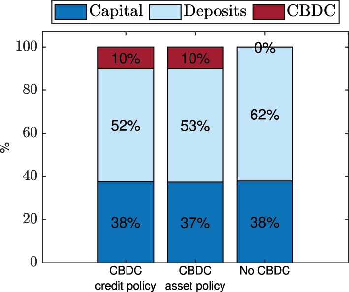
Households savings in steady state.
The consumption of bankers is lower due to lesser net worth and profitability of banks. Under CBDC with ‘asset policy’, the issuance of CBDC leads to a reduction in the size of the balance sheet, while under CBDC with ‘credit policy’ the lost deposit funding is replaced by central bank credit, leading to a balance sheet size that remains similar (Figure 2). Both policy scenarios strain profitability: while the issuance of CBDC under ‘credit policy’ reduces profitability through higher funding costs of central bank credit, the issuance of CBDC under ‘asset policy’ reduces net worth through a smaller balance sheet size. This smaller balance sheet, and hence the capital holdings of banks under CBDC with ‘asset policy’ is compensated by central bank capital holdings and the central bank takes over some of the capital investments which were previously held by banks (Figure 3). To summarise, both CBDC policy options do not change steady state aggregate output and welfare but only affect the distributions between households and banks.
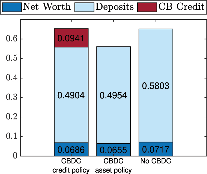
Bank funding in steady state.
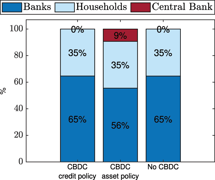
Capital allocation in steady state.
4.3 Financial Shocks Under a CBDC
The following section investigates the impact of a CBDC in response to an unanticipated 5 % shock to capital productivity that does not trigger a bank run. Figure 4 shows the response of key variables to the shock. Overall, the issuance of CBDC tends to reduce output losses, albeit only marginally. The slightly dampened impact on output can be explained by the stabilising effect of CBDC issuance on capital prices under both policy scenarios. Under CBDC with ‘credit policy’, capital prices are stabilised by refinancing bank funding with increased loans from the central bank. Under CBDC with asset policy capital prices are stabilised through increased capital holdings by the central bank that substitute for household capital holdings.
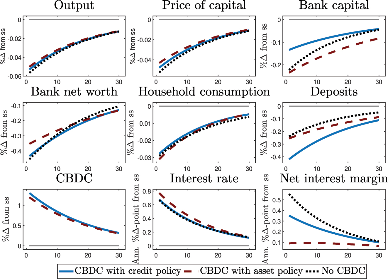
No-bank-run response to a 5 % shock to capital productivity.
The simulated shock to capital quality tightens the bank’s leverage constraint, forcing a reduction in bank capital. Under CBDC issuance with ‘asset policy’, bank capital and deposits fall similarly strong but more persistently than in the ‘no CBDC’ scenario. In contrast to the ‘no CBDC’ scenario, households do not have to fully absorb the reduction in bank capital but can also hold CBDC which increases in response to the shock. To complement the inflow in CBDC holdings on the balance sheet, the central bank increases its investments in bank capital. Those activities alleviate household managements costs and stabilise the price of capital which leads to a smaller drop in bank net worth than in the alternative scenarios.
Under CBDC issuance with ‘credit policy’, the decline in bank capital is smaller than under the alternative scenarios. The decrease in deposits that is replaced by CBDC is channelled back to the bank in the form of central bank credit, mitigating the drop in bank capital and stabilising the price of capital. However, central bank credit is provided at higher funding costs and leads to a similar decline in bank net worth as in the ‘no CBDC’ scenario. Nevertheless, the optimal funding structure of banks still shifts towards central bank credit because the increase in the bank’s interest margin is higher for loans than for deposits. This also explains why the decline in deposits is steeper than in the alternative scenarios.
In all scenarios, the decline in household consumption is similar, being least severe under ‘credit policy’, while the decline in bankers’ consumption is least severe under ‘asset policy’. Considering household and bank consumption jointly, the aggregated and discounted welfare across periods in response to the shock is higher under the CBDC scenarios (‘asset policy’: 4.9566, ‘credit policy’: 4.9573) than in the ‘no CBDC’ scenario (4.9546). Taking stock, CBDC issuance tends to mitigate the response to capital quality shocks by stabilising asset prices but which comes at the cost of larger deposit outflows. Appendix A presents variations in the calibration of the less established parameters δ Y and δ M in the CBDC interest rate rule, the capital management costs of the central bank α cb , as well as the leverage constraint for central bank credit to banks ω.
4.4 Bank Failures
Following on from Section 3.2 which distinguished between the different types of bank failures, this section investigates bank failures and the different equilibrium regions in the numerical example. Specifically, it addresses the questions: how large does a shock to the steady state have to be (i) for a self-fulfilling bank run equilibrium to emerge and enabling a bank failure due to illiquidity, and (ii) to cause a bank failure due to insolvency?
Figure 5 provides the answer to these questions by showing the equilibrium regions for the different policies in the context of the numerical example.[30] In the baseline case without CBDC, self-fulfilling bank runs become possible when capital productivity shocks exceed 2.5 %. When capital shocks exceed 8.04 %, all deposits are withdrawn regardless of the beliefs of other households and banks become insolvent. Including CBDC issuance in the model framework improves financial stability by postponing both types of bank failure to larger shocks. Under CBDC issuance with ‘asset policy’, self-fulfilling runs become possible when capital productivity shocks exceed 8.57 % and banks become insolvent at shock sizes above 11.3 %. Under CBDC issuance with ‘credit policy’, the lender of last resort measures prevent self-fulfilling runs in the baseline calibration, but not in general. At the same time, under CBDC issuance with ‘credit policy’, banks already become insolvent at shock sizes above 8.26 %, a region similar to the insolvency threshold of no CBDC issuance. The following subsections will further dissect the mechanisms at play for the equilibrium regions in the different policy scenarios.
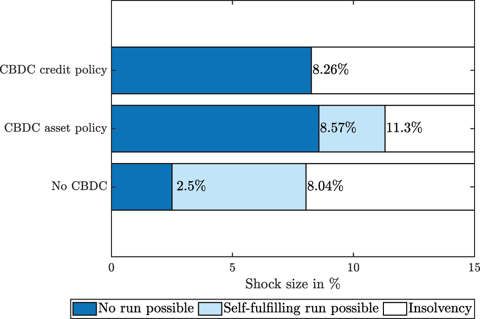
Shock sizes to steady state levels that are needed i) for the emergence of a self-fulfilling run, leading to default due to illiquidity and ii) for triggering a fundamental bank run, leading to insolvency in the period of the shock.
4.4.1 Bank Failures Due to Illiquidity
4.4.1.1 Bank Runs Without a CBDC
Figure 6 compares the bank run and no bank run scenarios after a 5 % shock to capital productivity in the case without CBDC issuance. As long as households believe that other households will not lose faith and run on the bank, the banking equilibrium prevails and the shock has the dynamics as displayed in Figure 4 (black solid lines in Figure 6 and black dotted lines in Figure 4). However, if households believe that the shock prompts others to withdraw their deposits, it triggers a bank run in the period of the shock (grey dashed lines in Figure 6).
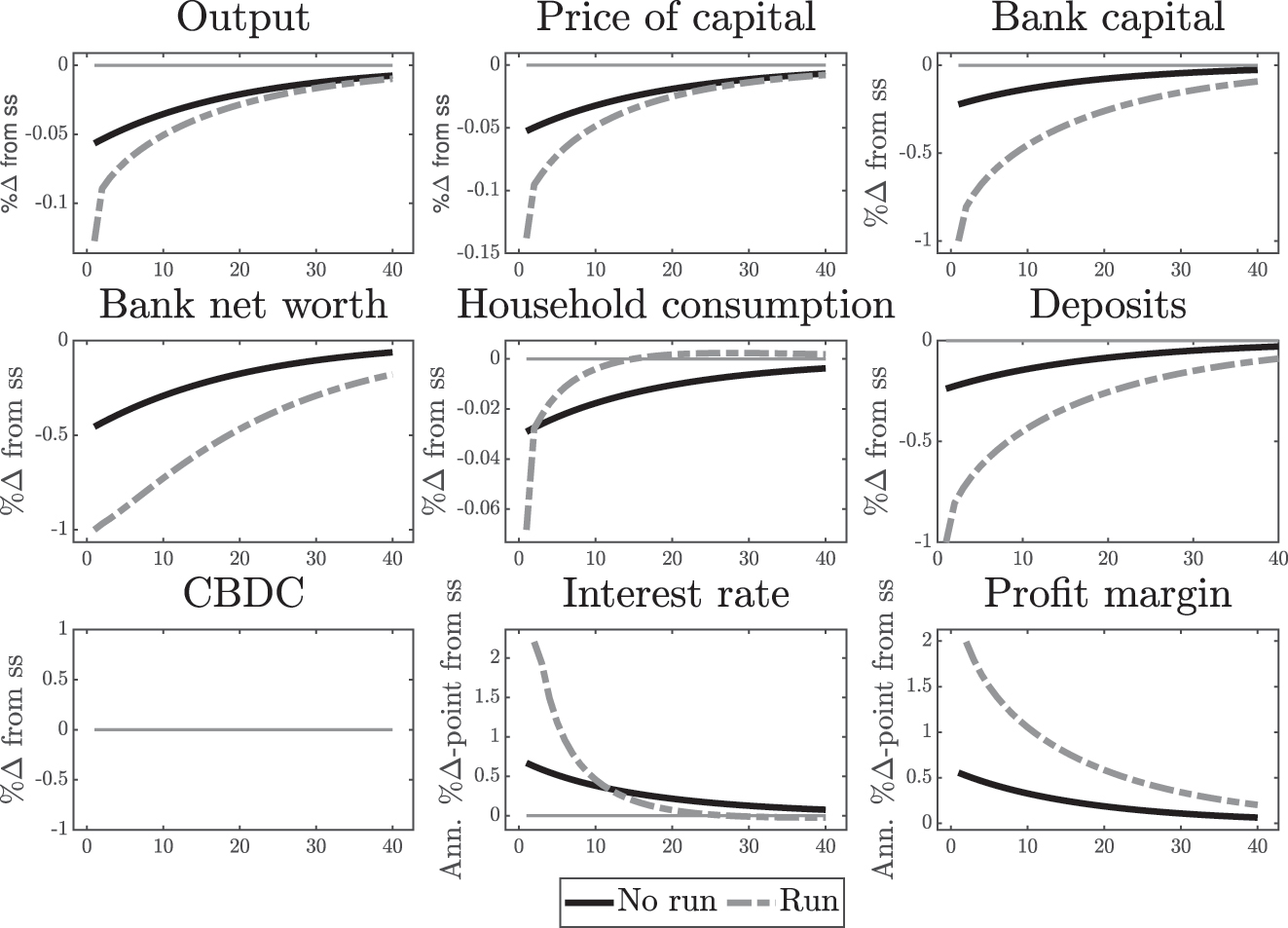
‘No CBDC scenario’ – 5 % shock to productivity with and without a bank run in the period of the shock.
The bank run leads to a complete withdrawal of deposits, forcing the banks to liquidate all their capital. All banks fail as their net worth is wiped out during the run. Only households are left to purchase capital and as they are less efficient than banks, they face increasing marginal costs for managing capital. Therefore, capital is sold at a fire-sale price, a price much lower than it would have been in the absence of a run. Overall, the bank run leads to a sharp drop in output and consumption. In the period after the bank run, the banking sector starts to recapitalise. Due to the reduced capital productivity and price, banks are initially able to earn high profit margins, leading to high interest rates and a rapid recovery.
4.4.1.2 Bank Runs Under CBDC with Asset Policy
CBDC issuance with ‘asset policy’ requires a much larger shock to enable the possibility of self-fulfilling runs. Figure 7 compares the bank run (light red dashed lines) and no bank run (red solid lines) scenarios after a 10 % shock to capital productivity. In response to the bank run, the price of capital falls sharply, although in relative terms less than in the ‘no CBDC’ scenario. The dampened decline in capital prices translates into relatively less severe output losses and consumption losses compared to the ‘no CBDC’ case, but still more severe than the no bank run scenario.
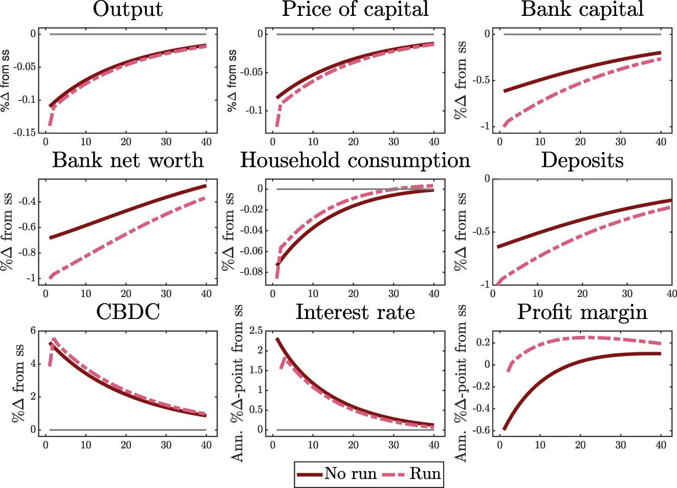
CBDC with asset policy scenario – 10 % shock to productivity with and without a bank run in the period of the shock.
The central bank’s asset purchases stabilise the fire-sale price of assets, thereby mitigating output losses in the bank run scenario. When withdrawing deposits from the bank, households can now hold both capital and CBDC. The additional option to hold CBDC makes the run less costly as households do not have to hold all their funds in the form of capital. Instead, some of the capital is also held by the central bank. Jointly holding the capital stock during the bank run stabilises the fire-sale price for two reasons: first, although the central bank is less efficient in managing capital than the bank, it is more efficient and faces lower capital management costs than households. Second, capital is held jointly by households and the central bank and, as capital management costs are convex, this further mitigates the overall efficiency losses of capital.
The stabilising influence of central bank asset purchases on the fire-sale price of capital is sufficiently large to fully cover deposit claims even in response to larger shocks and thereby postpones the occurrence of self-fulfilling bank runs. While a bank run under CBDC issuance with asset policy still leads to a welfare deterioration, the additional welfare loss is smaller which leads to a more resilient economy towards self-fulfilling runs.
4.4.1.3 Bank Runs Under CBDC with Credit Policy
The issuance of CBDC with ‘credit policy’ increases the threshold for self-fulfilling runs further. In the baseline calibration, there is no region in which the banking and the bank run equilibrium coexist. This result rests on the assumption that the central bank does not participate in self-fulfilling bank runs but only withdraws funding once the bank is insolvent.[31]
There are two forces that jointly impede the occurrence of bank runs under CBDC with ‘credit policy’. First, in the event of a bank run, only a fraction of the bank’s liabilities are withdrawn, as both deposits and central bank credit are on the bank’s balance sheet. Therefore, the fire-sale price of assets needs to cover only the share of liabilities that are deposits as the central bank does not engage in the bank run. In this way, central bank credit provides the bank with a stable funding source which creates an additional buffer on the bank’s balance sheet. This additional central bank credit buffer results in a lower share of assets that would be withdrawn in a bank run scenario and makes the funding outflow easier to absorb. The larger the pre-run central bank credit holdings are, the higher the hurdle for the emergence of a self-fulfilling bank run. Second, instead of withdrawing funds, the central bank simultaneously provides the bank with additional liquidity in the amount of inflows into CBDC. The continued credit provision enables the bank to invest in capital even in case of a bank run. With the bank being more efficient in managing capital, this greatly stabilises the capital price. Acting as lender of last resort, the central bank provision of credit further impedes the emergence of bank runs. Those two forces break the ‘doom-loop’ of self-fulfilling runs in the baseline calibration.
How can banks under CBDC with ‘credit policy’ become insolvent without opening the possibility for self-fulfilling runs? As described above, the price threshold
Overall, by interceding as lender of last resort with the funds from CBDC, the central bank altogether eliminates the possibility of a run in the context of the numerical example. However, this does not preclude self-fulfilling bank runs under credit policy in the general setting. Self-fulfilling bank runs under CBDC with credit policy are possible under alternative calibrations.
Which of the two channels preventing the bank run under the baseline calibration is stronger and what are the implications of reducing both forces, individually and jointly? The first force works via the share of credit on the bank’s liabilities in the period before the bank run. Reducing δ0 in the central bank’s CBDC rule to δ0 = 1.01015 diminishes central bank credit in steady state to almost zero, with Lst.st. = 0.0005 (instead of Lst.st. = 0.0941 under the baseline calibration with δ0 = 1.0194). Muting the first channel is not sufficient to enable self-fulfilling bank runs before the insolvency threshold. The second channel of providing central bank credit via CBDC inflows is sufficiently strong to still prevent the bank run from the outset. The second channel can be relaxed by increasing the reaction to CBDC demand in the CBDC rule to δ M to disincentivise CBDC uptake. Setting δ M = 0.5 (instead of δ M = 0.1 under the baseline calibration), self-fulfilling bank runs become possible from shock sizes above 6.3 %. Relaxing both forces jointly, with δ0 = 1.01015 and δ M = 0.5, enables self-fulfilling bank runs already from shock sizes above 2.9 %.
4.4.1.4 The Role of Friction for the Emergence of Self-Fulfilling Runs
Both types of CBDC issuance – with ‘asset policy’ and ‘credit policy’ – delay the emergence of the bank run equilibrium to larger shocks by reducing frictions during a bank run. This stabilises the fire-sale price of assets, mitigates welfare losses and makes banks runs more difficult to emerge. The contributions of the different model frictions to the emergence of bank runs are examined in more detail below.
The main friction that makes bank runs costly is the capital management cost of households α. Reducing the household capital management costs to almost zero with α = 0.001 (α = 0.008 in the baseline calibration) delays the emergence of self-fulfilling runs in the ‘no CBDC’ scenario to the brink of insolvency at shocks above 21.9 % (vs. 2.5 % under the baseline calibration). Conversely, increasing capital management costs to α = 0.015 in the scenario without CBDC enables a bank run equilibrium already in steady state in the absence of any shocks.
While additional frictions in the CBDC scenarios also play a role for the emergence of bank runs, they are not as central as household capital management costs α and the parameters of the CBDC reaction rule. In the scenario of CBDC issuance with ‘asset policy’, capital management costs of the central bank are introduced as additional friction. Reducing the central bank’s capital management costs to α cb = 0.001 (instead of α cb = 0.004 in the baseline calibration) delays the emergence of self-fulfilling runs from shocks above 8.6 % under the baseline calibration to shocks above 9.7 %. Conversely, setting central bank capital management costs to the capital management costs of the households with α cb = 0.008 reduces the shock threshold for the emergence of bank runs to shocks above 7.7 %. In the CBDC scenario with ‘credit policy’, the leverage constraint for central bank credit ω is introduced as an additional friction. Setting ω = 1 removes the leverage constraint but increases the costs of central bank credit which leads to the possibility of self-fulfilling bank runs at shocks above 2.1 %. Conversely, setting ω = 0 leads to the same leverage constraint but also to the same funding costs as on deposits. Similarly to the baseline calibration, this does not open up the possibility of self-fulfilling runs before the insolvency threshold.
Moreover, bank runs are not anticipated. How would the results change if bank runs were anticipated, for example as in Gertler and Kiyotaki (2015) or Gertler, Kiyotaki, and Prestipino (2016a)? Accounting for the possibility of bank failures would lead to a risk premium on deposits and increase bank funding costs. As the introduction of CBDC in the model framework makes bank runs less likely by delaying their occurrence to larger shocks, the risk premium on deposits would decrease in the presence of CBDC. Therefore, introducing anticipation of bank runs into the analysis would not materially change the insights of this analysis and results would be strengthened further. In addition, allowing for anticipation of bank failures, CBDC would be more favourable for the profitability of banks as the introduction of CBDC would reduce the risk premium and thus the deposit funding costs and therefore further mitigate financial fragility.
4.4.2 Bank Failures Due to Insolvency
Figure 8 displays the evolution of deposits to increasing shock sizes under the different policy scenarios. Banks become insolvent in response to a shock when the non-fire-sale value of assets becomes smaller than the liabilities. Thus, the conditions for a default due to illiquidity and default due to insolvency only differ in the price of capital for the ‘no CBDC’ and CBDC with ‘asset policy’ scenarios. For CBDC with ‘credit policy’, the conditions for bank failure due to illiquidity and insolvency also differ in the assets that are taken into account. While the central bank does not engage in self-fulfilling runs and the fire-sale value of assets only needs to cover deposits, the central bank credit claims are taken into account in the calculation of the insolvency conditions.
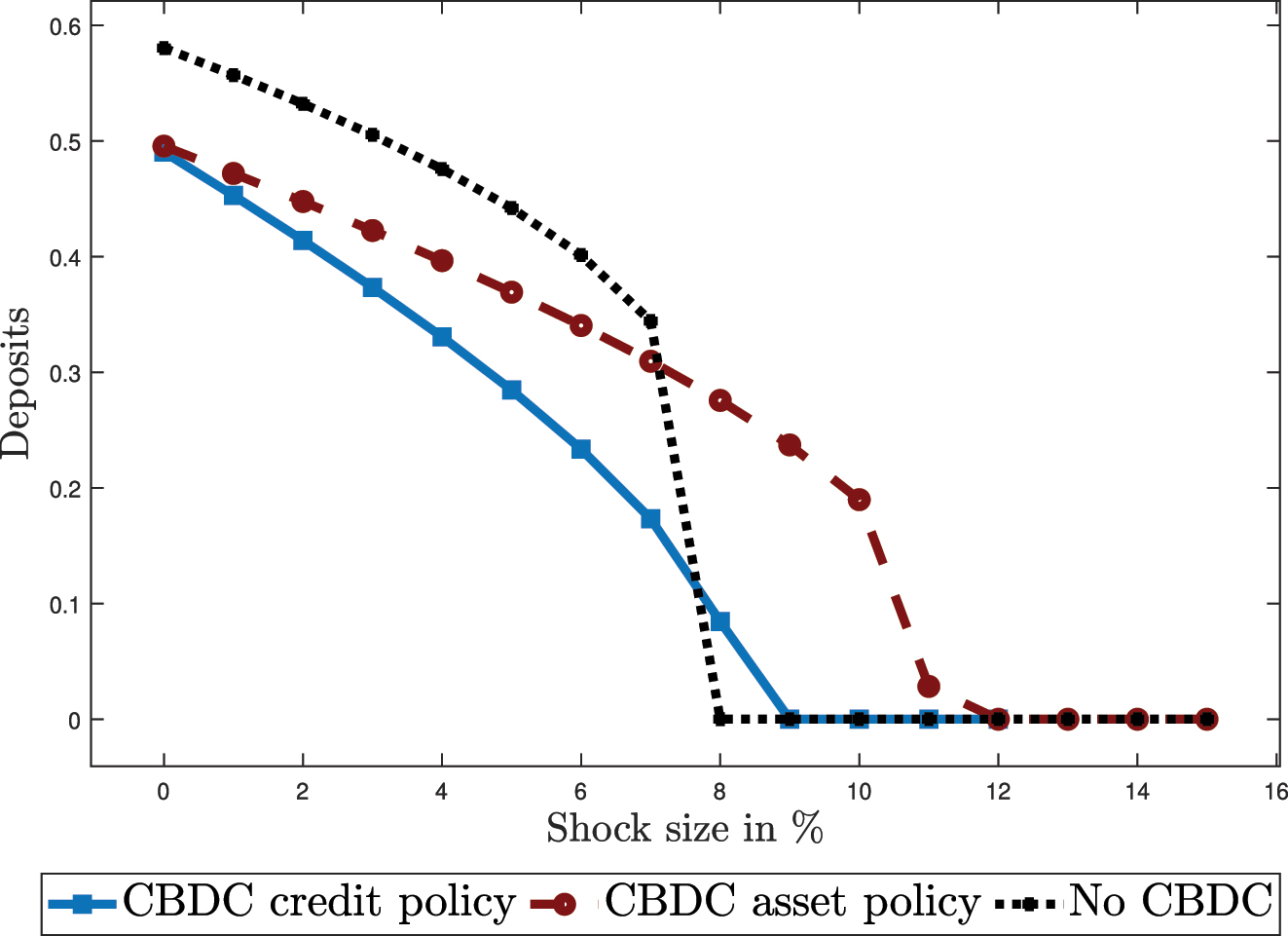
Evolution of deposits in the period of the shock with increasing capital shock sizes under the different policy scenarios and without emergence of self-fulfilling runs.
The size of shocks that thrust banks into insolvency under CBDC with ‘credit policy’ is similar but a bit later than the scenario without CBDC. While in both scenarios the overall balance sheet size is similar, the stabilisation of capital prices under CBDC with ‘credit policy’ leads to a deferral of insolvency to slightly larger shock. In contrast, the shock size that triggers insolvency under CBDC with ‘asset policy’ is substantially larger. The higher insolvency threshold can be explained by the smaller bank balance sheet under CBDC with ‘asset policy’ and also by the stabilisation of the capital price.
To summarise, under both policy scenarios CBDC affects the equilibrium regions in a way that supports financial stability. Under CBDC with ‘asset policy’, the emergence of both bank run types is postponed to substantially larger shock. Under CBDC with ‘credit policy’, the possibility of self-fulfilling runs does not arise in the baseline calibration, while insolvency is triggered at a similar shock size as in the ‘no CBDC’ scenario.
5 Conclusion
One of the main concerns about a CBDC is its disintermediating effect on the banking sector and especially the increased risk of a bank run in times of crisis. This paper analyses the impact of CBDC on financial stability as an extension of the dynamic bank run model with a financial accelerator by Gertler and Kiyotaki (2015).
CBDC issuance creates an additional type of liability on the central bank balance sheet which will lead to further balance sheet adjustments. In the model analysis, I account for the potentially different impact of these balance sheet adjustments by analysing CBDC issuance in the context of two different asset side policies: by granting loans to banks (CBDC with ‘credit policy’) and by purchasing capital (CBDC with ‘asset policy’).
The stylised model analysis offers several insights: in the steady state, a CBDC does not affect output and welfare. Instead, it affects the composition of household savings, bank funding and capital investment, ultimately reducing bank profits. In response to shocks that do not trigger a bank run, the issuance of CBDC does not exacerbate, but rather tends to mitigate, output and welfare losses by stabilising asset prices. At the same time, the presence of CBDC also leads to larger deposit outflows. Most importantly, the stabilisation of asset prices improves financial stability by deferring the emergence of bank failures due to illiquidity (caused by self-fulfilling runs) and bank failures due to insolvency to larger shocks. Overall, I find that a CBDC strains the banking sector in normal times by reducing deposits and net worth. Yet, contrary to prevailing concerns, CBDC improves financial stability in times of crisis by stabilising capital prices through asset-side adjustments that follow CBDC issuance.
This analysis is carried out in a stylised setting that abstracts from several features that could be considered in future research. For instance by: (i) bringing the analysis from a real to a nominal setting that allows for inflation dynamics and conventional monetary policy, (ii) introducing a richer financial sector and embedding a more complex structure of the central bank balance sheet that includes reserves, cash, government bonds and a collateral framework, (iii) incorporating the function of money as a medium of exchange into the analysis and (iv) allowing for richer dynamics and frictions at firm level.
Acknowledgments
For helpful comments, I would like to thank two anonymous referees, Lukas Altermatt, Ulrich Bindseil, Michael Burda, Lukas Gehring, Rouven Geismar, Petra Gerlach, Jonas Gross, Frank Heinemann, Jonathan Schiller, as well as participants at seminars and conferences organised by the ECB, Verein für Socialpolitik, TU Berlin, HU Berlin, University of Basel and Ruhr Graduate School in Economics. Support by Deutsche Forschungsgemeinschaft through CRC TRR 190 (project number 280092119) is gratefully acknowledged. The views expressed are those of the author which do not necessarily reflect those of the ECB, the author is not part of the ECB’s digital euro project team and most of the project was done at the TU Berlin before joining the ECB.
Appendix A: Comparison to Alternative Model Specifications
Most parameter values for the simulation are adopted from Gertler and Kiyotaki (2015). However, there are a few parameters that have been newly introduced and are less established in the literature. This section presents insights from: (i) varying the dynamic coefficients δ Y and δ M in the CBDC interest rate rule; (ii) varying the capital management costs of the central bank α cb ; and (iii) varying the leverage constraint for central bank credit to banks ω.
Overall, if the CBDC interest rate rule is more responsive to output fluctuations from steady state, this leads to a stronger stabilisation of output, consumption, capital prices, and bank net worth. Such stabilisation comes at the cost of higher deposit disintermediation and a larger increase in CBDC, also resulting in a larger central bank balance sheet. In contrast, a stronger response to CBDC demand makes the CBDC interest rate less attractive and leads to stronger automatic stabilisation of CBDC issuance, which in turn comes at the cost of lower stabilisation in output and capital prices.
The same mechanisms explain the optimal values of δ Y and δ M : the optimal δ Y that would maximise welfare (aggregate discounted total consumption) in response to a capital quality shock would be as high as possible, whereas the optimal δ M would be as low as possible. However, these welfare considerations do not take into account the negative implications of excessive central bank intervention in response to a shock, such as potential moral hazard side effects.
Relaxing the assumptions about the central bank’s capital management costs in case of CBDC with ‘asset policy’, and the leverage constraint for central bank credit to banks in the case of CBDC with ‘credit policy’, tends to lead to a higher effectiveness of central bank measures (i.e. a higher stabilisation and smaller increases in CBDC and the central bank balance sheet). Yet, one may question how reasonable it would be to fully relax those assumptions. The opposite picture emerges when these assumptions are further restricted. Although, overall the impact of variations is relatively small, especially for variations in capital management costs under CBDC with ‘asset policy’.
Appendix A.1: Varying CBDC Rule Parameters
The following section investigates how the response to a capital productivity shock changes, varying the two coefficients δ
Y
and δ
M
in the CBDC interest rate rule
The coefficient δ Y captures the reaction strength of the CBDC interest rate rule to fluctuations in output from its steady state value. Figures 9 and 10 display variations in δ Y in the ‘credit policy’ and ‘asset policy’ scenario. Compared to the baseline calibration (solid lines, following the calibration of Minesso, Mehl, and Stracca 2022), δ Y is doubled to 0.52 (higher output stabilisation, dashed lines) and halved to 0.13 (lower output stabilisation, dotted lines). Variations in δ Y have the same qualitative implications for CBDC issuance with ‘credit policy’ and ‘asset policy’: a higher response to output fluctuations increases the stabilisation of output, consumption, the price of capital, and bank net worth. Yet, this comes at the cost of a higher deposit disintermediation and a greater increase in CBDC issuance. The effects are reversed in the case of a lower responsiveness to output fluctuations i.e. lower stabilisation but lower disintermediation.
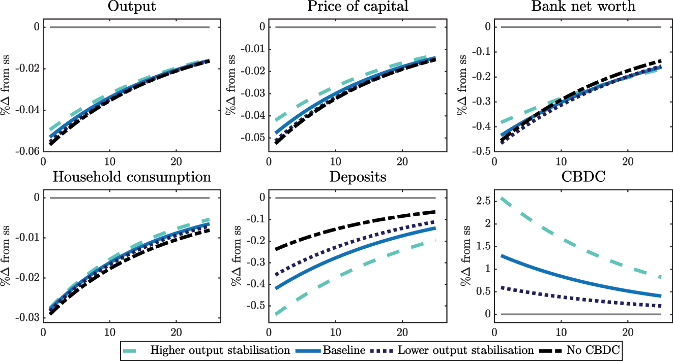
Response to a 5 % shock to productivity under CBDC with ‘credit policy’ for high and low CBDC rule output coefficient δ Y .
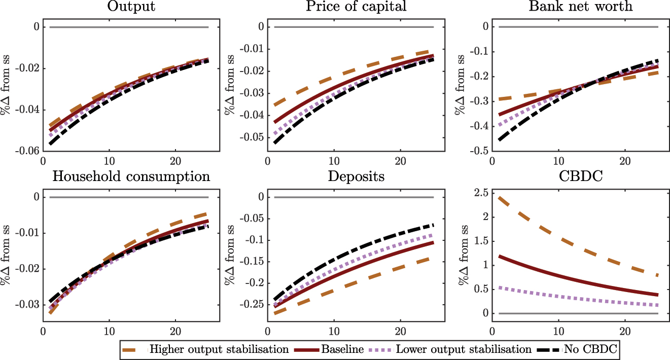
Response to a 5 % shock to productivity under CBDC with ‘asset policy’ for high and low CBDC rule output coefficient δ Y .
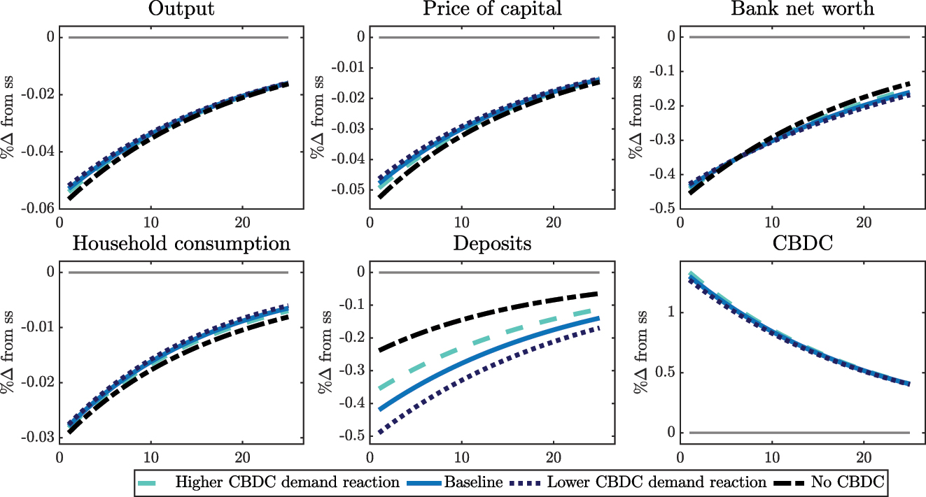
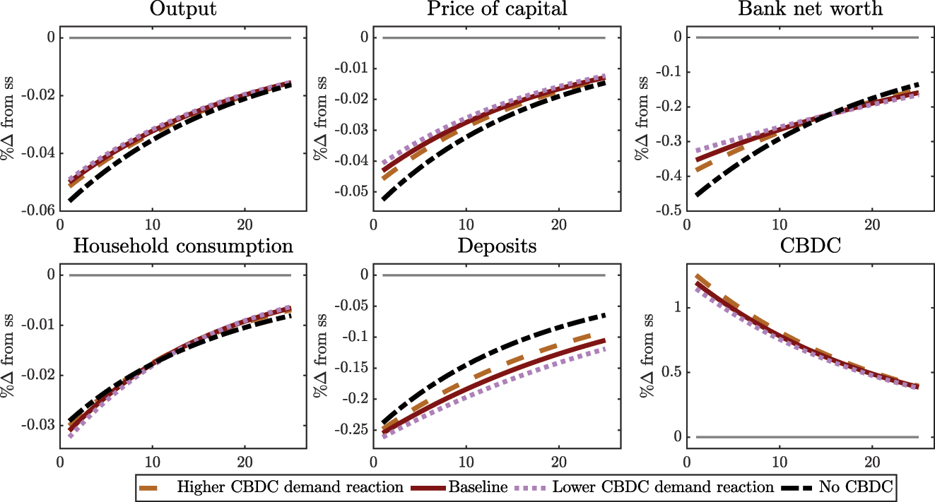
The coefficient δ M captures the responsiveness of the CBDC interest rate rule to CBDC demand and thereby stabilising fluctuations in CBDC. Figures 11 and 12 show variations in δ M in the ‘credit policy’ and ‘asset policy’ scenario. Compared to the baseline calibration (solid lines) of δ M = 0.1, δ M is increased to 0.15 (higher CBDC demand response, dashed lines) and reduced to 0.075 (lower CBDC demand response, dotted lines). Variations in δ M lead to similar observations as the variations in δ Y and have again have the same qualitative implications for CBDC issuance with ‘credit policy’ and ‘asset policy’. Making the CBDC interest rate rule less attractive in response to increased CBDC demand (i.e. a higher CBDC demand response) leads to a less stabilisation, but also to a smaller increase in CBDC supply (and vice versa). However, the difference in the variations is relatively small, except for the implications on the deposit response where the differences are most pronounced.
Response to a 5 % shock to productivity under CBDC with ‘credit policy’ for high and low CBDC rule CBDC demand coefficient δ M
Response to a 5 % shock to productivity under CBDC with ‘asset policy’ for high and low CBDC rule CBDC demand coefficient δ M .
Appendix A.2: Varying CBDC Credit and Asset Policy Assumptions
The following section investigates how the response to a capital productivity shock changes, varying the two additional assumptions underlying CBDC issuance with ‘credit policy’ and ‘asset policy’.
For CBDC issuance with ‘credit policy’, it is assumed that the leverage constraint of central bank credit to banks is less binding than for deposits, due to superior supervisory powers and collateral requirements. Figure 13 displays variations in the relative strength of the leverage constraint
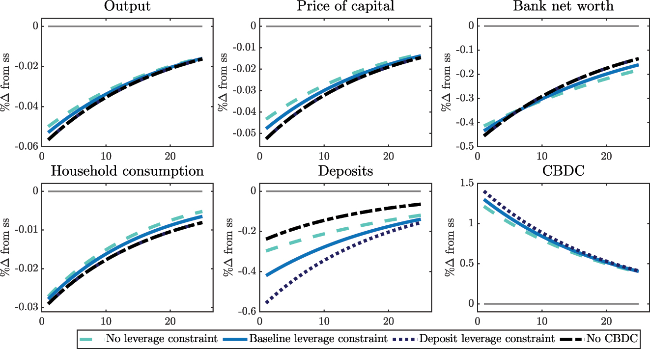
Response to a 5 % shock to productivity under CBDC with credit policy and varying leverage constraint for central bank credit.
Similarly, for CBDC with ‘asset policy’, the central bank is assumed to face lower capital management costs than households, but which are of the same functional form
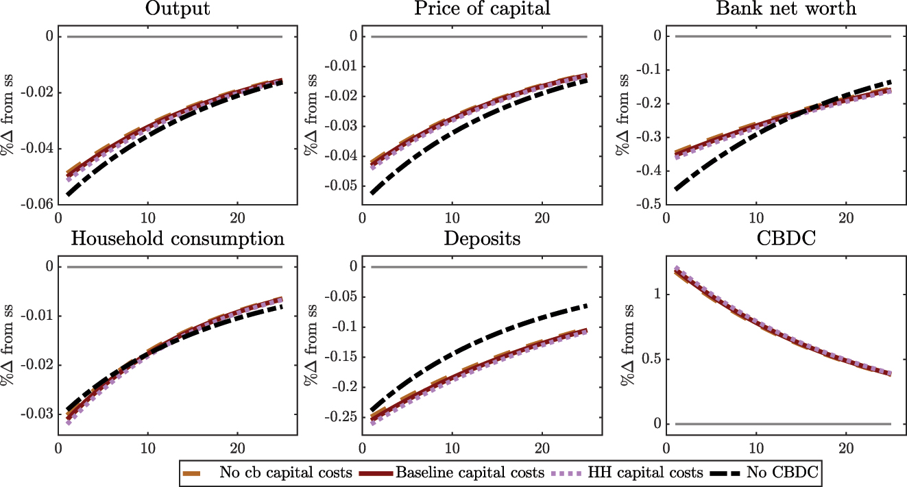
Response to a 5 % shock to productivity under CBDC with ‘asset policy’ and varying central bank capital management costs.
Appendix B: Optimisation Problem of the Banker
General optimisation: The banker chooses
The objective and constraints of the bank are subject to constant returns to scale; thus, they can be made independent of the total level of net worth by expressing the problem in terms of per unit of net worth. To make the maximisation problem independent of its initial conditions, equation (21) needs to be expressed in terms of per unit of net worth. For this, the evolution of net worth (5) is combined with the flow of funds constraint (4) and reformulated such that
where
Likewise, we can then express the value function as:
where Ωt+1 is the weighted average of the discounted marginal value of net worth to exiting and to remaining bankers. Ψ is the franchise value of the bank per unit of asset and can thus be interpreted as Tobin’s q ratio. Similarly, the flow of funds constraint (4) can be inserted into the incentive constraint (7) and expressed in terms of per unit of net worth:
Finally, the reformulated optimisation problem is choosing leverage (i.e. deposits and credit per unit of net worth
This leads to the Lagrangian function
with the Kuhn Tucker conditions
To show that the incentive constraint must be binding, assume conversely that the constraint is slack and thus λ
t
= 0: this would imply for equations (26)
yielding the following optimality conditions:
Optimisation under ‘asset policy’: The above setting is the more general one and applies to both, the scenario with ‘credit policy’ and ‘asset policy’. However, under the ‘asset policy’ scenario, the banker’s problem is simplified as the central bank does not provide credit and therefore l
t
= 0. In this case, the bank’s optimisation problem reduces to the case in GK15, since deposits are the only type of leverage and the bank simply chooses deposits per unit of net worth
Appendix C: Overview of Equations in the Different Models
Overview of equations in the different policy scenarios.
| Description | Equation | CBDC credit policy | CBDC asset policy | No CBDC |
|---|---|---|---|---|
| Households | ||||
|
|
||||
| Deposit euler |
|
✓ | ✓ | ✓ |
| CBDC euler |
|
✓ | ✓ | |
| Capital euler |
|
✓ | ✓ | ✓ |
|
|
||||
| Banking sector | ||||
|
|
||||
| Balance sheet |
|
✓ | ||
|
|
✓ | ✓ | ||
| Net worth |
|
✓ | ||
|
|
✓ | ✓ | ||
| Max problem |
|
✓ | ||
|
|
||||
|
|
✓ | ✓ | ||
| with
|
||||
| Leverage constraint |
|
✓ | ||
|
|
✓ | ✓ | ||
| Leverage combination |
|
✓ | ||
|
|
||||
| Central bank | ||||
|
|
||||
| CB balance |
|
✓ | ||
|
|
✓ | |||
| CBDC interest rate |
|
✓ | ✓ | |
| CB lending | L t = M t | ✓ | ||
| CB capital |
|
✓ | ||
|
|
||||
| Aggregation and market clearing | ||||
|
|
||||
| Total capital |
|
✓ | ✓ | |
|
|
✓ | |||
| Total output |
|
✓ | ✓ | |
|
|
✓ | |||
| = Z t + z t W h + W b | ||||
Overview of bank run equilibrium equations.
| Description | Equation | CBDC credit policy | CBDC asset policy | No CBDC |
|---|---|---|---|---|
| Households | ||||
|
|
||||
| CBDC euler |
|
✓ | ✓ | |
| Capital euler |
|
✓ | ✓ | ✓ |
|
|
||||
| Banking sector | ||||
|
|
||||
| Balance sheet |
|
✓ | ||
|
|
||||
| Central bank | ||||
|
|
||||
| CB balance |
|
✓ | ||
|
|
✓ | |||
| CBDC interest rate |
|
✓ | ✓ | |
| CB lending | L t = M t | ✓ | ||
| CB capital |
|
✓ | ||
|
|
||||
| Aggregation and market clearing | ||||
|
|
||||
| Total capital |
|
✓ | ||
|
|
✓ | |||
|
|
✓ | |||
| Total output |
|
✓ | ✓ | |
|
|
✓ | |||
References
Adalid, R., Á. Álvarez-Blázquez, K. Assenmacher, L. Burlon, M. Dimou, C. López-Quiles, N. M. Fuentes, et al.. 2022. “Central Bank Digital Currency and Bank Intermediation.” ECB Occasional Paper (293).10.2139/ssrn.4108346Search in Google Scholar
Ahnert, T., K. Assenmacher, P. Hoffmann, A. Leonello, C. Monet, and D. Porcellacchia. 2022. “The Economics of Central Bank Digital Currency.” ECB Working Paper No 2713.10.2139/ssrn.4192178Search in Google Scholar
Ahnert, T., P. Hoffmann, A. Leonello, and D. Porcellacchia. 2023. “CBDC and Financial Stability.” ECB Working Paper No 2783.10.2139/ssrn.4361136Search in Google Scholar
Andolfatto, D. 2021. “Assessing the Impact of Central Bank Digital Currency on Private Banks.” The Economic Journal 131 (634): 525–40. https://doi.org/10.1093/ej/ueaa073.Search in Google Scholar
Assenmacher, K., A. Berentsen, C. Brand, and N. Lamersdorf. 2021. “A Unified Framework for CBDC Design: Remuneration, Collateral Haircuts and Quantity Constraints.” ECB Working Paper No 2578.10.2139/ssrn.3896787Search in Google Scholar
Assenmacher, K., L. Bitter, and A. Ristiniemi. 2023. “CBDC and Business Cycle Dynamics in a New Monetarist New Keynesian Model.” ECB Working Paper No 2811.10.2139/ssrn.4442377Search in Google Scholar
Bagehot, W. 1873. Lombard Street: A Description of the Money Market. London: HS King.Search in Google Scholar
Bank for International Settlements. 2018. “Central Bank Digital Currencies.” In Committee on Payments and Market Infrastructures Markets Committee and Markets Committee. Basel: Bank for International Settlements.Search in Google Scholar
Bank for International Settlements. 2020. BIS Statistics Explorer: Table CT2: Banknotes and Coins in Circulation, Value as Percentage of GDP, Technical Report. Basel: Bank for International Settlements. https://stats.bis.org/statx/srs/table/CT2?c=p=2018m=3 (accessed December 15, 2021).Search in Google Scholar
Bank of England, and HM Treasury. 2023. “The Digital Pound: A New Form of Money for Households and Businesses?” Consultation Paper, February.Search in Google Scholar
Barker, J., D. Bholat, and R. Thomas. 2017. “Central Bank Balance Sheets: Past, Present and Future.” Bank Underground Blog, Bank of England, https://bankunderground.co.uk/2017/07/03/central-bank-balance-sheets-past-present-and-future/ (accessed August 11, 2024).10.2139/ssrn.2996632Search in Google Scholar
Barontini, C., and H. Holden. 2019. “Proceeding with Caution – A Survey on Central Bank Digital Currency.” BIS Papers No 101.Search in Google Scholar
Barrdear, J., and M. Kumhof. 2022. “The Macroeconomics of Central Bank Digital Currencies.” Journal of Economic Dynamics and Control 142: 104148. https://doi.org/10.1016/j.jedc.2021.104148.Search in Google Scholar
Bindseil, U. 2019. “Central Bank Digital Currency: Financial System Implications and Control.” International Journal of Political Economy 48 (4): 303–35. https://doi.org/10.1080/08911916.2019.1693160.Search in Google Scholar
Bindseil, U., F. Panetta, and I. Terol. 2021. “Central Bank Digital Currency: Functional Scope, Pricing and Controls.” ECB Occasional Paper No 286.10.2139/ssrn.3975939Search in Google Scholar
Brunnermeier, M. K., and D. Niepelt. 2019. “On the Equivalence of Private and Public Money.” Journal of Monetary Economics 106: 27–41. https://doi.org/10.1016/j.jmoneco.2019.07.004.Search in Google Scholar
Burlon, L., C. Montes-Galdon, M. A. Muñoz, and F. Smets. 2022. “The Optimal Quantity of CBDC in a Bank-Based Economy.” ECB Working Paper No. 2689.10.2139/ssrn.4175853Search in Google Scholar
Carney, M. 2018. “The Future of Money.” In Speech at the Inaugural Scottish Economics Conference, Edinburgh University, 2 March 2018. London: Bank of England. https://www.bankofengland.co.uk/-/media/boe/files/speech/2018/the-future-of-money-speech-by-mark-carney.pdf?la=enhash=A51E1C8E90BDD3D071A8D6B4F8C1566E7AC91418 (accessed August 11, 2024).Search in Google Scholar
Cavallino, P., and F. De Fiore. 2020. “Central Banks’ Response to Covid-19 in Advanced Economies.” BIS Bulletin 21.Search in Google Scholar
Chapman, J., J. Chiu, M. Davoodalhosseini, J. H. Jiang, F. Rivadeneyra, and Y. Zhu. 2023. “Central Bank Digital Currencies and Banking: Literature Review and New Questions.” Bank of Canada Staff Discussion Papers (2023–4).Search in Google Scholar
Chiu, J., S. M. Davoodalhosseini, J. Jiang, and Y. Zhu. 2023. “Bank Market Power and Central Bank Digital Currency: Theory and Quantitative Assessment.” Journal of Political Economy 131 (5): 1213–48. https://doi.org/10.1086/722517.Search in Google Scholar
Diamond, D. W., and P. H. Dybvig. 1983. “Bank Runs, Deposit Insurance, and Liquidity.” Journal of Political Economy 91 (3): 401–19. https://doi.org/10.1086/261155.Search in Google Scholar
ECB. 2020. Report on a Digital Euro. Frankfurt am Main: European Central Bank.Search in Google Scholar
Fernández-Villaverde, J., D. Sanches, L. Schilling, and H. Uhlig. 2021. “Central Bank Digital Currency: Central Banking for All?” Review of Economic Dynamics 41: 225–42. https://doi.org/10.1016/j.red.2020.12.004.Search in Google Scholar
Fraschini, M., L. Somoza, and T. Terracciano. 2021. “Central Bank Digital Currency and Quantitative Easing.” Swiss Finance Institute Research Paper (21–25).10.2139/ssrn.3804966Search in Google Scholar
Gertler, M., and P. Karadi. 2013. “QE 1 vs. 2 vs. 3 …: A Framework for Analyzing Large-Scale Asset Purchases as a Monetary Policy Tool.” International Journal of Central Banking 9 (1): 5–53.Search in Google Scholar
Gertler, M., and N. Kiyotaki. 2010. “Financial Intermediation and Credit Policy in Business Cycle Analysis.” In Handbook of Monetary Economics, 3, 547–99. Amsterdam: Elsevier.10.1016/B978-0-444-53238-1.00011-9Search in Google Scholar
Gertler, M., and N. Kiyotaki. 2015. “Banking, Liquidity, and Bank Runs in an Infinite Horizon Economy.” American Economic Review 105 (7): 2011–43. https://doi.org/10.1257/aer.20130665.Search in Google Scholar
Gertler, M., N. Kiyotaki, and A. Prestipino. 2016a. “Anticipated Banking Panics.” American Economic Review 106 (5): 554–9. https://doi.org/10.1257/aer.p20161089.Search in Google Scholar
Gertler, M., N. Kiyotaki, and A. Prestipino. 2016b. “Wholesale Banking and Bank Runs in Macroeconomic Modeling of Financial Crises.” Handbook of Macroeconomics 2: 1345–425. https://doi.org/10.1016/bs.hesmac.2016.03.009.Search in Google Scholar
Gertler, M., N. Kiyotaki, and A. Prestipino. 2020. “A Macroeconomic Model with Financial Panics.” The Review of Economic Studies 87 (1): 240–88. https://doi.org/10.1093/restud/rdz032.Search in Google Scholar
Gross, J., and J. Schiller. 2020. “A Model for Central Bank Digital Currencies: Do CBDCs Disrupt the Financial Sector?” Working paper available on SSRN.10.2139/ssrn.3721965Search in Google Scholar
Group of Central Banks. 2020. “Central Bank Digital Currencies: Foundational Principles and Core Features, Report 1, Series of Collaborations from a Group of Central Banks.” https://www.bis.org/publ/othp33.pdf (accessed August 11, 2024).Search in Google Scholar
Juks, R. 2018. “When a Central Bank Digital Currency Meets Private Money: Effects of an e-Krona on Banks.” Sveriges Riksbank Economic Review 2018:3 Special issue on the e-krona.Search in Google Scholar
Keister, T., and C. Monnet. 2022. “Central Bank Digital Currency: Stability and Information.” Journal of Economic Dynamics and Control 142: 104501. https://doi.org/10.1016/j.jedc.2022.104501.Search in Google Scholar
Keister, T., and D. Sanches. 2023. “Should Central Banks Issue Digital Currency?” The Review of Economic Studies 90 (1): 404–31. https://doi.org/10.1093/restud/rdac017.Search in Google Scholar
Kim, Y. S., and O. Kwon. 2023. “Central Bank Digital Currency and Financial Stability.” Journal of Money, Credit and Banking 55 (1): 297–321. https://doi.org/10.1111/jmcb.12913.Search in Google Scholar
Kosse, A., and I. Mattei. 2023. “Making Headway-Results of the 2022 BIS Survey on Central Bank Digital Currencies and Crypto.” BIS Papers.Search in Google Scholar
Kumhof, M., and C. Noone. 2021. “Central Bank Digital Currencies – Design Principles for Financial Stability.” Economic Analysis and Policy 71: 553–72. https://doi.org/10.1016/j.eap.2021.06.012.Search in Google Scholar
Lucas, D. T. 2022. “Central Bank Digital Currencies and Financial Stability in a Modern Monetary System.” GEAR Working Paper 2022-01.Search in Google Scholar
Mancini-Griffoli, T., M. S. Martinez Peria, I. Agur, A. Ari, J. Kiff, A. Popescu, and C. Rochon. 2018. “Casting Light on Central Bank Digital Currency.” IMF Staff Discussion Note November 2018 SDN/18/08.10.5089/9781484384572.006Search in Google Scholar
Meaning, J., B. Dyson, J. Barker, and E. Clayton. 2018. “Broadening Narrow Money: Monetary Policy with a Central Bank Digital Currency.” Bank of England Staff Working Paper No. 724.10.2139/ssrn.3180720Search in Google Scholar
Meller, B., and O. Soons. 2023. “Know Your (Holding) Limits: CBDC, Financial Stability and Central Bank Reliance.” De Nederlandsche Bank Working Paper No 771.10.2139/ssrn.4543369Search in Google Scholar
Minesso, M. F., A. Mehl, and L. Stracca. 2022. “Central Bank Digital Currency in an Open Economy.” Journal of Monetary Economics 127: 54–68. https://doi.org/10.1016/j.jmoneco.2022.02.001.Search in Google Scholar
Muñoz, M. A., and O. Soons. 2024. “Public Money as a Store of Value, Heterogeneous Beliefs and Banks: Implications of CBDC.” ECB Working Paper No 2801.10.2139/ssrn.4728657Search in Google Scholar
Niepelt, D. 2020. “Reserves for All? Central Bank Digital Currency, Deposits, and Their (Non)-Equivalence.” International Journal of Central Banking 16 (3): 211–38.Search in Google Scholar
Panetta, F. 2022. “The Digital Euro and the Evolution of the Financial System.” In Introductory Statement at the Committee on Economic and Monetary Affairs of the European Parliament. Frankfurt am Main: European Central Bank. https://www.ecb.europa.eu/press/key/date/2022/html/ecb.sp220615 0b859eb8bc.en.html (accessed August 11, 2024).Search in Google Scholar
Pattipeilohy, C. 2016. “A Comparative Analysis of Developments in Central Bank Balance Sheet Composition.” BIS Working Paper No 559.10.2139/ssrn.2764215Search in Google Scholar
Schilling, L., J. Fernández-Villaverde, and H. Uhlig. 2024. “Central Bank Digital Currency: When Price and Bank Stability Collide.” Journal of Monetary Economics 145: 103554, https://doi.org/10.2139/ssrn.4695945.Search in Google Scholar
Skeie, D. R. 2021. “Digital Currency Runs.” WBS Finance Group Research Paper.Search in Google Scholar
Tobin, J. 1985. “Financial Innovation and Deregulation in Perspective.” Bank of Japan Monetary and Economic Studies 3 (2): 19–29.Search in Google Scholar
Tobin, J. 1987. “The Case for Preserving Regulatory Distinctions’, Restructuring the Financial System.” In Proceedings of the Economic Policy, Federal Reserve Bank of Kansas City Symposium, Jackson Hole, 167–83. Kansas City: Economic Policy, Federal Reserve Bank of Kansas City.Search in Google Scholar
Williamson, S. D. 2021. “Central Bank Digital Currency and Flight to Safety.” Journal of Economic Dynamics and Control: 104–46.10.1016/j.jedc.2021.104146Search in Google Scholar
© 2024 the author(s), published by De Gruyter, Berlin/Boston
This work is licensed under the Creative Commons Attribution 4.0 International License.
Articles in the same Issue
- Frontmatter
- Editorial
- Editorial – Special Issue on “Central Bank Digital Currency”
- Special Issue Articles
- Public Use and Distribution of Retail CBDC: An Evidence from Thailand’s Retail CBDC Pilot Program
- Simulating the Adoption of a Retail CBDC
- CBDC and the Banking System
- Banking Crises Under a Central Bank Digital Currency (CBDC)
- Monetary Policy Transmission, Central Bank Digital Currency, and Bank Market Power
- Data Observer
- The WBdigital Database: A Digital Repository for the Historical DIW-Wochenbericht, 1928–1968
- The IZA/Fable Swipe Consumption Index