A New INAR(1) Model for ℤ-Valued Time Series Using the Relative Binomial Thinning Operator
-
Maher Kachour
 ,
Hassan S. Bakouch
,
Hassan S. Bakouch

Abstract
A new first-order integer-valued autoregressive process (INAR(1)) with extended Poisson innovations is introduced based on a signed version of the thinning operator, called relative binomial thinning operator, which can be considered as an extension of standard binomial thinning operator introduced by Steutel, F.W. and van Harn, K. (1979. Discrete analogues of self-decomposability and stability. Ann. Probab. 7: 893–899). It is appropriate for modeling
1 Introduction
Discrete variable time series data are fairly common in practice, which has attracted the attention of many researchers. The early studies about modeling this type of data have been conducted by McKenzie (1985) and Al-Osh and Alzaid (1987), who suggested the first-order integer-valued autoregressive (INAR(1)) models based on the binomial thinning operator introduced by Steutel and van Harn (1979). Afterward, the researchers have introduced alternative INAR(1) process with different marginal and innovation distributions based on this operator. Moreover, various modification of the binomial thinning operator have been proposed for modeling count time series. A good review on INAR models can be found in Weiß (2008) and Scotto et al. (2015).
All the above models mainly are applicable to analyze a time series with non-negative integer-valued, but in practice, one can encounter also integer-valued time series data that include negative values. For example, in stock market, we analyze intra-daily stock prices the changes belongs on a discrete valued set, which can be represented by
To the best of our knowledge, limited studies have been conducted on modeling time series data defined on the set
In this paper we introduce a new integer-valued process, denoted by EP-RBINAR(1), by considering a parametric assumption on the common distribution of the counting sequence of the signed integer-valued autoregressive process proposed by Kachour and Truquet (2011). Thus, the EP-RBINAR(1) can fit integer-valued times series with possible negative values. Moreover, similar to an AR(1) process, the autocorrelation function of EP-RBINAR(1) can also have negative values. Indeed, unlike models that arise as the difference between two discrete distributions, EP-RBINAR(1) process can fit
The paper is structured as follows. EP-RBINAR(1) process is formally defined in Section 2 and some of its properties are outlined. In Section 3, estimation methods for the process parameters are proposed. Section 4 discusses some simulation results for the estimation methods. Moreover, the EP-RBINAR(1) model is applied to a practical data set of the Saudi stock market. Finally, the proofs of all propositions and theorems are contained in the appendix.
2 The EP-RBINAR(1) Process
2.1 Definition
In this section, we first consider a special version of the signed thinning operator, originally proposed by Latour and Truquet (2008). It is referred to “relative binomial thinning operator” and is an extension of the classical Steutel and van Harn operator to
Definition 1.
(Relative binomial thinning operator) Let
where for any integer x ≠ 0, sign(x) = 1 if x > 0 and −1 if x < 0, and F is defined as follow
with 0 ≤ α ≤ 1 (F is called a relative Bernoulli distribution).
Remark 1.
For classical Steutel and van Harn operator, X is positive and
Remark 2.
Note that originally Chesneau and Kachour (2012) introduced the relative binomial distribution, without giving it this name. Moreover, one can see that
In the following lemma, some useful basic properties of the relative binomial thinning operator are presented.
Lemma 1.
Let
where
Using the relative binomial thinning operator in Definition 1, we now introduce a new process to be used for modeling
Definition 2.
A sequence
where F is defined in (2) and
where λ > 0 and 0 ≤ p ≤ 1. All
Remark 3.
Given that innovations (i.e.
Remark 4.
The use of E-Po(p, λ) distribution guarantees innovations with possible negative values and having more dispersion flexibility (i.e. the dispersion of E-Po(p, λ) distribution depends on the value of p).
Remark 5.
From Bakouch et al. (2016), the corresponding formulas for mean, variance and probability generating function (pgf) of E-Po(p, λ) distribution with the pmf (4) are:
Obviously, if ϵ t ∼ E-Po(p, λ), then |ϵ t |∼ Po(λ). As a result, we have
Moreover, for any positive integer l > 2, we have
Remark 6.
Under the previous parametric assumptions, the EP-RBINAR(1) process can be seen as an extension on
Remark 7.
Based on its construction, one can deduce that, under specific parameters values, the EP-RBINAR(1) process can provide zero-inflated integer (positive and negative) observations. For example, suppose that (by sake of simplicity) that the innovation distribution is symmetric (i.e. p = 0.5) and concentrated on zero (i.e. λ < 1), and α is chosen so that zero be the mode of distribution F. Thus, in this case, it is very likely that zero is the most represented value of the process. Figure 1 shows plot and distribution of n = 1000 observations simulated from EP-RBINAR(1) process, where actual values are α = 0.45, p = 0.5, and λ = 0.3. One can see that the empirical frequency associated with zero equals 60 % and there is an almost balance between the distribution of positive and negative values.
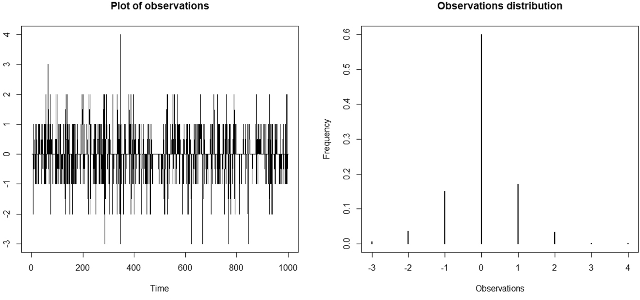
From left to right: plot and distribution of n = 1000 observations simulated from EP-RBINAR(1) process, where actual values are α = 0.45, p = 0.5, and λ = 0.3.
2.2 Properties
The stationarity of the proposed EP-RBINAR(1) process is established in the following theorem.
Theorem 1.
Suppose that
In the sequel, under stationary conditions and using Lemma 1, we derive some properties of the EP-RBINAR(1) process.
Proposition 1.
Let
The probability generating function of the stationary EP-RBINAR(1) process is obtained as
(6)where
and
ρ(1) = corr(X t , X t−1) = 2α − 1
Remark 8.
The stationary conditions associated with the EP-RBINAR(1) process are similar to that of a classical AR(1) process. Indeed, one can see that
where ξ t is a stationary process defined by
Moreover, one can see, based on properties of signed thinning operator that ξ = (ξ t ) is an uncorrelated process. Thus, the EP-RBINAR(1) process has the same autocorrelation structure as a classic AR(1) process. In other words, the autocorrelation function of the EP-RBINAR(1) process is obtained as
Therefore, the spectral density function of the model, for
Under stationary conditions, the marginal probability function of the EP-RBINAR(1) process is given in the following proposition.
Proposition 2.
Let {X
t
} be an EP-RBINAR(1) process, with 0 < α < 1,
where
The EP-RBINAR(1) process’s one-step transition probability, denoted by
and for i ≠ 0
where
Moreover, using the first-order dependence of the process, the joint probability can be obtained as
The k step-ahead conditional mean (usually used for time series forecast issues) of the process is derived in the following proposition.
Proposition 3.
Let {X
t
} be an EP-RBINAR(1) process with 0 < α < 1,
Remark 9.
Using Equation (10), we find that
which is the unconditional mean of the EP-RBINAR(1) process.
3 Parameters Estimation
Let
3.1 Yule–Walker Estimation
Let
In order to obtain estimations in this method, we solve a set of equations that are resulted from equating the theoretical and empirical aspects at the same time. Thus, the YW estimation of α is obtained by
and the YW estimation of p and λ are obtained by solving the following equations
Remark 10.
A special case of our model, when we suppose that α = p. In this case, the YW estimation of α (and p) is
and the YW estimation of λ is given by
3.2 Conditional Least Square Estimation
Let γ = 2α − 1 and μ = (2p − 1)λ, then the CLS estimator of θ* = (γ, μ) is defined by
where
Remark 11.
Based on Theorem 1, we have
The CLS estimation is asymptotically normal.
Remark 12.
A special case of the proposed model, when we suppose that α = p. In this case, the CLS estimation of α (and p) is given as
and the CLS estimation of λ is given by
3.3 Conditional Maximum Likelihood Estimation
From the joint probability function (9), the conditional log-likelihood function for the EP-RBINAR(1) model can be written as
where
The conditional maximum likelihood (CML) estimator
4 Empirical Study
This section includes two subsections. In the first part, the performance of estimation methods that we used for parameters of the proposed process is compared through a simulation study. To ensure the applicability of the proposed model, the second part is devoted to analyzing a practical data set of the Saudi stock market.
4.1 Simulation
4.1.1 The Case When α = p
In this section, we aim to test the efficiency of the parameter’s estimation discussed in the previous section. For the sake of simplicity, we suppose that α = p. Thus, we simulate (using the R programming language) 1000 paths of length 100, 500, 1000 and 10,000. These paths are simulated using Equation (3) with three sets of parameters: (a) α = p = 0.1 and λ = 1; (b) α = p = 0.6 and λ = 2; (c) α = p = 0.9 and λ = 3. Mean values of YW, CLS, and CML estimates for each set of parameters are given in Table 1. The standards deviations of the estimates are stated in brackets under the estimated values.
Estimated parameters and the corresponding standard errors (in brackets) stated under the estimates for YW, CLS and CML methods (when α = p).
| Size |
|
|
|
|
|
|
|
|---|---|---|---|---|---|---|---|
| a) α = p = 0.1 and λ = 1 | |||||||
|
|
|||||||
| n = 100 | 0.110 | 1.009 | 0.109 | 1.010 | 0.101 | 0.977 | |
| (0.034) | (0.176) | (0.034) | (0.175) | (0.028) | (0.120) | ||
| n = 500 | 0.102 | 1.002 | 0.101 | 1.002 | 0.102 | 1.000 | |
| (0.015) | (0.076) | (0.015) | (0.076) | (0.011) | (0.050) | ||
| n = 1000 | 0.101 | 1.002 | 0.101 | 1.002 | 0.099 | 1.006 | |
| (0.010) | (0.054) | (0.010) | (0.054) | (0.009) | (0.041) | ||
| n = 10,000 | 0.100 | 0.999 | 0.100 | 0.999 | 0.0999 | 1.000 | |
|
|
|||||||
| (0.003) | (0.016) | (0.003) | (0.016) | (0.002) | (0.011) | ||
|
|
|||||||
| b) α = p = 0.6 and λ = 2 | |||||||
|
|
|||||||
| n = 100 | 0.592 | 1.584 | 0.592 | 1.513 | 0.593 | 2.019 | |
| (0.050) | (21.931) | (0.050) | (23.147) | (0.033) | (0.172) | ||
| n = 500 | 0.598 | 2.251 | 0.597 | 2.252 | 0.599 | 1.987 | |
| (0.023) | (1.048) | (0.023) | (1.047) | (0.015) | (0.082) | ||
| n = 1000 | 0.599 | 2.101 | 0.599 | 2.101 | 0.597 | 1.999 | |
| (0.016) | (0.660) | (0.016) | (0.659) | (0.011) | (0.061) | ||
| n = 10,000 | 0.599 | 2.004 | 0.599 | 2.005 | 0.598 | 1.999 | |
|
|
|||||||
| (0.005) | (0.184) | (0.005) | (0.184) | (0.004) | (0.052) | ||
|
|
|||||||
| c) α = p = 0.9 and λ = 3 | |||||||
|
|
|||||||
| n = 100 | 0.887 | 3.454 | 0.883 | 3.704 | 0.899 | 2.999 | |
| (0.317) | (1.377) | (0.032) | (1.445) | (0.012) | (0.283) | ||
| n = 500 | 0.897 | 3.100 | 0.896 | 3.152 | 0.899 | 2.996 | |
| (0.013) | (0.535) | (0.136) | (0.544) | (0.005) | (0.129) | ||
| n = 1000 | 0.898 | 3.040 | 0.898 | 3.065 | 0.899 | 3.000 | |
| (0.009) | (0.379) | (0.009) | (0.382) | (0.003) | (0.089) | ||
| n = 10,000 | 0.899 | 3.004 | 0.899 | 3.007 | 0.899 | 3.002 | |
| (0.003) | (0.114) | (0.003) | (0.114) | (0.002) | (0.064) | ||
Remark 13.
In the case when α = p, one can use results presented in Remarks 10 and 12 to calculate YW and CLS estimates. However, CML estimates are calculate by using numerical methods. Explicitly, we use the nlm function (Non-Linear Minimization, from package “stats”, software R), to find values that maximize the conditional log-likelihood function, denoted by (14) (where we consider that α = p in this equation).
In general way, from the obtained results, one can deduce that YW, CLS and CML methods provide estimates that are quite close to the actual values. Moreover, the performances of YW and CLS methods are very similar. For these methods, one can see that when the length of series is over 500, they converge quickly to the actual parameter values. However, results of CML method are more efficient even for a small length of series. For all the proposed methods, we can notice that the standard deviation of the estimates decreases as the length series increases. Furthermore, in most of studied cases, the CLM method provides the lower standard deviation of estimates.
However, for YW and CLS methods, it is important to point the convergence rate is less quickly for λ. Indeed, this can be explained by the fact that, for both methods, the estimate of λ depends on the estimated value of α. Thus, for these methods, we find that a large current value of λ implies the standard deviation of the estimates is high, especially when the size of the series is small. This remark is illustrated thanks to the simulation results obtained for parameters set (c) (for details, see Table 1). The boxplots for the parameter set (c) are given in Figures 2 –4 for CLS, YW and CML methods, respectively. One can see that, contrary to the other methods, the estimates from the CML method have few or no outliers.
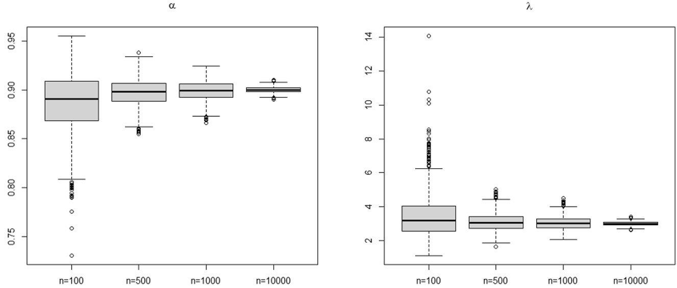
The boxplot for CLS estimates for parameters set (c), where actual values are α = p = 0.9 and λ = 3.
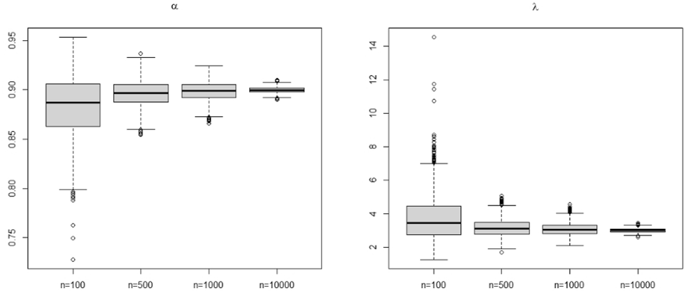
The boxplot for YW estimates for parameters set (c), where actual values are α = p = 0.9 and λ = 3.
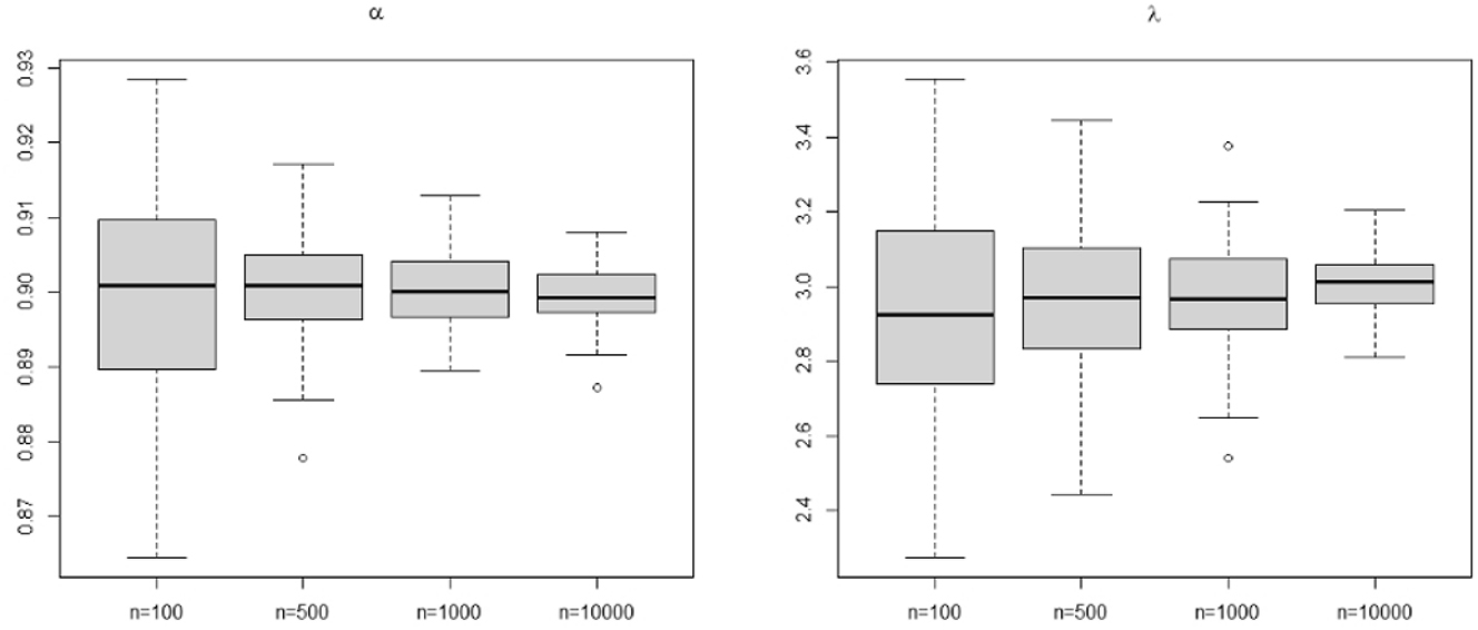
The boxplot for CML estimates for parameters set (c), where actual values are α = p = 0.9 and λ = 3.
On the other hand, one can see, based on the simulation results of YW and CLS methods, obtained for parameter set (b) when n = 100, that the standard deviation of λ estimates is very high for both methods (see Table 1). In fact, these results are not surprising cause that α (= p) actual value is close to 0.5 (which is an excluded value of the parameter). So, with a small size of series the estimate value of α may be close to 0.5, which can “explode” the estimate value of λ. However, this issue is not present when we use the CML method (in this case, even with a small length series, the standard deviation is weak, see Table 1). Finally, fitting to the Gaussian distribution is illustrated in Figures 5 and 6 for YW, CLS and CML estimators (with the parameter set (c) and n = 10,000). These figures show numerically the normal asymptotical distribution of the proposed estimators.
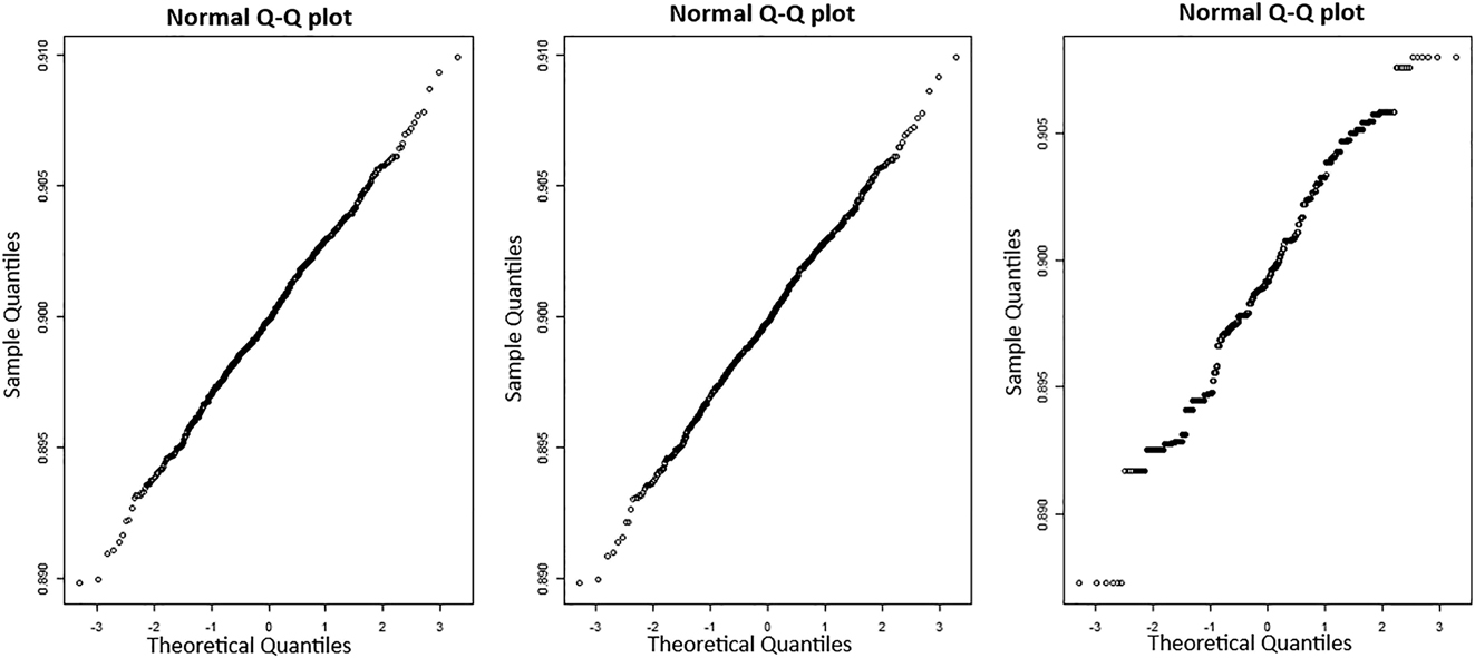
Normal Q-Q plots for errors
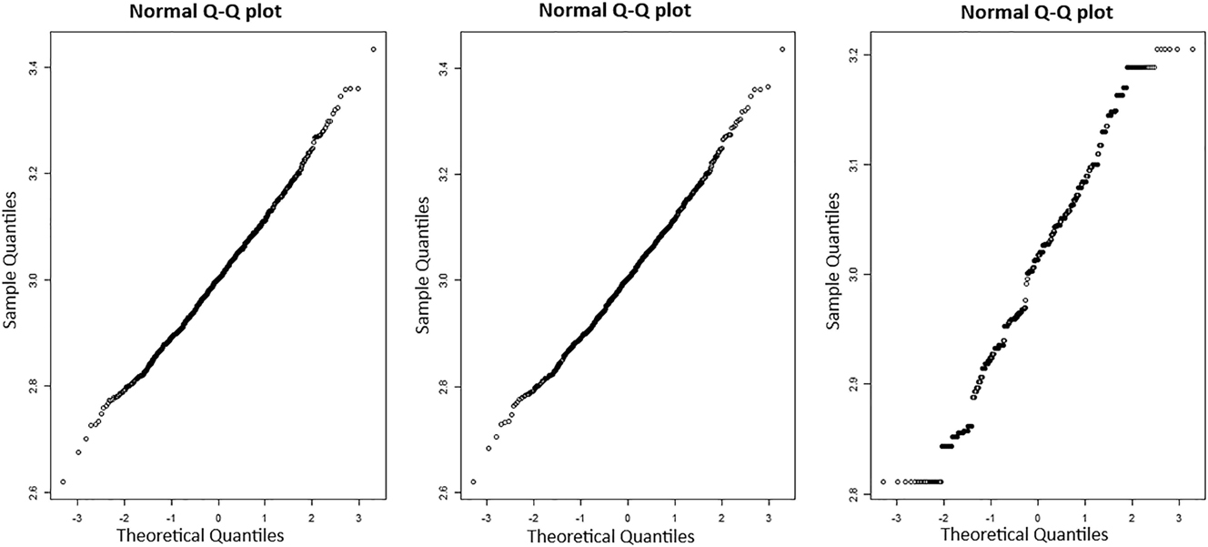
Normal Q-Q plots for errors
4.1.2 The Case When α ≠ p
As we mentioned in the previous section, the performance of the YW and CLS methods are quite close. Moreover, we have also seen that if α ≠ p, then the estimates of these methods do not have an explicit form. Thus, in this section, we will compare the performances resulting from the YW and CML methods based on one set of parameters: α = 0.75, p = 0.4, and λ = 2. We simulate (using the R programming language) 10,000 paths of length 100, 250, and 1000. These paths are simulated using Equation (3) with the above set of parameters. To calculate the CML estimates we use the nlm function (Non-Linear Minimization, from package “stats”, software R) to find values that maximize the conditional log-likelihood function, denoted by (14). On the other hand, the YW estimates of α is given by (11). Once we estimate the value of parameter α (based on (11)) and substitute this value into Equation (12), we get the system of two equations with two unknown variables λ and p. To find YW estimates of these parameters, this system has to be solved numerically. Thus, the numerical procedure will be conducted in programming language R, where we will use the BB package. Mean values of YW and CML estimates for each parameters are given in Table 2. The standards deviations of the estimates are stated in brackets under the estimated values. Once again, we can see that the precision of these estimates (from both methods) increases when the size n increases.
Estimated parameters and the corresponding standard errors stated (in brackets) under the estimates for YW and CML methods (when α ≠ p).
| α = 0.75, λ = 2, and p = 0.4 | ||||||
|---|---|---|---|---|---|---|
| Size |
|
|
|
|
|
|
| n = 100 | 0.739 | 1.981 | 0.389 | 0.739 | 1.997 | 0.397 |
| (0.046) | (0.186) | (0.074) | (0.078) | (0.171) | (0.065) | |
| n = 250 | 0.748 | 1.982 | 0.412 | 0.746 | 2.012 | 0.402 |
| (0.015) | (0.129) | (0.045) | (0.069) | (0.103) | (0.039) | |
| n = 1000 | 0.749 | 2.002 | 0.401 | 0.749 | 1.999 | 0.399 |
| (0.015) | (0.054) | (0.019) | (0.019) | (0.052) | (0.019) | |
Remark 14.
In order to study the compatibility of the proposed model and the estimation results, we generated, based on Equation (1), n = 1000 observations of the EP-RBINAR(1) process, with α = 0.75, p = 0.4, and λ = 2. Basic descriptive statistics associated with the simulated data are represented in the following table:
| Indicator | Mean | Variance | First autocorrelation | Second autocorrelation | Third autocorrelation |
|---|---|---|---|---|---|
| Empirical value | −0.936 | 8.590494 | 0.48065090 | 0.20075170 | 0.06104609 |
Using the simulated data and the procedure presented in the above section, we compute the CML estimates of the process parameters:
| Indicator | Mean | Variance | First autocorrelation | Second autocorrelation | Third autocorrelation |
|---|---|---|---|---|---|
| Estimate value | −0.8694537 | 8.487022 | 0.48622 | 0.2364099 | 0.1149472 |
Thus, one can see that empirical values of these indicators are very close to that of estimate values (calculated based on estimate parameters and properties of the process).
4.2 A Practical Data Example
Here, we present an application of the model EP-RBINAR(1) based on real-world data from Saudi stock market. In 2007, the minimum amount of change was 0.25 SR (Saudi Riyal) for all stocks. The daily close price as number of ticks (ticks = close price × 4) in 2007 for Saudi Telecommunication Company (STC) stock is considered. Note that these data were originally introduced by Alzaid and Omair (2014) as an application of a new integer-valued model with a Poisson difference marginal distribution. This model can be used as a tool to model non-stationary count data. Basic descriptive statistics concerning these data are presented in Table 3.
Basic descriptive statistics for the STC stock data set.
| Length | Mean | Minimum | Maximum | First quartile | Median | Third quartile | Standard deviation |
|---|---|---|---|---|---|---|---|
| 248 | 49.82 | 45 | 66 | 46 | 48 | 52 | 4.6968 |
After, examination of the time series plot of the data, authors (Alzaid and Omair (2014)) notice a non-stationarity in the mean (this issue was confirmed based on a sustained large autocorrelation function (ACF) and exceptionally large first lag partial autocorrelation function (PACF)). Thus, authors considered that differencing is needed. Explicitly, if {X t } is the process behind the above data, then authors propose to study the lag one differenced process, denoted by {Y t }, where Y t = X t − X t−1. Indeed, one can consider that data observed from process {Y t } as the difference between two consecutive daily ticks (associated with the close price). Thus, a data with negative values represents the number of ticks “lost” at the close between two consecutive days (i.e. a drop in price), while a positive value reveals the number of ticks “gained” at the close between two consecutive days (i.e. a price increase). Finally, if the observed data is zero, this means that the number of ticks at closing has remained “stable” between two consecutive days (i.e. the price has not changed).
The time series plot of the differenced stock is illustrated in Figure 7 and basic descriptive statistics concerning the differenced data are presented in Table 4. Thus, Figure 7 shows the stationarity in the mean is now verified. The ACF and PACF for differenced stock are shown in Figure 8. These figures show that the lag one correlation is positive and significant, which implies that the differenced process have the same autocorrelation structure of an AR(1) process. Moreover, after the lag one differenced stage, the data is integer with negative values.
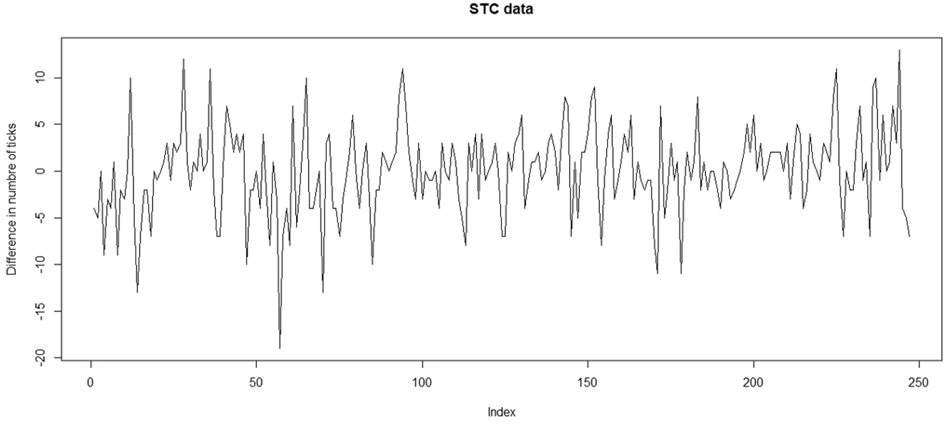
The time series plot of the differenced STC stock data set.
Basic descriptive statistics for the differenced STC data set.
| Length | Mean | Minimum | Maximum | First quartile | Median | Third quartile | Standard deviation |
|---|---|---|---|---|---|---|---|
| 247 | 0.004049 | −19 | 13 | −2 | 0 | 3 | 4.715049 |
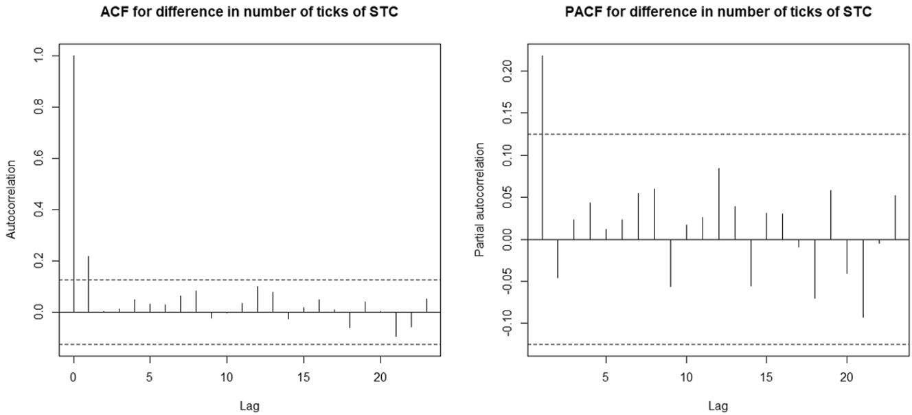
The ACF and PACF of the differenced STC stock data set.
Remark 15.
Bourguignon and Vasconcellos (2016) have used data, dating from 2012, providing also from Saudi Telekom. The choice of these data is consistent with the model proposed by the authors (where they introduced a new process (defined on
To fit the differenced data, we propose our EP-RBINAR(1) process. Explicitly, we consider that
where F is as defined in (2) and ϵ
t
follows an E-Po(p, λ), where 0 < p < 1, λ > 0 and
Remark 16.
Based on properties of the process and using the estimates of the unknown parameters, one can deduce that the mean is equal to 0.3311299 (which is not close enough to 0.004048583 (mean of the data) however, one can consider that both values are near to zero), the standard deviation equals 4.246681 (which is close to 4.715049, the standard deviation calculated from the data), and the lag-1 autocorrelation is equal to 0.289729 (which is close to 0.2194211, lag-1 autocorrelation calculated from the data). These first results support our choice of the EP-RBINAR(1) model to fit the data.
Moreover, based on the conditional one-step ahead mean, the estimated residuals are computed as
Remark 17.
In general,
To verify the adequacy of the considered model, the ACF and the PACF of the estimated residuals are plotted in Figure 9. Clearly, this graph shows that the residuals can be considered as observations from a white noise. Moreover, in Figure 10, we make a comparison between the empirical frequencies of
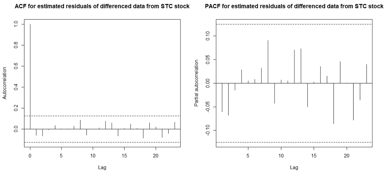
The ACF and PACF of the estimated residuals of the differenced STC stock data set.
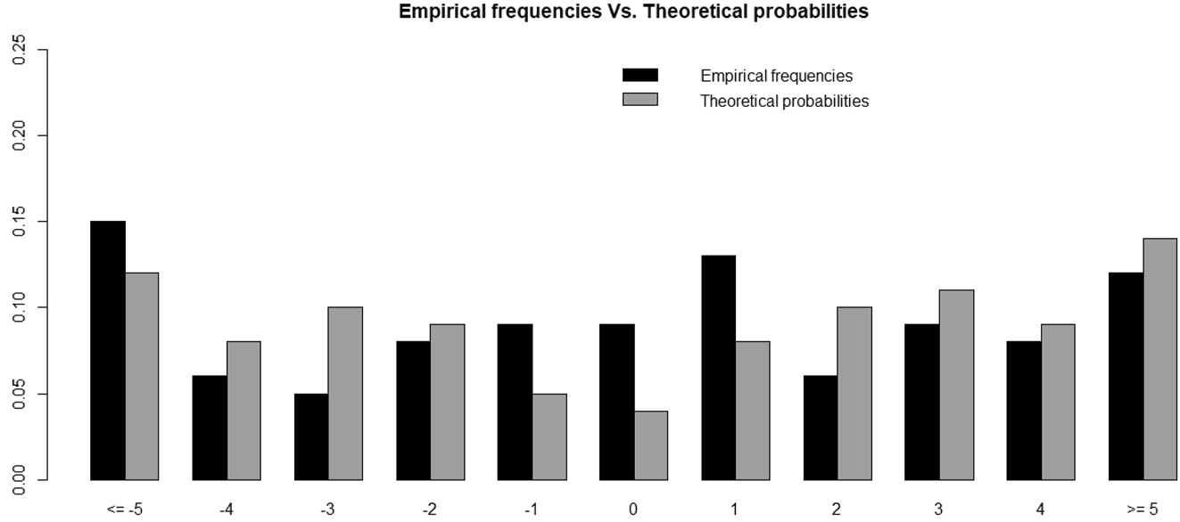
Comparison between the empirical frequencies of estimated residuals and their associated theoretical probabilities resulting from E-Po(0.5345621, 3.402455).
Remark 18.
Based on the conditional one-step ahead standard deviation, the estimated standardized Pearson residuals are computed as
For details concerning the standardized Pearson residuals and its role to check model adequacy for count time series, see Weiß et al. (2019). Note that the empirical mean, median, and standard deviation, of the estimated standardized Pearson residuals, are, respectively, equals: −0.05694, 0, and 1.127245. Thus, one can see that the empirical mean is very close to zero and empirical standard deviation is close to one. Moreover, the ACF, the PACF, and the fitting to the Gaussian distribution (Normal Q-Q plot) of the estimated standardized Pearson residuals are plotted in Figure 11. These results can be considered as additional arguments whose objective is to check the model adequacy to fit the data.
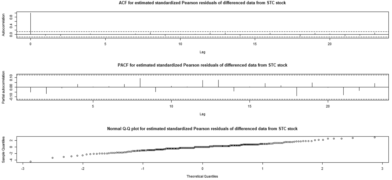
From top to bottom: ACF, PACF, and normal Q-Q plot of estimated standardized Pearson residuals of the differenced STC stock data set.
Remark 19.
As mentioned before, the data processed in this section have been studied by Alzaid and Omair (2014). Indeed, authors proposed their model, called PDINAR(1) process, to fit the data. However, this process has two variants, denoted by PDINAR+ (1) and PDINAR− (1), depending on the sign of the correlation. In practice, to fix which variant should be used to fit the data, it is necessary to have a preliminary idea of the sign of
These predicted values need also to by rounding to the nearest integer to be adequate with the discrete support of the data. From Figure 12, one can deduce that the predictions (based on conditional one-step ahead mean) results provided from PDINAR+ (1) process and those from the EP-RBINAR(1) process, are very similar. This implies that both models have a prediction performances very close. Indeed, the Root Mean Squared Error (RMSE) equals 4.604699 (resp. 4.590552), for forecasting values (based on conditional mean) provided from PDINAR+ (1) (resp. EP-RBINAR(1)) process. However, one can see also that for both models there is a rather discrepancy between the forecast and the actual data.
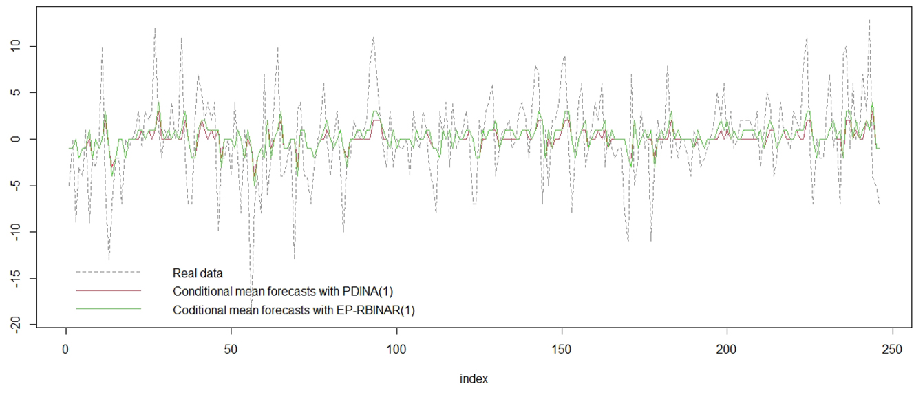
Comparison of conditional mean predictions results from PDINAR(1) and EP-RBINAR(1).
Remark 20.
As mentioned above, conditional one-step ahead mean leads to real-valued forecasts, which is incoherent with the support of the integer-valued time series. Recently, coherent techniques have been introduced in order to provide integer-valued forecasts. One of the most used technique is the conditional median (for details, see Homburg et al. (2019)), which is obtained by calculating the conditional probability of each possible integer value, then selecting a forecast value with a cumulative conditional probability greater than 0.5. From Figure 13, one can see that discrepancy between conditional median forecasts and actual data have been reduced, specially for high positive values. Moreover, one can find that the Mean Absolute Error (MAE) (based on the conditional median forecasts) equals 3.768293 and Median Absolute Error (MedAE) equals 3.
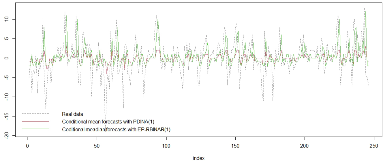
Comparison between conditional mean predictions results of PDINAR(1) and conditional median predictions of EP-RBINAR(1).
5 Concluding Remarks
In this paper, we introduce a new stationary first-order integer-valued autoregressive process, denoted by EP-RBINAR(1), where the thinning part of the process can be considered as the sum of a random walk. The new model has several advantages: possible negative values for time series, possible negative values for autocorrelation, and an innovation structure that can be interpreted as an extension on
Proof of Lemma 1. In proving all cases, we use this fact that
For any
where
where Z ∼ B(2|x|, α) and sign(x)|x| = x. So, we have
First note that
By utilizing the fact that max(|a| − |b|, 0) ≤ |a − b| ≤ |a| + |b|, we obtain
the proof is completed by substituting
Proof of Theorem 1. Under the assumptions of Theorem 1, one can deduce that
The root of the polynomial function
is outside the unit disc (i.e.
Consequently, assumptions of Theorem 1 of Kachour and Truquet (2011) are verified. Thus, one can confirm that the process X t defined in (3) has a unique stationary solution. In other hand, from Remarks 2 and 5, for all positive integer l > 2, we have that
The lth moment of F is finite,
Once again, based on Theorem 1 of Kachour and Truquet (2011), one can deduce that
Proof of Proposition 1. Let
□
Proof of Proposition 2. Note that, for all
where
Now, by substituting (16) into (15), we have
where
The proof is completed. □
Proof of Proposition 3. Using Proposition 1, the one step-ahead conditional mean equals
Based on the above equation, we have
and in the same manner, one can see that
Hence by induction, one can conclude that
□
References
Al-Osh, M. and Alzaid, A.A. (1987). First-order integer-valued autoregressive (INAR(1)) process. J. Time Ser. Anal. 8: 261–275, https://doi.org/10.1111/j.1467-9892.1987.tb00438.x.Search in Google Scholar
Alzaid, A.A. and Omair, M.A. (2014). Poisson difference integer valued autoregressive model of order one. Bull. Malaysian Math. Sci. Soc. 37: 465–485.Search in Google Scholar
Bakouch, H.S., Kachour, M., and Nadarajah, S. (2016). An extended Poisson distribution. Commun. Stat. Theor. Methods 45: 6746–6764, https://doi.org/10.1080/03610926.2014.967587.Search in Google Scholar
Barreto-Souza, W. and Bourguignon, M. (2015). A skew INAR(1) process on Z. AStA Adv. Stat. Anal. 99: 189–208, https://doi.org/10.1007/s10182-014-0236-2.Search in Google Scholar
Bourguignon, M. and Vasconcellos, K.L. (2016). A new skew integer valued time series process. Stat. Methodol. 31: 8–19, https://doi.org/10.1016/j.stamet.2016.01.002.Search in Google Scholar
Bulla, J., Chesneau, C., and Kachour, M. (2011). A bivariate first-order signed integer-valued autoregressive process. Commun. Stat. Theory Methods 46: 6590–6604.10.1080/03610926.2015.1132322Search in Google Scholar
Chen, H., Zhu, F., and Liu, X. (2023). Two-step conditional least squares estimation for the bivariate Z-valued INAR(1) model with bivariate Skellam innovations. Commun. Stat. Theor. Methods, https://doi.org/10.1080/03610926.2023.2172587.Search in Google Scholar
Chesneau, C. and Kachour, M. (2012). A parametric study for the first-order signed integer-valued autoregressive process. J. Stat. Theory Pract. 6: 760–782, https://doi.org/10.1080/15598608.2012.719816.Search in Google Scholar
Freeland, R.K. (2010). True integer value time series. AStA Adv. Stat. Anal. 94: 217–229, https://doi.org/10.1007/s10182-010-0135-0.Search in Google Scholar
Homburg, A., Weiß, C.H., Alwan, L.C., Frahm, G., and Göb, R. (2019). Evaluating approximate point forecasting of count processes. Econometrics 7: 30, https://doi.org/10.3390/econometrics7030030.Search in Google Scholar
Kachour, M. (2014). On the rounded integer-valued autoregressive process. Commun. Stat. Theor. Methods 43: 355–376, https://doi.org/10.1080/03610926.2012.661506.Search in Google Scholar
Kachour, M. and Truquet, L. (2011). A p-order signed integer-valued autoregressive (SINAR(p)) model. J. Time Ser. Anal. 32: 223–236, https://doi.org/10.1111/j.1467-9892.2010.00694.x.Search in Google Scholar
Kachour, M. and Yao, J.F. (2009). First-order rounded integer-valued autoregressive (RINAR (1)) process. J. Time Ser. Anal. 30: 417–448, https://doi.org/10.1111/j.1467-9892.2009.00620.x.Search in Google Scholar
Kim, H.Y. and Park, Y. (2008). A non-stationary integer-valued autoregressive model. Stat. Pap. 49: 485–502, https://doi.org/10.1007/s00362-006-0028-1.Search in Google Scholar
Latour, A. and Truquet, L. (2008). An integer-valued bilinear type model, Available at: http://hal.archives-ouvertes.fr/hal-00373409/fr/.Search in Google Scholar
Liu, Z., Li, Q., and Zhu, F. (2021). Semiparametric integer-valued autoregressive models on. Can. J. Stat. 49: 1317–1337, https://doi.org/10.1002/cjs.11621.Search in Google Scholar
McKenzie, E. (1985). Some simple models for discrete variate time series. Water Resour. Bull. 21: 645–650, https://doi.org/10.1111/j.1752-1688.1985.tb05379.x.Search in Google Scholar
Scotto, M.G., Weiß, C.H., and Gouveia, S. (2015). Thinning-based models in the analysis of integer-valued time series: a review. Stat. Model. Int. J. 15: 590–618, https://doi.org/10.1177/1471082x15584701.Search in Google Scholar
Steutel, F.W. and van Harn, K. (1979). Discrete analogues of self-decomposability and stability. Ann. Probab. 7: 893–899, https://doi.org/10.1214/aop/1176994950.Search in Google Scholar
Taveira da Cunha, E., Vasconcellos, K.L., and Bourguignon, M. (2018). A skew integer-valued time-series process with generalized Poisson difference marginal distribution. J. Stat. Theory Pract. 12: 718–743, https://doi.org/10.1080/15598608.2018.1470046.Search in Google Scholar
Weiß, C.H. (2008). Thinning operations for modeling time series of counts-a survey. AStA Adv. Stat. Anal. 92: 319–343.10.1007/s10182-008-0072-3Search in Google Scholar
Weiß, C., Scherer, L., Aleksandrov, B., and Feld, M. (2019). Checking model adequacy for count time series by using Pearson residuals. J. Time Econom. 12: 2018–0018.10.1515/jtse-2018-0018Search in Google Scholar
Zhang, H., Wang, D., and Zhu, F. (2010). Inference for INAR (p) processes with signed generalized power series thinning operator. J. Stat. Plann. Inference 140: 667–683, https://doi.org/10.1016/j.jspi.2009.08.012.Search in Google Scholar
Zhang, H., Wang, D., and Zhu, F. (2012). Generalized RCINAR (1) process with signed thinning operator. Commun. Stat. Theor. Methods 41: 1750–1770, https://doi.org/10.1080/03610926.2010.551452.Search in Google Scholar
© 2023 the author(s), published by De Gruyter, Berlin/Boston
This work is licensed under the Creative Commons Attribution 4.0 International License.
Articles in the same Issue
- Frontmatter
- Editorial
- Editorial Announcement
- Original Articles
- A New INAR(1) Model for ℤ-Valued Time Series Using the Relative Binomial Thinning Operator
- Is a Secondary Currency Essential? – On the Welfare Effects of a New Currency
- Data Observer
- Beyond the Business Climate: Supplementary Questions in the ifo Business Survey
- Identifying Supervisory or Managerial Status in German Administrative Records