Employing variance component estimation for point cloud based geometric surface representation by B-splines

2.1 Surface representation using TP B-splines

In surface modeling based on point clouds the usage of B-splines allows deriving a statement on (significant) present deformation between consecutively acquired data of an object of interest [7], 9]. A TP B-spline surface is defined as follows:

It can be regarded as the composition of an infinite number of B-spline curves running in two different parameter directions u and v. One point S(u, v) on the surface is determined as the weighted sum of the control points P_i,j. The weights are recursively formulated Bernstein polynomials, whose occurrence or elimination depend on the knot vectors U resp. V and the respective degrees p and q [14], p. 50]. The net of the control points P_i,j builds the scaffold of the surface. A geometrical change of a point on the surface is linked to a change within the set of connected control points.

2.2 Incorporation of the stochastic model in the surface representation

The approximation of a point cloud by a TP B-spline surface can be formulated in a GMM, where the observations l are the points' cartesian coordinate elements. The design matrix A incorporates the partial derivations of the respective functional model according to the unknowns. An enhancement by the stochastic model in the form of a dispersion matrix Σ _ll is feasible [15]. For the incorporation of the surface approximation formulated in a GMM in a VCE, the observations must not contain any outliers. An approach for robust estimation of B-spline surface parameters is examined in [16]. As this paper is based on simulated data, no outliers are comprised in the data.

2.3 VCM comprising measurement uncertainties

The measurement uncertainties impact the noise level of each individual point of a point cloud. The uncertainties concerning the range and angular measurement are typically stated by the manufacturer. The establishment of a VCM incorporating these uncertainties is obtained by error propagation (EP). The functional relation between a point cloud in 3D cartesian space and the measured geometric elements are:

wherein [x,y,z]^⊺ are the cartesian coordinate elements of one point, r is the measured distance, hz the measured horizontal direction and v the vertical angle. By applying EP, the VCM Σ _ll ^meas of the point cloud’s coordinate elements is set up. In the context of VCE, the VC of the measurement elements r, hz and v shall be estimated. The overlap of the components is outlined in the following with reduction of the equation (2) into 2D space for the sake of easier legibility. The transfer onto equation (2) can be extended straightforward.

2.4 Deriving empirical VCM from given data

To address the stochastic representation of residual systematics, an empirical VCM of a point cloud relative to a geometric model S(u, v) can be constructed using covariance functions.

The residuals are given as deviations

representing the variability of the point cloud in respect to the model S(u, v). In order to compactly summarize the variability of the points deviations δ, empirical autocovariance functions C ̂ x x ( d ̄ k ) , C ̂ y y ( d ̄ k ) and C ̂ z z ( d ̄ k ) as well as crosscovariance functions C ̂ x y ( d ̄ k ) , C ̂ x z ( d ̄ k ) and C ̂ y z ( d ̄ k ) are estimated as exemplarily shown for C ̂ x y ( d ̄ k ) in equation (6) [17], p. 341ff]:

This computation requires a subdivision of the data points’ separation distances d _ij = ‖S(u _i , v _i ) − S(u _j , v _j )‖ into consecutive intervals N _k of size |N _k |, each with a mean separation distance d ̄ k , as the data points are not equidistant. The chosen approach is similar to the estimation of variogrammes and covariogrammes in the case of collocation [18], p. 131]. In order to ensure a stable estimation, only data pairs with a spatial distance less than or equal half of the diameter of the entire region covered by the incorporated points are taken into account [19], p. 32].

Having estimated the empirical covariance functions, analytical positive semidefinite functions C x x ( d ̄ k ) , … , C y z ( d ̄ k ) are used to approximate the empirical values and to guarantee positive semidefinite covariance matrices. The covariance matrices are set up by means of the analytical functions as follows:

with the autocovariance Σ _ii and crosscovariance matrices Σ _ij being established as follows:

2.5 Estimation of VC using a best invariant quadratic unbiased estimation (BIQUE)

Alongside the assessment of unknown parameters in a GMM, whose functional model is expressed by (1), the estimation of VC α _i comprised in the VCM Σ _ll of the observations – being the point cloud – is feasible, provided that a parametrized stochastic model is implemented [15], p. 227ff]:

The parameter α i 2 is the factor of the variance resp. covariance to be estimated. The parameter m is the number of (co-)variance components that are assessed and accordingly, the number of splitted covariance matrices that form the overall VCM of the observations l [15], p. 227ff].

The estimation of VC is a generalization of the assessment of the variance of the unit weight s 0 2 = v ⊺ P v n f where P = Σ l l − 1 . Likewise to the estimation of the unknowns in the GMM, the determination of the VC follows a best unbiased estimation given that

The expectancy value E of the quadratic sum of the observations weighted by the estimator matrix D is set equal to the scalar form p^⊺ ⋅ α, whereas α = α 1 1 , α 2 2 , … , α m 2 ⊺ is the vector of estimated VC and p is used as vector with logical entries indicating the estimation of one specific variance component α i 2 . Given the added condition that the estimation minimizes the variance

[20] introduces VCE using a BIQUE approach. For this, an additional constraint must be satisfied, requiring the invariance of the VC α w.r.t. the unknown parameters. This constraint is expressed as D ⋅ A = 0 and p _i = tr(D ⋅ Σ _i ), where A is the design matrix setup in the GMM.

By derivation of equation (9) and imposing the additional condition (10) and the constraint on independence from the parameter space, one obtains according to [20]

The estimation of the VC is retrieved by

The VC are estimated iteratively. The starting values for all α i 2 are set to 1. The determination of the VC α ̂ is local which means it is a prerequisite that the factors α i 2 are near 1 in order to achieve convergence in an iterative estimation process [15], p. 227ff].

3.1 Conceptional considerations

As a first step towards the application of the VCE in the context of B-spline surface approximation, simulation studies are conducted. In Figure 1 the steps of the setup of the study are displayed.

Figure 1:

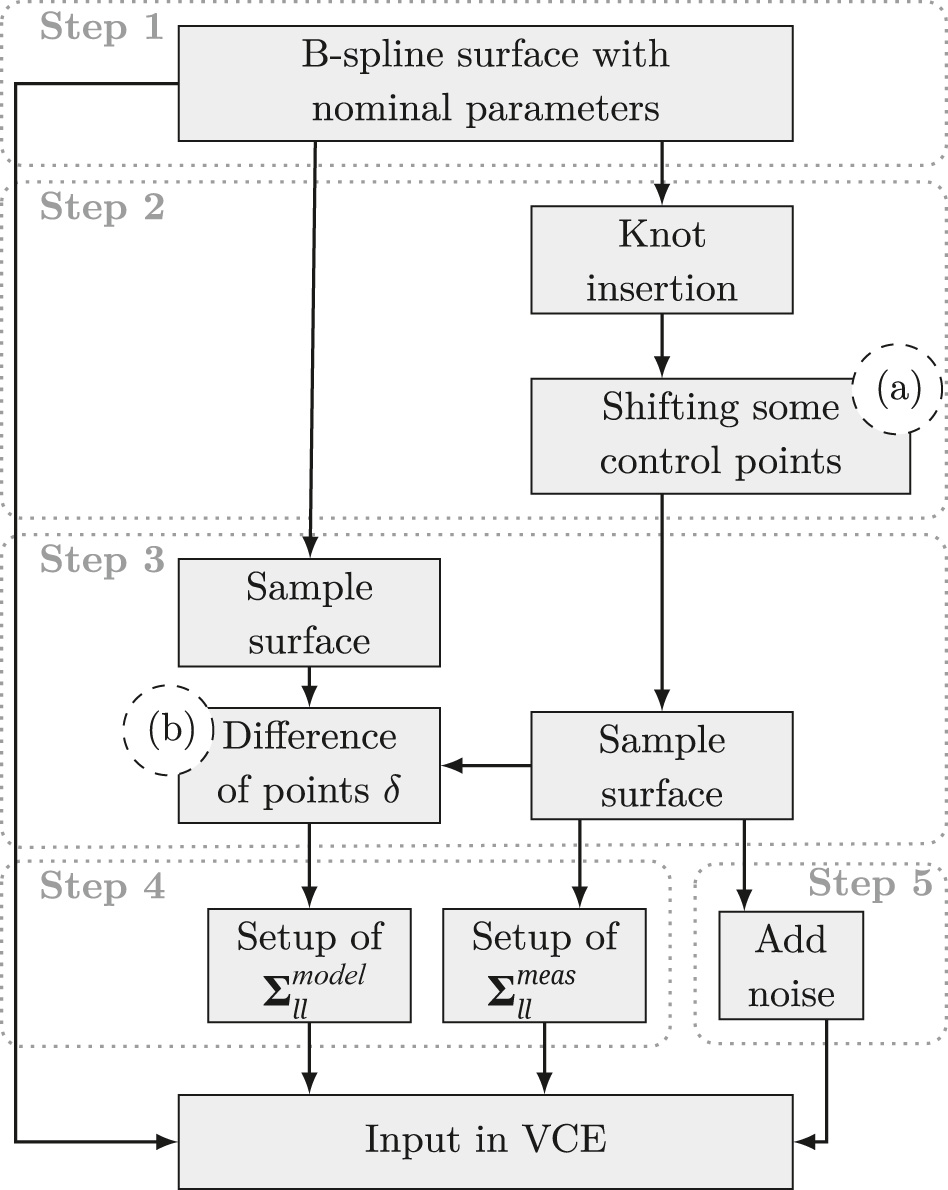
Workflow for the setup of the simulation study. Indicators (a) and (b) refer to Figure 2. The respective steps are discussed in detail in Sections 3.1 and 3.2.

A TP B-spline surface of well-known shape and parameters is used as geometrical (functional) model (Figure 1, Step 1). In the following this surface will be referred to as initial surface S₁(u, v). On basis of this surface, the simulation of the model uncertainty is conducted.

The model uncertainty is considered as the deviation that occurs when the chosen complexity of the functional model, used in the surface approximation, does not adequately reflect the geometric details contained in the point cloud. For TP B-splines, complexity refers to the number of control points.

The deviation of a point cloud to the model S₁(u, v) is realised by increasing it’s complexity without changing it’s course. This is done by knot resp. control point insertion in selected locations [14], p. 141ff] (Figure 1, Step 2). In a next step, a part of the inserted control points P i , j sel are shifted in the direction of the line-of-sight r ̂ from a specified instrument center X _ST . The amount of displacement of the altered control points P i , j altered is scaled by a respectively randomized value ϵ i , j sel ∼ N (0,1) multiplied by the magnitude factor m _f .

The resulting manipulated surface is referred to as adapted surface S₂(u, v). By sampling both surfaces with identical parameter spacing and location, two point clouds are generated that provide a point-to-point relation ( S 1 ( u i , v i ) = ∧ S 2 ( u i , v i ) ) (Figure 1, Step 3). The derived point pairs’ differences are treated as the residuals to the initial surface as δ = S₁(u, v) − S₂(u, v). Following the setup stated in Section 2.4, the VCM Σ _ll ^model is established covering the model uncertainty (Figure 1, Step 4). As the estimation’s stability of the covariance functions depends on the spatial distance of the used points put in one interval N _k , the spatial extent of the introduced surface deviations is locally restricted w.r.t. the course of the point cloud. Moreover, for the determination of the model uncertainty, only the point correspondences with δ _i > θ, exceeding the other (subsequently) integrated error sources indicated by a threshold θ, are taken into account. For the generation of the VCM covering the measurement uncertainty, the sampled points of the adapted surface S₂(u, v) are transformed in spherical coordinates with respect to the simulated instrument center X _ST . Chosen variances of the spherical coordinate components are re-transformed to cartesian coordinates by EP, obtaining the VCM Σ ^meas _ll (Figure 1, Step 4). The sampled points were perturbed by adding noise with predefined variances different to those chosen in the EP (Figure 1, Step 5). If the variances of the applied noise are equal to those introduced in the EP, the estimation of the VC would resolve immediately. The difference of the chosen variances enable the investigation of the convergence behaviour of the iterative estimation.

The subsequent VCE is performed by incorporating the sampled and perturbed point cloud of S₂(u, v), the joint VCM Σ _ll = Σ _ll ^meas + Σ _ll ^model and the functional model of the initial surface S₁(u, v).

3.2 Numerical setup

The simulation study is realised on the basis of a TP B-spline surface representing the course of a water dam being the test specimen of the research conducted within the project TLS-Defo. The initial surface S₁(u, v) is parametrized by 30 × 10 (u × v) control points and is of degree p, q = 3 (Figure 1, Step 1). The adapted surface S₂(u, v) is generated by knot resp. control point insertion (Figure 1. Step 2). The sampled point clouds comprise 3,000 single points evenly spread over the course of the surfaces (Figure 1, Step 3). For the setup of Σ _ll , the noise levels of the measurement elements are chosen as σ _r = 1 mm and σ_hz,v = 0.3 mgon (Figure 1, Step 4). The standard deviations introduced in the EP for the setup of Σ ^meas _ll differ from the applied standard deviations with σ _r = 2 mm and σ_hz,v = 1 mgon (Figure 1, Step 5).

For the specification of model uncertainty, the location of the inserted and altered control points as well as the magnitude factor m _f of the displacement is varied. An example of one realisation is shown in Figure 2.

Figure 2:

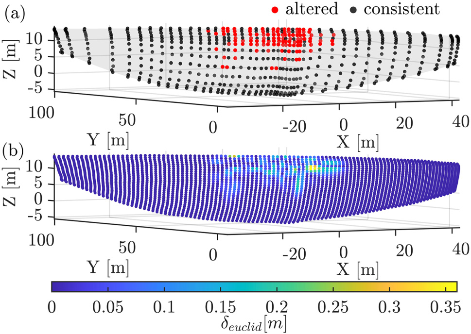
Visualisation of indicators in Figure 1: (a) B-spline surface with control points; (b) sampled points colored by differences δ.

4.1 Monte-Carlo simulation of the measurement uncertainties

To generate a representative result of the simulation study, a Monte-Carlo Simulation (MCS) with multiple realisations of the measurement noise was conducted. In total 600 runs of the VCE were assessed, whereas in each run i an independent setup of the measurement noise was realised by

where ϵ _r , ϵ _hz , ϵ _v ∼ N (0,1) are independent random variables drawn from a standard normal distribution. The VCM of the model uncertainty Σ _ll ^model was fixed for all runs and was built upon the differences of the sampled surface points of the initial and adapted surface. However, solely points with coordinate-wise differences |δ _x | > θ or |δ _y | > θ with θ = 4 mm are used. The specification of the threshold value θ was justified by being twice the magnitude of the mean standard deviation of the lateral components of the perturbed point cloud. Based on the totality of all results of the computed VCE, the mean value and the standard deviation of the estimated variance factors α _i could be determined and are stated in Table 1. For better interpretability, the VC are multiplied with the initially applied variances inserted in the VCM and transformed into standard deviations. They are opposed to the reference values, being the factors of standard deviations that were initially applied to the data.

4.2 Influence of the magnitude of surface deviations on the estimated VC

The setup of the VCM Σ _ll ^model covering the model uncertainty is influenced by two driving factors. Firstly, the location of the displaced control points forming separated regions of deviations. Secondly, the magnitude of the displacements expressed as the magnitude factor in equation (15). This section focuses on the second aspect whilst the first is addressed in the Annex.

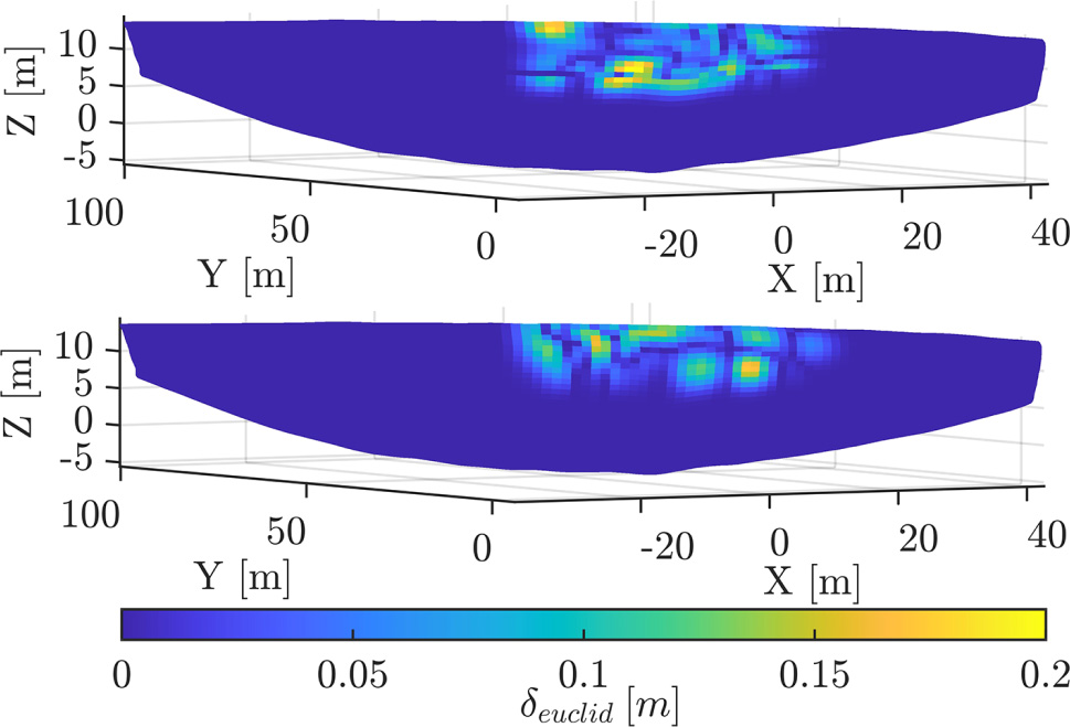
In Figure 3 the displacement between S ₁(u, v) and S ₂(u, v) is shown for two realisations. The pattern of the displacement is consistent. For both cases the selection of the altered control points and the respectively randomized value ϵ are fixed. Solely the magnitude factor m _f is different. To investigate the impact of the magnitude factor m _f on the estimated VC, 11 realisations of the surface deviations are created in reference to the deviation pattern in Figure 3. Herein, m _f ranged from 0.01 to 0.2 m. If the magnitude of displacement is in the range of the propagated measurement uncertainty, affecting the whole point cloud, the separation between model and measurement uncertainty aggravates. This behaviour is displayed in Figure 4.

Figure 3:

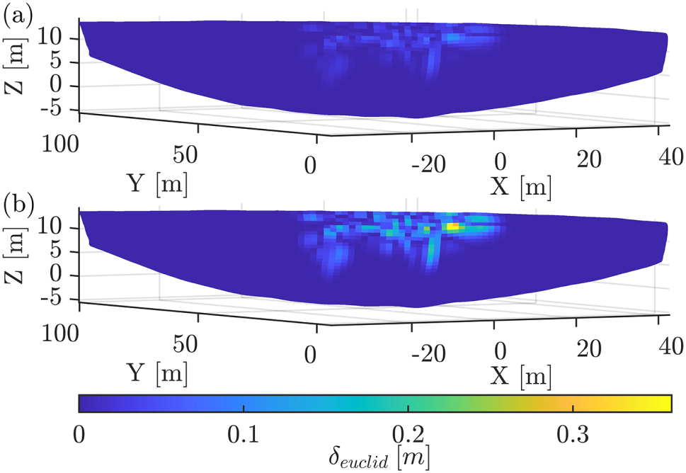
Surfaces colored by δ based on (15) with (a) m _f = 0.06 m, (b) m _f = 0.2 m.

Figure 4:

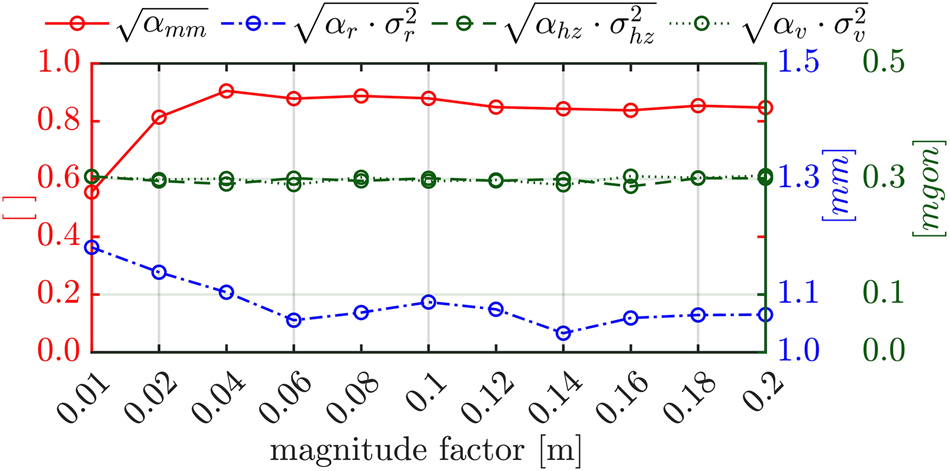
Course of the estimated VC related to a variation of m _f of a fixed selection of control points and a consistent pattern of displacement.

On the abscissa, the magnitude factor for the displacement of a set of control points is plotted. On the ordinate the derived standard deviations impacted by the estimated VC are displayed. The displacement of the control points are performed in the line-of-sight of the simulated scanner position. Hence, it impacts mainly the variance component related to the distance component (blue/dot-dashed) and the model uncertainty (red/solid). The VC related to the angular measurement elements are consistent throughout all estimations (green/dashed resp. dotted). The integrated model uncertainty is intended to be fully depicted in the VCM Σ _ll ^model . Hence, the expected variance component is 1. However, the estimated variance component changes with the variation of m _f . The course of the value change reaches saturation at σ _mm = 0.8 − 0.85.

References

1. Soudarissanane, S, Lindenbergh, R, Menenti, M, Teunissen, P. Scanning geometry: influencing factor on the quality of terrestrial laser scanning points. ISPRS J Photogrammetry Remote Sens 2011;66:389–99. https://doi.org/10.1016/j.isprsjprs.2011.01.005.Suche in Google Scholar
2. International Organization for Standardization. Guide to the expression of uncertainty in measurement. Geneva: International Organization for Standardization; 2008.Suche in Google Scholar
3. Kerekes, G. An elementary error model for terrestrial laser scanning [Dissertation]. Universität Stuttgart; 2023.Suche in Google Scholar
4. Kauker, S, Schwieger, V. A synthetic covariance matrix for monitoring by terrestrial laser scanning. J Appl Geodesy 2017;11:77–87. https://doi.org/10.1515/jag-2016-0026.Suche in Google Scholar
5. Wujanz, D, Burger, M, Tschirschwitz, F, Nietzschmann, T, Neitzel, F, Kersten, TP. Determination of intensity-based stochastic models for terrestrial laser scanners utilising 3d-point clouds. Sensors 2018;18:2187. https://doi.org/10.3390/s18072187.Suche in Google Scholar PubMed PubMed Central
6. Winiwarter, L, Anders, K, Höfle, B. M3C2-EP: pushing the limits of 3d topographic point cloud change detection by error propagation. ISPRS J Photogrammetry Remote Sens 2021;178:240–58. https://doi.org/10.1016/j.isprsjprs.2021.06.011.Suche in Google Scholar
7. Harmening, C. Spatio-temporal deformation analysis using enhanced B-spline models of laser scanning point clouds [Dissertation]. Technische Universität Wien; 2020.Suche in Google Scholar
8. Kerekes, G, Schwieger, V. Elementary error model applied to terrestrial laser scanning measurements: study case arch dam kops. Mathematics 2020;8:593. https://doi.org/10.3390/math8040593.Suche in Google Scholar
9. Kermarrec, G, Kargoll, B, Alkhatib, H. Deformation analysis using b-spline surface with correlated terrestrial laser scanner observations – a bridge under load. Remote Sens 2020;12:829. https://doi.org/10.3390/rs12050829.Suche in Google Scholar
10. Ötsch, E, Harmening, C, Neuner, H. Investigation of space-continuous deformation from point clouds of structured surfaces. J Appl Geodesy 2023;17:151–60.10.1515/jag-2022-0038Suche in Google Scholar
11. Raffl, L, Holst, C. Extending geodetic networks for geo-monitoring by supervised point cloud matching. J Appl Geodesy 2024;19:159–73. https://doi.org/10.1515/jag-2024-0011.Suche in Google Scholar
12. Zhao, X, Kermarrec, G, Kargoll, B, Alkhatib, H, Neumann, I. Influence of the simplified stochastic model of tls measurements on geometry-based deformation analysis. J Appl Geodesy 2019;13:199–214. https://doi.org/10.1515/jag-2019-0002.Suche in Google Scholar
13. Harmening, C, Neuner, H. Choosing the optimal number of b-spline control points (part 2: approximation of surfaces and applications). J Appl Geodesy 2017;11:43–52. https://doi.org/10.1515/jag-2016-0036.Suche in Google Scholar
14. Piegl, L, Tiller, W. The NURBS Book. Berlin: Springer Science & Business Media; 1997:455–507 pp.10.1007/978-3-642-59223-2_10Suche in Google Scholar
15. Jäger, R, Müller, T, Saler, H, Schwäble, R. Klassische und robuste Ausgleichungsverfahren: ein Leitfaden für Ausbildung und Praxis von Geodäten und Geoinformatikern. Heidelberg: Wichmann; 2005.Suche in Google Scholar
16. Bureick, J, Alkhatib, H, Neumann, I. Robust spatial approximation of laser scanner point clouds by means of free-form curve approaches in deformation analysis. J Appl Geodesy 2016;10:27–35. https://doi.org/10.1515/jag-2015-0020.Suche in Google Scholar
17. Heunecke, O, Kuhlmann, H, Welsch, W, Eichhorn, A, Neuner, H-B. Auswertung geodätischer Überwachungsmessungen, Handbuch Ingenieurgeodäsie, Auflage 2. Berlin: Wichmann; 2013.Suche in Google Scholar
18. Cressie, N, Wikle, CK. Statistics for spatio-temporal data. Hoboken, New Jersey: John Wiley & Sons; 2011.Suche in Google Scholar
19. Wackernagel, H. Multivaraite geostatistics: an introduction with applications. Berlin: Springer; 2003.10.1007/978-3-662-05294-5_1Suche in Google Scholar
20. Koch, KR. Parameterschätzung und Hypothesentests in linearen Modellen. Bonn: Dümmler; 1980.Suche in Google Scholar
© 2025 the author(s), published by De Gruyter, Berlin/Boston
This work is licensed under the Creative Commons Attribution 4.0 International License.
Artikel in diesem Heft
- Frontmatter
- Special Issue: Joint International Symposium on Deformation Monitoring 2025
- Impact of mathematical correlations