Network Analysis of Price Comovements Among Corn Futures and Cash Prices
-
Xiaojie Xu
 und
Yun Zhang
und
Yun Zhang

Abstract
Due to significant implications for resource and food sectors that directly influence social well-being, commodity price comovements represent an important issue in agricultural economics. In this study, we approach this issue by concentrating on daily prices of the corn futures market and 496 cash markets from 16 states in the United States for the period of July 2006 – February 2011 through correlation based hierarchical analysis and synchronization analysis, which allow for determining interactions and interdependence among these prices, heterogeneities in price synchronization, and their changing patterns over time. As the first study of the issue focusing on prices of the futures and hundreds of spatially dispersed cash markets for a commodity of indubitable economic significance, empirical findings show that the degree of comovements is generally higher after March 2008 but no persistent increase is observed. Different groups of cash markets are identified, each of which has its members exhibit relatively stable price synchronization over time that is generally at a higher level than the synchronization among the futures and all of the 496 cash markets. The futures is not found to show stable price synchronization with any cash market. Certain cash markets have potential of serving as cash price leaders. Results here benefit resource and food policy analysis and design for economic welfare. The empirical framework has potential of being adapted to network analysis of prices of different commodities.
1 Introduction
Due to high volatilities (Xu and Zhang 2021a), influences on decision-making, such as storage adjustments and crop processing, and thus on resource allocation and economic welfare (Xu 2017a, 2017c), commodity prices are an important concern for market participants and policy makers (Xu and Zhang 2022h, 2022i). In agricultural economics, commodity price movements are an important issue (Xu 2018e; Xu and Zhang 2022b), with the world economy experiencing long-lasting nominal price booms over the past decade (Helbling, Mercer-Blackman, and Cheng 2008; Matesanz et al. 2014). In the literature, much effort has been devoted to this issue, which includes those concentrating on time series characteristics of prices (Bessler, Yang, and Wongcharupan 2003; Xu 2015), comovements of prices (Xu 2018a; Yang and Leatham 1999), and factors driving paths of prices (Xu 2019a; Yang, Bessler, and Leatham 2001). For one single commodity in spatially different markets, demand and supply shocks in one market might explain price spillover effects on others (Xu 2018d, 2019c). Financialization, such as futures and options trading, might make a commodity’s prices more volatile. For cross-commodity cases, price spillover effects are more likely to be related to macroeconomic factors and/or financial trading (Bessler and Akleman 1998; Xu 2018b). Previous studies show that there could exist high levels of heterogeneities in price comovements among different commodities (Xu 2020), and Piesse and Thirtle (2009) and Esposti and Listorti (2013) specifically focus on driving factors for agricultural commodities. This question, however, remains unanswered for the single commodity case across spatially dispersed markets and the corresponding futures market.
Corn is planted on over 400,000 farms in the United States. The planted acreage in 2013 is about 97 million acres, which are an area three times that of the state of Florida (Xu and Zhang 2021d). As the largest producer, the United States produces 32% of the world’s corn crop and exports 20% of national production, which is 60% of the global export volume. The United States market largely determines corn prices and the rest of the world adjusts to prevailing prices in the United States. Corn production in 2017 reaches 14.6 billion bushels. Accordingly, its crop value reaches 47.5 billion dollars, which are seven billion higher than soybeans and six times that of wheat. Corn production over time has been increasing continuously with technology progresses and elevated demand. Corn also plays a significant role in many different economic segments, such as fuel ethanol and feed and residual grain consumption. For example, 30% of corn production flows to fuel ethanol in the United States to reduce dependence on oil imports and maintain clean environment. This amount has more than doubled from 13% in 2005. Corn also accounts for more than 90% of the total value of feed grains for beef, poultry, pork, and dairy. Americans consume about one-third of the global corn production and an average American spends 270 dollars each year on corn products, creating a nearly 88-billion market. On average, about 50% of the American human biomass can be traced to corn consumption. The Unite States government pays high attention to corn. The subsidies from 1995 to 2016 total $106 billion, which is higher than those for wheat, soybeans, and rice combined. Corn as an important agricultural commodity has also been significantly financialized. For example, corn futures are the second most actively traded commodity contracts, following crude oil, and the most actively traded agricultural contracts in the Chicago Board of Trade (CBOT). Its average daily trading volume (ADV) has almost doubled from the third quarter of 2014 to the first quarter of 2018, which is nearly 430,000 contracts. During this period, its ADV, on average, is 1.5 times that of soybeans and 2.7 times that of Chicago Soft Red Winter wheat, all of which has a contract size of 5000 bushels. From a global perspective, among agriculture futures and options contracts, the rank of the trading volume of corn futures in the CBOT has risen from sixth in 2014 to the second in 2017. Commodities also demonstrate increasingly strong relationships between energy and crop prices, which sheds light on growing importance of agricultural futures in the financial world. For example, the correlation between corn and crude oil increases to 0.87 during 2005–2013, whereas it is only about 0.35 during 1980–2004. Thus, the economic significance of corn needs little motivation and the current study focuses on corn prices.
Commodity flows are themselves difficult to measure on a temporally disaggregated basis and time-series are not systematically recorded. However, reflections of corn flows, explicit cash prices, are available as daily time-series data. Data at the daily frequency could not only capture short-run comovements in variables but also allow for time variations in a model (Ferraro, Rogoff, and Rossi 2015). Relationships among these cash prices and the futures are important to many different actors in the grain production, marketing, and consuming system. For example, an understanding of these relationships is essential to the effective use of different markets by producers in fixing sales prices ahead of production. It also is the key to the use of different markets by processors and exporters in covering requirements. Speculators would need to understand these price relationships as well when they try to predict price trends to generate profits. Further, knowledge of the relationships can be valuable to policy makers interested in assessing the market microstructure.
The current study focuses on shedding light on comovements and heterogeneities in daily prices of the corn futures market and 496 cash markets from 16 largest harvest states in the United States for the period of July 2006 – February 2011. We apply a correlation based approach that measures closeness of different prices, and a derived hierarchical network from the correlation that allows for characterizations of the topology and hierarchy (Akpan and Starkey 2021; Javed, Lee, and Rizzo 2020), showing interactions and interdependence of all prices in the network.[1] A related previous study is conducted by Yang, Li, and Wang (2021b), who underscore the importance of exploring the cash-futures relationship using dozens of regional cash price series for each of the 11 major agricultural futures markets in China, in the context of examining price discovery performance of agricultural futures. To authors’ knowledge, this is the first study on price series of hundreds of spatially dispersed cash markets and the futures market for a single commodity of economic significance by using network analysis to analyze price comovements. Utilizing daily data, we build correlation and distance matrices for the 497 series for the period of July 2006 – February 2011, during which corn prices witness great fluctuations. From these matrices, we construct hierarchical structures of price interactions that allow for identifications of groups of markets with similar price comovements and dynamics. The measurement of price comovements here considers overall dynamic linkages in the price system. We also analyze changing patterns of price comovements over time for a dynamic view of price relationships. The empirical framework could facilitate selecting groups of markets as well for better targeted policy analysis concerning commodity prices of selected markets.
Our empirical results suggest that the degree of comovements across all markets is generally higher after March 2008. This is generally consistent with the literature that documents increased price comovements for different commodities (Janzen and Smith 2012; Tang and Xiong 2012). However, no persistent increase in the degree of comovements is observed across all markets. While prices obviously fluctuate for each market and their fluctuation patterns tend to be different, we manage to identify 58 sectoral groups of cash markets, for each of which the price synchronization is rather stable except for only short sub-periods when it slightly drops. This indicates that certain policy analysis, e.g. market microstructure and forecasting, related to prices of selected individual cash markets within a specific sectoral group could be better or more precisely conducted. The futures, however, is not found to show stable price synchronization with any cash market. We also determine certain cash markets that show potential of serving as price leaders. This is important part for research on price discovery and information flows because it is essential to select and include such markets in a model for policy analysis, especially under the data rich environment.
The current study contributes to the literature in several ways. First, many previous studies consider bivariate models or multivariate models with only several series for analyzing commodity price relationships. In this study, hundreds of corn cash price series from the 16 largest harvest states and the futures series are analyzed through the network approach from machine learning, avoiding possible spurious relationships due to omission of important variables (Wang, Yang, and Li 2007; Xu and Zhang 2021e). Second, monthly and quarterly data are often seen in the literature for agricultural commodities. An investigation of daily data in the current study contributes to an understanding of dynamic price relationships at a relatively high frequency level (Xu and Zhang 2022c). This could benefit market participants in terms of timely and fast decisioning. Third, most of previous research uses aggregated series when analyzing commodity price relationships. With unique data, our analysis contributes to new understandings of the issue at a granular individual market level through disaggregated series from each cash market. This should be more directly related to a diverse variety of commodity market participants as market specific evidence could be more easily translated to the decisioning process as compared to evidence derived from aggregated data (Xu and Zhang 2021f). Fourth, results here fill the gap of price comovement analysis across spatially dispersed cash markets and the futures market for corn as an economically and strategically significant commodity, understandings of which benefit organizations and the industries in the supply and demand chain. Finally, as we investigate the 16 largest corn harvest states covering nearly 90% of the national harvest acres (USDA-NASS 2010), the price information on the cash side is sufficiently conveyed across regions (Xu 2019c). Thus, while spatial basis can vary widely across markets and states, our results could be utilized by market participants from different regions.
2 Literature Review
Studies on relationships of commodity prices have many different streams. For example, on the market integration and the Law of One Price, Goodwin and Piggott (2001) use quoted corn prices from four terminal markets in North Carolina to assess their pairwise price linkages with the transportation cost accounted for through a threshold model. Their results suggest strong support for market integration and the existence of time lags in price adjustments to new information. Utilizing the same data as Goodwin and Piggott (2001) and Sephton (2003) applies a multivariate method to check for threshold cointegration and nonlinear cointegration and finds that persistent departures from the Law of One Price do not hold. Outside the United States, Kuiper, Lutz, and Van Tilburg (1999) utilize corn prices from six wholesale markets in the south of Benin and determine that the price system adheres to the Law of One Price in the long run. In multi-country research, Balcombe, Bailey, and Brooks (2007) apply a generalized threshold error correction model to monthly corn prices from the United States, Argentina, and Brazil, and find the existence of threshold effect in price transmissions between Brazil and the United States, but not between Brazil and Argentina. Other studies, such as Xu (2015) and Xu (2019c), pay special attention to the time-varying pattern of market integration for corn markets. On lead-lag relationships, Garbade and Silber (1983) show cross-commodity evidence for the price discovery role of futures market, including the case for corn. Oellermann, Wade, and Farris (1989), Schroeder and Goodwin (1991), and Schwarz and Szakmary (1994) apply the Garbade and Silber (1983) model to other commodities, including the feeder cattle, live hog, and petroleum markets. Yang, Bessler, and Leatham (2001) examine price discovery performance of futures markets of various commodities, including corn, by specifically considering the storability issue and find that futures are at least as important as cash prices as informational sources. While these studies on lead-lag relationships concentrate on linear models, some research particularly points out the need to explore nonlinear relationships as well (Shu and Zhang 2012). For example, Silvapulle and Moosa (1999) find that futures unidirectionally lead cash prices based on the linear causality test while the bidirectional leadership is determined with the nonlinear test for the crude oil market. More recent applications of the nonlinear test for the crude oil market include Bekiros and Diks (2008) and Lee and Zeng (2011). For corn prices, Xu (2018d) explores both linear and nonlinear models and Xu (2018b) particularly focuses on cash markets for this issue. Studies, such as Bekiros and Diks (2008) and Xu (2018d), further examine potential sources of nonlinear relationships using the generalized autoregressive conditional heteroskedasticity framework. Also on lead-lag relationships, some studies put forward looking into the problem from the perspective of out-of-sample forecastability in addition to the in-sample method aforementioned. This has been most widely investigated for macroeconomics (Amato and Swanson 2001; Ashley and Tsang 2014) and financial indices (Cooper, Gutierrez, and Marcum 2005; Rossi 2013). For corn prices, Xu (2019a) recently examines this issue for both cash and futures markets. On contemporaneous relationships, the literature also shows extended interest from macroeconomics (Swanson and Granger 1997; Wang, Yang, and Li 2007) and financial indices (Bessler and Yang 2003; Yang and Bessler 2004) to commodity prices, including pork and beef (Bessler and Akleman 1998), wheat (Bessler, Yang, and Wongcharupan 2003), soybean (Haigh and Bessler 2004), black pepper (Chopra and Bessler 2005), rice (Awokuse 2007), and corn (Xu 2017a, 2019a). These studies on contemporaneous relationships are facilitated by directed acyclic graphs from machine learning (Shimizu et al. 2006; Shimizu et al. 2011). On quantitative measurements of contributions to price dynamics, Hasbrouck (1995)’s information share model and Gonzalo and Granger (1995)’s common factor model are widely adopted. Previous research mostly considers this problem for financial indices (Tao and Song 2010; Xu 2018c). Recently, Xu (2018b) examines the issue for corn markets based on cointegrated systems. On price relationships in the frequency domain, wavelet analysis is commonly seen in the literature to be utilized to facilitate the study. For example, Alzahrani, Masih, and Al-Titi (2014) and Xu (2018a) conduct such analysis for crude oil and corn markets, respectively.
The research stream pursued in this study focuses on different levels of commodity price comovements across spatially disperse cash markets and the corresponding futures market, which could be helpful indicators of systemic risk. For example, it is essential for policy makers to consider cross-market and cross-region dependence, as well as its transmission mechanism, when designing policies to prevent potential market overheating. Meanwhile, an understanding of dynamic connectedness among commodity prices of different markets could benefit investors when optimizing portfolios and diversifying risk. While time series models, such as vector autoregression frameworks that are generally used to facilitate analysis for studies aforementioned, are powerful econometric tools to determine price dynamics, the results can be sensitive to model specifications (Zhang et al. 2021). Vector autoregression based estimations might be constrained by dimensionality as well for large datasets (Zhang and Fan 2019). Practically, investors often only need correlations across asset prices when constructing portfolios (Zhang et al. 2021). Correlations between two variables could be affected by other variables in a system and they might evolve with time. Motivated by potential challenges from the vector autoregression and practical needs of this study, we adopt the framework of network analysis. This method allows for avoidance of typical dimensionality constraints for many time series models and incorporations of practical concerns that investment diversifications are essentially constructed on understandings of correlations (Zhang et al. 2021). Network analysis has been proven to be a useful tool for a wide spectrum of economic analysis of comovements and heterogeneities among different variables. For example, Hidalgo and Hausmann (2009) use it to develop a view of economic growth and development, which gives a central role to the complexity of a country’s economy. Miśkiewicz and Ausloos (2010) utilize it to approach the question of whether the world economy has reached its globalization limit. Reyes, Schiavo, and Fagiolo (2010) employ it to facilitate analysis of the pattern of international integration followed by East Asian countries and Latin American countries. Minoiu and Reyes (2013) apply it to explore the global banking network with data on cross-border banking flows for 184 countries. Zhang et al. (2021) propose a network approach based on partial correlations along with rolling-window analysis to analyze cross-regional dependency in the UK housing market, using regional house price indices. On commodity price comovements, Kristoufek, Janda, and Zilberman (2012) adopt it to analyze relationships between prices of biodiesel, ethanol, and related fuels and agricultural commodities. Matesanz et al. (2014) exploit it to shed light on co-movements in a wide group of commodity prices. An et al. (2014) consider it a powerful tool in analyzing comovements between crude oil futures and spot prices. Kang et al. (2019) utilize it to shed light on connectedness among international crude oil and agriculture commodities in the frequency domain. Zhong, Kong, and Chen (2019) make use of it in building fluctuations of gold prices’ comovement network structure. Hu et al. (2020) apply it to examine relationships between macro-factors and realized volatilities of commodity futures. Wu et al. (2020) employ it to measure dependency among a set of international commodity futures prices. Xiao et al. (2020) select it to estimate connectedness of 18 metal and agriculture commodity futures. An et al. (2020) find it useful for investigating volatility spillover effects among bulk mineral commodities for mineral resource policy analysis. Ma et al. (2021) choose it to depict return comovements among 21 commodities from the energy, agriculture, and metal commodity markets. Flori, Pammolli, and Spelta (2021) consider it part of their analytical framework in showing how synthetic indicators of commodity price comovements produce valuable signals to research the nexus between climate conditions and dynamics of financial systems. To our knowledge, commodity price comovements across spatially disperse markets and the corresponding futures market remain unanswered for the single commodity case. Continuing in the vein, we use network analysis to investigate comovements across cash prices of 496 corn markets from the 16 largest harvest states in the United States and the futures market to shed light on their price relationships.
3 Data
We collect unique and proprietary data from GeoGrain Inc., who comprises an unbalanced panel of corn cash bid prices on a daily basis because different markets have missing data on different dates, which could be due to failures to reach certain markets to obtain data.[2] The raw dataset contains more than 4000 markets, operated by nearly 1400 firms, with greater than 3.5 million observations, whose first record is on September 1, 2005 and last on March 24, 2011. Here, we focus on the period from July 19, 2006 to February 17, 2011 because of high data missing ratios across markets during other periods. The issue of missing observations, however, still exists for the selected period. While the data available to us do not contain information on buyers of a cash market, it is possible that there may or may not be more than one buyer in any given cash market.
We try to identify markets with large numbers of observations and low data missing ratios, and arrive at the 496 cash markets used for analysis, which are shown in Figure 1. Other markets are not taken into consideration because of high data missing ratios and/or missing patterns for which interpolation does not generate reasonable approximations. On days, such as holidays, where prices are not available for all markets, we assume smooth data continuity by omitting the observations (Goodwin and Piggott 2001). Data missing ratios across these markets range from 0.4 to 6.6%. We use cubic spline interpolation (De Boor 1978) to approximate sporadic and idiosyncratic missing observations. Sixteen states, North Dakota, Iowa, Minnesota, Illinois, Indiana, Ohio, Michigan, Missouri, Nebraska, Arkansas, Kentucky, Wisconsin, South Dakota, Kansas, Oklahoma, and Pennsylvania, are covered. They represent the largest corn harvest states in the United States and nearly 90% of the national harvest acres (USDA-NASS 2010) and are thus the most important and relevant states for corn cash price analysis (Xu 2019a, 2020). 9, 141, 75, 66, 23, 38, 12, 7, 73, 5, 2, 4, 14, 25, 1, and 1 cash market(s) are from North Dakota, Iowa, Minnesota, Illinois, Indiana, Ohio, Michigan, Missouri, Nebraska, Arkansas, Kentucky, Wisconsin, South Dakota, Kansas, Oklahoma, and Pennsylvania, respectively.

Four hundred ninty six cash markets. The cash market index (1, 2, …, 496) is marked with the blue font inside the red solid circle, representing the location of a cash market.
The futures prices also are provided by GeoGrain Inc. We follow Yang, Bessler, and Leatham (2001) and utilize futures prices of the nearest maturity contract until the first day of the delivery month and then those of the next nearest maturity contract. The futures series constructed in this way is highly liquid and actively traded (Xu and Zhang 2021a; Yang, Bessler, and Leatham 2001). For convenience, we label the futures market as the 497th market.
The final data contain 1156 observations for each of the 497 markets, which are plotted in Figure A.1 in both levels and first differences representations. As one might expect, the suite of prices appear to move together. Unit root tests (not reported for brevity), including the ADF (Dickey and Fuller 1981), PP (Phillips and Perron 1988), and KPSS (Kwiatkowski et al. 1992) tests, show that the 497 price series are not stationary in levels but stationary in first differences. Normality tests (not reported for brevity), including the JB (Bera and Jarque 1981; Jarque and Bera 1980), SW (Shapiro and Wilk 1965), KS (Kolmogorov 1933; Smirnov 1939), CvM (Cramér 1928; Von Mises 1928), and AD (Anderson and Darling 1954) tests, generally reveal that the 497 series are not normally distributed in levels or first differences. Deviations from normality are due to both the skewness and kurtosis (e.g. Xu and Zhang 2022d, 2022e). Particularly, the price series are right-skewed and leptokurtic, and the first differences of the price series are generally left-skewed and leptokurtic. Figure 2 presents an example of the price series and its first differences based on the cash market #4 in Iowa shown in Figure 1, as well as histograms of 40 bins with kernel estimates and quantile-quantile plots against the standard normal distribution.

Top left: The price series of the cash market #4 in Iowa shown in Figure 1; Top right: the first differences of the price series; Middle left: The histogram of 40 bins and the kernel estimate for the price series; Middle right: The histogram of 40 bins and the kernel estimate for the first differences of the price series; Bottom left: The quantile-quantile plot for the price series against the standard normal distribution; Bottom right: The quantile-quantile plot for the first differences of the price series against the standard normal distribution.
4 Method
4.1 Hierarchical Analysis
Consider two time series,
Following Gower (1966), the distance between the evolution of
With
The hierarchical tree (HT) also is built following the single-linkage clustering algorithm (Johnson 1967), which uses the hierarchical dendrogram to show clustering characteristics of the series. In complex networks, clustering based on similarities of certain characteristics is one way to define communities (Wasserman and Faust 1994).
Through the MST and HT, one could arrive at clusters based on correlations showing similar patterns in terms of price dynamics. When conducting hierarchical analysis, time series in the first differences representation are employed and
4.2 Synchronization
For
Also for
We also perform GC and SI analysis based on
4.3 Software
The software/statistical analysis tools used to conduct the analysis include the maps, mapdata, maptools, mapproj, scales, and ape packages in R and the Statistics and Machine Learning Toolbox in MATLAB.
5 Result
One important advantage of network analysis is that it enables one to go beyond the first-order relationships and capture the whole structure of the relationships (Reyes, Schiavo, and Fagiolo 2010) that form the system of commodity prices. For example, one can study interactions of commodity prices between any two or more markets that relate to a given one and assess the closeness of commodity price relationships among a set of markets. This can help us understand specific properties of commodity price linkages that characterize different (groups of) markets. For network analysis, relatively important commodity prices are those involved in relatively large numbers of linkages.
Figure 3 shows the MST that provides a rough representation of the topological organization in the sense that price series are linked directly through dark lines if they tend to be more synchronized. In Figure 3, the numbers in the circles represent the 496 cash markets (market index: 1, 2, …, 496) and the futures (497th) market. In other words, one can see, from the MST, the markets that tend to be more connected with others and the markets that tend to have more specific or idiosyncratic price paths. For example, in Table 1, we present 58 groups of cash markets whose prices are directly connected. Within each identified group of cash markets, their price series tend to move in fashions close to each other. When investigating dependency among a set of international commodity futures prices, Wu et al. (2020) find that commodities within the same categories, i.e. energy, metal, or agriculture commodities, tend to position together and form clusters in the MST.[3] Similarly, our results here suggest an interesting new finding for the single commodity case across different markets. That is, corn cash prices of nearby markets, generally within the same state, tend to position together and form clusters. In fact, the cash markets in the same group in Table 1 are not spatially far away from each other and operated by the same firm. Figure A.2 in the appendix provides visualization of cash markets in each of the 58 groups shown in Table 1. The finding of many connectednesses should also be related to active trading. Wu et al. (2020) find that copper, heating oil, and corn are the three core commodities for each commodity category. This again reveals the importance of corn in the agriculture sector. If volume data were available, we would be able to further determine core local markets for corn, which should be of interest to policy makers when assessing and designing new futures contracts in terms of selecting delivery locations.

MST (Minimum Spanning Tree). The numbers in the circles represent the 496 cash markets (market index: 1, 2, …, 496) and the futures (497th) market. The dark lines connecting the markets provide a representation of the topological organization in the sense that price series of different markets are linked directly if they tend to be more synchronized.
Fifty eight groups of cash markets with prices directly connected.
| States | Group | Markets | Same firm? (Y/N) | States | Group | Markets | Same firm? (Y/N) | States | Group | Markets | Same firm? (Y/N) | States | Group | Markets | Same firm? (Y/N) | States | Group | Markets | Same firm? (Y/N) |
|---|---|---|---|---|---|---|---|---|---|---|---|---|---|---|---|---|---|---|---|
| IL | 1 | 56, 57 | Y | IA | 13 | 26, 27 | Y | SD | 25 | 358, 361 | Y | NE | 37 | 198, 201 | Y | KS | 49 | 425, 426 | Y |
| 2 | 61, 62 | Y | 14 | 33, 40 | Y | MN | 26 | 120, 337 | Y | 38 | 202, 205 | Y | WI | 50 | 149, 150 | Y | |||
| 3 | 65, 67 | Y | 15 | 36, 37 | Y | 27 | 121, 369 | Y | 39 | 220, 428 | Y | OH | 51 | 89, 90 | Y | ||||
| 4 | 68, 69 | Y | 16 | 45, 46 | Y | 28 | 123, 482 | Y | 40 | 373, 437 | Y | 52 | 93, 95 | Y | |||||
| 5 | 79, 83 | Y | 17 | 151, 152 | Y | 29 | 254, 262 | Y | 41 | 429, 430 | Y | 53 | 114, 115 | Y | |||||
| 6 | 299, 394 | Y | 18 | 242, 244 | Y | 30 | 257, 260 | Y | 42 | 453, 454 | Y | 54 | 116, 118 | Y | |||||
| IA | 7 | 4, 9 | Y | 19 | 279, 281 | Y | 31 | 403, 411 | Y | 43 | 471, 473 | Y | 55 | 173, 177 | Y | ||||
| 8 | 6, 8 | Y | 20 | 285, 286 | Y | 32 | 412, 414 | Y | 44 | 472, 474 | Y | 56 | 174, 175 | Y | |||||
| 9 | 11, 17 | Y | 21 | 386, 389 | Y | 33 | 447, 448 | Y | 45 | 491, 493 | Y | MN/ND | 57 | 273 (MN), | Y | ||||
| 10 | 13, 19 | Y | 22 | 390, 391 | Y | NE | 34 | 183, 184 | Y | IN | 46 | 304, 313 | Y | 276 (ND) | |||||
| 11 | 14, 15 | Y | 23 | 444, 450 | Y | 35 | 188, 191 | Y | KS | 47 | 323, 366 | Y | OH/PA | 58 | 432 (OH) | Y | |||
| 12 | 23, 24 | Y | 24 | 463, 464 | Y | 36 | 189, 190 | Y | 48 | 397, 399 | Y | 433 (PA) |
-
The column “Same Firm? (Y/N),” where “Y” stands for “Yes” and “N” for “No,” marks if cash markets in a certain group are operated by the same firm.
Figure 4 shows the HT, which reflects the hierarchical structure based on proximity of price dynamics. In Figure 4, the numbers on the horizontal axis represent the 496 cash markets (market index: 1, 2, …, 496) and the futures (497th) market. The vertical axis plots the hierarchical dendrogram. A dendrogram consists of many U-shaped lines (i.e. the blue lines in Figure 4) that connect data points (i.e. the markets for our case) in a hierarchical tree. The height of each

HT (Hierarchical Tree). The numbers on the horizontal axis represent the 496 cash markets (market index: 1, 2, …, 496) and the futures (497th) market. The vertical axis plots the hierarchical dendrogram. A dendrogram consists of many U-shaped lines (i.e. the blue lines in this figure) that connect data points (i.e. the markets) in a hierarchical tree. The height of each U represents the distance between the two data points being connected.
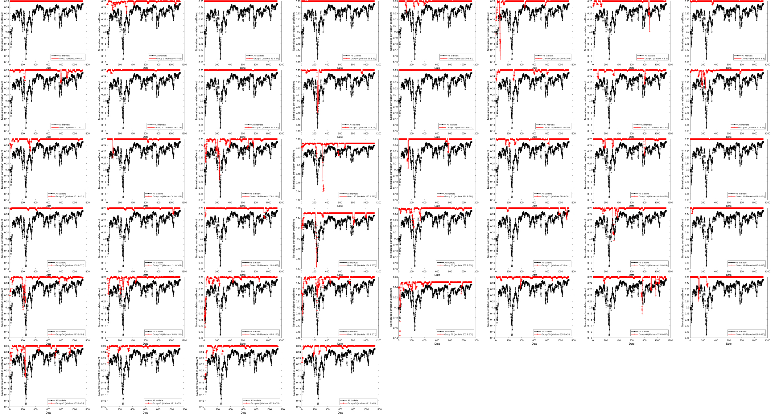
Figure 5 shows the GC for all of the 497 markets (Group 0) and cash markets in Groups 1–58 shown in Table 1, which sheds light on price interactions between all market pairs of a group and thus price comovement information in the group. Particularly, the GC is the sum of all correlation pairs among a number of series under consideration normalized by the number of pairs consistent with the MST. Generally, the higher the GCs, the more similarities. For Group 0 (the dark line in Figure 5), the degree of comovements across all markets is generally higher after March 2008. This is generally consistent with the literature that documents increased price comovements for different commodities (Janzen and Smith 2012; Tang and Xiong 2012).[5] Such a pattern of the increased synchronization is also reported in An et al. 2014; JanzenSt. Louis, Missouri; AgEcon Search and Smith 2012; Ma et al. 2021; Tang and Xiong 2012; Wu et al. 2020; Xiao et al. 2020 for periods close to the financial crisis.[6] Our results extend the evidence to the case of spatially disperse cash markets and the futures market for one single commodity (JanzenSt. Louis, Missouri; AgEcon Search and Smith 2012; Tang and Xiong 2012). However, no persistent increase in the degree of comovements is observed across all markets. This is consistent with the argument of Yang, Li, and Miao (2021a) that the effect of the financialization of commodities might be more limited than previously assumed.[7] For Groups 1–58 (the red line in Figure 5), the price synchronization is rather stable except for only short sub-periods when it slightly drops. Similar empirical evidence is seen from Wu et al. (2020), who find that the dependency for each of three commodity categories, i.e. agriculture products, metal, and energy, generally stabilizes for a sub-period of their analysis. The identification of groups of cash markets with relatively stable synchronizations is meaningful in spatial economic analysis as this indicates that certain policy analysis, e.g. market microstructure and forecasting, related to prices of selected individual cash markets within a specific sectoral group could be better or more precisely conducted. Meanwhile, this could benefit portfolio construction and risk diversification (Peng et al. 2021). The futures, however, is not found to show stable price synchronization with any cash market. And there are no obvious differences in the results between cash markets in the delivery area and those outside the delivery area. This finding suggests a limited informational role of the US corn futures, which could be attributed to the fact that the sample period of this study is around the blatant and widespread failure of US grain futures during 2005–2010 (Garcia, Irwin, and Smith 2015) due to, partly, poor design of delivery terms including delivery warehousing whose importance is discussed in Yang, Li, and Wang (2021b).


GC (Global Correlation). The dark line represents the GC for all of the 497 markets and the red line represents the GC for a specific group reported in Table 1. Dates are from July 19, 2006 to February 17, 2011. The GC is based on the rolling window of 20 days.
Figure 6 shows the SI, which analyzes the rolling importance of different markets in the network. In Figure 6, the horizontal axis shows the dates from July 19, 2006 to February 17, 2011 and the vertical axis shows the markets indexed from 1 to 497, with the cash markets being indexed from 1 to 496 and the futures market indexed as 497. The SI is the number of connections for a price series (associated with a market on the vertical axis of Figure 6) inside the MST weighted by the distance of the connections. Given a rolling window, the SI helps characterize how each series moves within the network over time and whether it turns to be more or less synchronized. One can observe that over time, the SI generally increases, consistent with GC analysis. Similar empirical evidence is found in Matesanz et al. (2014) when they examine price comovements of multiple commodities over the period of December 1992 to July 2010 using monthly data.[8] The results here suggest that spatially disperse corn cash markets generally become more integrated in terms of prices for the period under consideration. There are markets, i.e. the markets showing relatively high levels of synchronization intensities in Figure 6, whose prices appear to be more connected to other prices in the network. These markets could be price leaders in their respective groups (Xu and Zhang 2021b), which might be tested by lead-lag (Xu 2017b, 2018c) and contemporaneous (Xu 2019b; Xu and Zhang 2021c) causality.
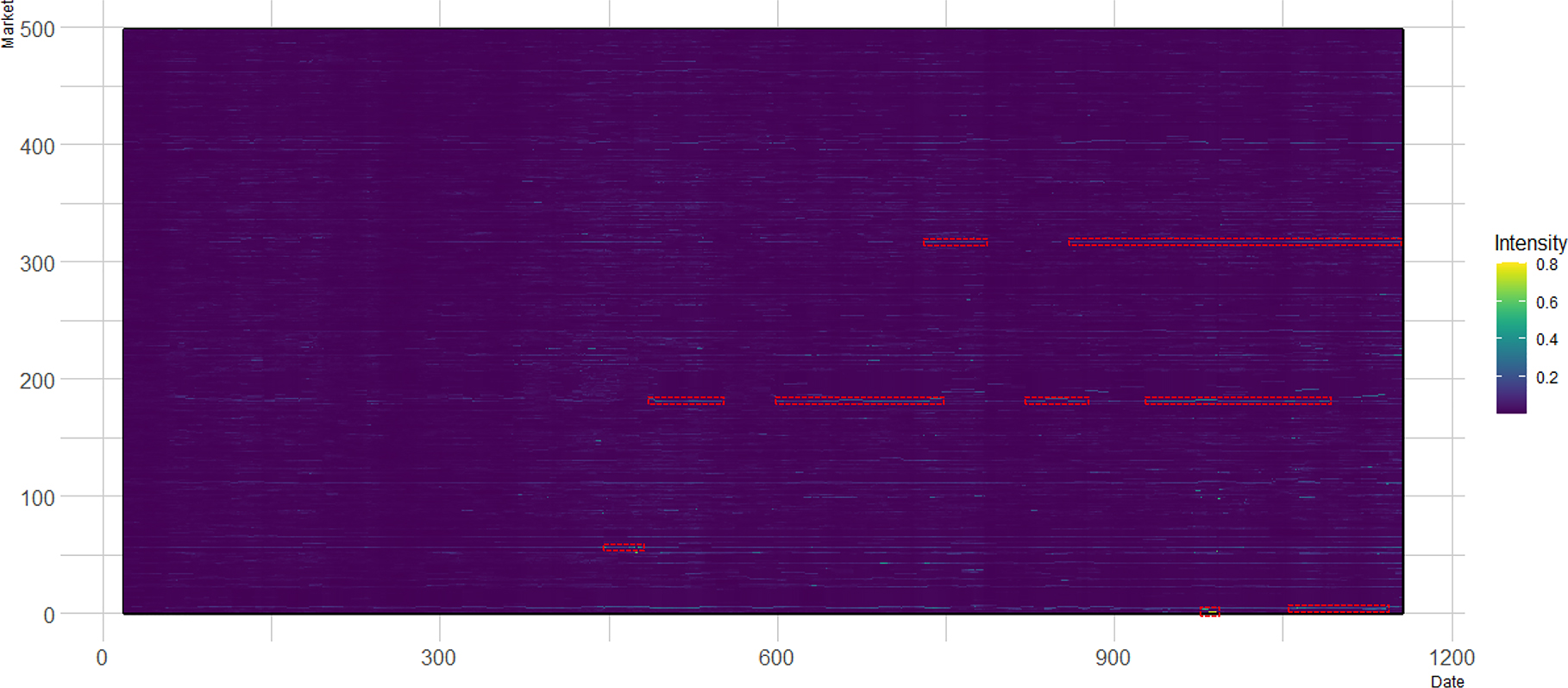
SI (Synchronization Intensity). Dates are from July 19, 2006 to February 17, 2011. Markets are indexed from 1 to 497, with the cash markets being indexed from 1 to 496 and the futures market indexed as 497. The SI is based on the rolling window of 20 days. The red dashed boxes mark several examples for when the SI increases for a market. Referring to the vertical color bar on the rightmost part of this figure, the part of the SI that the red dashed boxes mark is the part with similar colors to the topper part of the vertical color bar.
6 Robustness
6.1 Subsample Analysis
In this subsection, we conduct analysis based on price series of the futures and 355 cash markets in Iowa, Illinois, Nebraska, and Minnesota, which contribute to about 52% of the national harvest acres (USDA-NASS 2010). Locations of the 355 cash markets are shown in Figure 7. In Figures 8 and 9, we show the MST and HT based on the futures and 355 cash markets, which suggest that the results obtained based on the futures and all of the 496 cash markets are generally robust in this subsample with cash markets from the four states. More specifically, we show in Figure 10 the GC analysis based on groups 1–24 and 26–45 shown in Table 1, which is based on the futures and 355 cash markets. We could observe that the GC analysis results are also robust as compared to those shown in Figure 5 that are based on the futures and all of the 496 cash markets. Finally, we present in Figure 11 the SI based on the futures and 355 cash markets. Comparing the results in Figure 11 and those in Figure 6, we could see again that the results obtained based on the futures and all of the 496 cash markets are generally robust in this subsample with cash markets from the four states.

Three hundred fifty five cash markets in Iowa, Illinois, Nebraska, and Minnesota. The cash market index is marked with the blue font inside the red solid circle, representing the location of a cash market.

MST (Minimum Spanning Tree) based on the futures and 355 cash markets in Iowa, Illinois, Nebraska, and Minnesota shown in Figure 7. Please note that the mappings between the numbers in the circles in this figure and the market indices are as follows in the format of “x–y”, where “x” refers to the number in a circle and “y” refers to the market index: 1–4, 2–5, 3–6, 4–7, 5–8, 6–9, 7–10, 8–11, 9–12, 10–13, 11–14, 12–15, 13–16, 14–17, 15–18, 16–19, 17–20, 18–21, 19–22, 20–23, 21–24, 22–25, 23–26, 24–27, 25–28, 26–29, 27–30, 28–31, 29–32, 30–33, 31–34, 32–35, 33–36, 34–37, 35–38, 36–39, 37–40, 38–41, 39–42, 40–43, 41–44, 42–45, 43–46, 44–47, 45–48, 46–49, 47–50, 48–51, 49–52, 50–53, 51–54, 52–55, 53–56, 54–57, 55–58, 56–59, 57–60, 58–61, 59–62, 60–63, 61–64, 62–65, 63–66, 64–67, 65–68, 66–69, 67–70, 68–71, 69–72, 70–73, 71–74, 72–75, 73–76, 74–77, 75–78, 76–79, 77–80, 78–81, 79–82, 80–83, 81–84, 82–85, 83–101, 84–102, 85–103, 86–104, 87–108, 88–109, 89–120, 90–121, 91–122, 92–123, 93–124, 94–125, 95–126, 96–127, 97–128, 98–129, 99–138, 100–139, 101–140, 102–141, 103–142, 104–143, 105–144, 106–145, 107–146, 108–147, 109–148, 110–151, 111–152, 112–154, 113–155, 114–156, 115–157, 116–158, 117–160, 118–161, 119–162, 120–163, 121–164, 122–165, 123–166, 124–167, 125–168, 126–169, 127–170, 128–171, 129–172, 130–178, 131–179, 132–180, 133–181, 134–182, 135–183, 136–184, 137–185, 138–186, 139–187, 140–188, 141–189, 142–190, 143–191, 144–192, 145–193, 146–194, 147–195, 148–196, 149–197, 150–198, 151–199, 152–200, 153–201, 154–202, 155–203, 156–204, 157–205, 158–206, 159–207, 160–208, 161–209, 162–210, 163–211, 164–212, 165–213, 166–214, 167–215, 168–216, 169–217, 170–218, 171–220, 172–221, 173–222, 174–224, 175–225, 176–235, 177–236, 178–237, 179–238, 180–239, 181–240, 182–241, 183–242, 184–243, 185–244, 186–246, 187–248, 188–249, 189–250, 190–251, 191–252, 192–253, 193–254, 194–255, 195–256, 196–257, 197–258, 198–259, 199–260, 200–261, 201–262, 202–264, 203–265, 204–266, 205–268, 206–269, 207–270, 208–271, 209–272, 210–273, 211–274, 212–275, 213–277, 214–279, 215–280, 216–281, 217–282, 218–283, 219–284, 220–285, 221–286, 222–287, 223–288, 224–289, 225–290, 226–291, 227–292, 228–293, 229–294, 230–295, 231–296, 232–297, 233–298, 234–299, 235–300, 236–301, 237–302, 238–303, 239–328, 240–329, 241–330, 242–331, 243–332, 244–333, 245–334, 246–335, 247–336, 248–337, 249–339, 250–340, 251–341, 252–342, 253–343, 254–344, 255–364, 256–365, 257–369, 258–370, 259–371, 260–372, 261–373, 262–374, 263–375, 264–376, 265–377, 266–378, 267–379, 268–380, 269–381, 270–382, 271–383, 272–384, 273–385, 274–386, 275–387, 276–388, 277–389, 278–390, 279–391, 280–392, 281–393, 282–394, 283–401, 284–402, 285–403, 286–404, 287–405, 288–406, 289–407, 290–408, 291–409, 292–410, 293–411, 294–412, 295–413, 296–414, 297–415, 298–416, 299–417, 300–419, 301–427, 302–428, 303–429, 304–430, 305–431, 306–434, 307–435, 308–437, 309–438, 310–439, 311–440, 312–441, 313–442, 314–443, 315–444, 316–447, 317–448, 318–449, 319–450, 320–451, 321–452, 322–453, 323–454, 324–455, 325–456, 326–457, 327–458, 328–459, 329–460, 330–462, 331–463, 332–464, 333–465, 334–466, 335–467, 336–471, 337–472, 338–473, 339–474, 340–476, 341–477, 342–479, 343–480, 344–481, 345–482, 346–484, 347–485, 348–486, 349–487, 350–489, 351–490, 352–491, 353–492, 354–493, 355–494, 356–497 (futures).

GC (Global Correlation) based on groups 1–24 and 26–45 shown in Table 1, which are based on the futures and 355 cash markets in Iowa, Illinois, Nebraska, and Minnesota shown in Figure 7. The dark line represents the GC for all of the 356 markets and the red line represents the GC for a specific group. Dates are from July 19, 2006 to February 17, 2011. The GC is based on the rolling window of 20 days.

SI (Synchronization Intensity) based on the futures and 355 cash markets in Iowa, Illinois, Nebraska, and Minnesota shown in Figure 7. Dates are from July 19, 2006 to February 17, 2011. The SI is based on the rolling window of 20 days.
6.2 Subperiod Analysis
In this subsection, we conduct analysis based on the subperiod of January 4, 2010 – February 17, 2011. In Figures 12 and 13, we show the MST and HT based on this subperiod, which suggest that the results are generally robust when compared with those based on the full sample period. More specifically, we show in Figure 14 the GC analysis based on the 58 groups shown in Table 1, which is based on the subperiod. We could observe that the GC analysis results are also robust as compared to those shown in Figure 5 that are based on the full sample period. We also present in Figure 15 the SI based on the subperiod. Comparing the results in Figure 15 and those in Figure 6, we could see again that the results obtained based on the full sample period are generally robust in the subperiod.

MST (Minimum Spanning Tree) based on the subperiod of January 4, 2010 – February 17, 2011.

HT (Hierarchical Tree) based on the subperiod of January 4, 2010 – February 17, 2011.
GC (Global Correlation). The dark line represents the GC for all of the 497 markets and the red line represents the GC for a specific group reported in Table 1. Dates are from January 4, 2010 to February 17, 2011. The GC is based on the rolling window of 20 days.
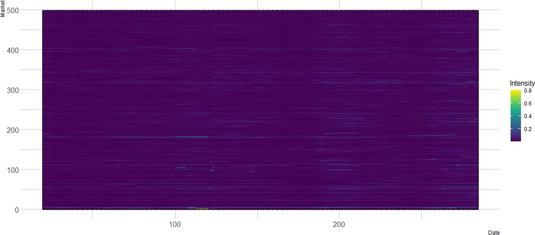
SI (Synchronization Intensity) based on the subperiod of January 4, 2010 – February 17, 2011. The SI is based on the rolling window of 20 days.
We mention before that the futures is not found to show stable price synchronization with any cash market based on the full sample period. And this might be due to the fact that the full sample period of this study is around the blatant and widespread failure of US grain futures during 2005–2010 (Garcia, Irwin, and Smith 2015). More specifically, Garcia, Irwin, and Smith (2015) find that this problem is at its worst during September 2005 – September 2008 and the problem is not really resolved for corn when the time reaches the end of our sample analyzed here, although the problem is not as severe during October 2008 – February 2011. Therefore, the subperiod analysis during January 4, 2010 – February 17, 2011 aims at identifying if the futures potentially shows relatively stable price synchronization with any cash market with the futures failure problem becoming less severe. However, similar to the analysis based on the full sample, we do not find such patterns based on the subperiod either. For example, in Figure 16, we show the GC analysis based on the subperiod for the futures and three cash markets in IL that are found to be relatively close to the futures based on the HT. We could observe that the patterns are generally volatile. If more data become available for periods without the futures failure issue, it would be interesting to further investigate whether the price synchronization between the future and cash markets turns to be more stable.

GC (Global Correlation). The dark line represents the GC for all of the 497 markets and the red line represents the GC for the futures (market 497) and a cash market. Dates are from January 4, 2010 to February 17, 2011. The GC is based on the rolling window of 20 days. The rightmost subfigure shows the locations of the three cash markets.
7 Conclusion
This study analyzes comovements of unique and proprietary daily prices of 496 corn cash markets from 16 states in the United States and the futures market for the period of July 2006 – February 2011 by shedding light on interdependence and synchronization via network analysis and topological and hierarchical characterizations of price dynamics. This empirical framework facilitates endogenous identifications of market groups with similar price synchronization patterns, which could benefit policy analysis regarding commodity prices of individual markets. The framework also enables us to sort out price interactions, allowing for complexities and heterogeneities in price systems.
We find that the degree of comovements is generally higher after March 2008 but no persistent increasing trend is observed. This suggests that there might be supply and demand pattern changes after March 2008 that enhance overall price synchronization. This is generally consistent with the literature that documents increased price comovements for different commodities. Such a pattern of the increased synchronization is also reported in the literature for periods close to the financial crisis. Also similar to the cross-commodity evidence, the elevated corn price synchronization during this period is not permanent. Although not rigorously tested, excessive price comovements might reveal themselves during a similar crisis period. We identify 58 groups of cash markets, each of which has its members generally exhibit similar and stable price dynamics across the sample period. Price synchronization within a certain group also is higher than that across all of the 497 markets. Prices of cash markets in an identified group might be driven by group specific factors in addition to common factors across all markets. The futures, however, is not found to show stable price synchronization with any cash market. Further, we show that certain markets have potential of serving as price leaders because of their increasing connectivities over time with other markets. These price dynamics heterogeneities could be of use to diversify risk and optimize portfolios (Peng et al. 2021; Xu and Zhang 2022a, 2022g).
Finally, we note that the fact that the minimum spanning tree and hierarchical tree methods are rather straightforward is not only their advantage but also potentially their limitation depending on specific research purposes. Particularly, one might not be able to directly comment on causality related questions based on the results (Kristoufek, Janda, and Zilberman 2012). However, network analysis could help identify potential price leaders, which is important part for research on price discovery and information flows as it is essential to select and include such markets in a model for policy analysis involving causality, especially under the data rich environment. For our case, we find that there exist markets, i.e. the markets showing relatively high levels of synchronization intensities, whose prices appear to be more connected to other prices in the network. These markets might be important to be included in studies involving causality analysis and they could possibly be found to be price leaders. A recent study by Yang, Tong, and Yu (2021c) combines two networks, i.e. the directed acyclic graph and popular spillover index of Diebold and Yılmaz (2014), into a unified framework and provides a research direction of utilizing networks for shedding light on causality issues. We also note that the corn yield is an important and interesting topic, although our study focuses on prices and might not directly speak to it. There are previous studies on the relationship between the corn yield and price, such as Houck and Gallagher (1976) on price responses to yields, and Goodwin et al. (2012), Haile, Kalkuhl, and von Braun (2016), and Miao, Khanna, and Huang (2016) on yield responses to prices. It should a worthwhile avenue for future research on yield and price relationships through network analysis, especially under a data rich environment. Finally, inter-cluster analysis also offers an interesting direction to explore for future work.

Prices (cents per bushel) and their first differences of 496 corn cash markets (market index: 1, 2, …, 496) and the futures (497th) market. Dates are from July 19, 2006 to February 17, 2011.


Plots of cash markets in each of the 58 groups shown in Table 1. The cash market index is marked with the blue font inside the red solid circle, representing the location of a cash market.
References
Akpan, U. I., and A. Starkey. 2021. “Review of Classification Algorithms with Changing Inter-Class Distances.” Machine Learning with Applications 4: 100031, https://doi.org/10.1016/j.mlwa.2021.100031.Suche in Google Scholar
Al-Shabandar, R., A. Jaddoa, P. Liatsis, and A. J. Hussain. 2021. “A Deep Gated Recurrent Neural Network for Petroleum Production Forecasting.” Machine Learning with Applications 3: 100013, https://doi.org/10.1016/j.mlwa.2020.100013.Suche in Google Scholar
Alzahrani, M., M. Masih, and O. Al-Titi. 2014. “Linear and Non-Linear Granger Causality Between Oil Spot and Futures Prices: A Wavelet Based Test.” Journal of International Money and Finance 48: 175–201, https://doi.org/10.1016/j.jimonfin.2014.07.001.Suche in Google Scholar
Amato, J. D., and N. R. Swanson. 2001. “The Real-Time Predictive Content of Money for Output.” Journal of Monetary Economics 48: 3–24, https://doi.org/10.1016/S0304-3932(01)00070-8.Suche in Google Scholar
An, H., X. Gao, W. Fang, Y. Ding, and W. Zhong. 2014. “Research on Patterns in the Fluctuation of the Co-Movement Between Crude Oil Futures and Spot Prices: A Complex Network Approach.” Applied Energy 136: 1067–75, https://doi.org/10.1016/j.apenergy.2014.07.081.Suche in Google Scholar
An, S., X. Gao, H. An, S. Liu, Q. Sun, and N. Jia. 2020. “Dynamic Volatility Spillovers Among Bulk Mineral Commodities: A Network Method.” Resources Policy 66: 101613, https://doi.org/10.1016/j.resourpol.2020.101613.Suche in Google Scholar
Anderson, T. W., and D. A. Darling. 1954. “A Test of Goodness of Fit.” Journal of the American Statistical Association 49: 765–9.10.1080/01621459.1954.10501232Suche in Google Scholar
Ashley, R. A., and K. P. Tsang. 2014. “Credible Granger-Causality Inference with Modest Sample Lengths: A Cross-Sample Validation Approach.” Econometrics 2: 72–91, https://doi.org/10.3390/econometrics2010072.Suche in Google Scholar
Awokuse, T. O. 2007. “Market Reforms, Spatial Price Dynamics, and China’s Rice Market Integration: A Causal Analysis with Directed Acyclic Graphs.” Journal of Agricultural and Resource Economics 32: 58–76.Suche in Google Scholar
Balcombe, K., A. Bailey, and J. Brooks. 2007. “Threshold Effects in Price Transmission: The Case of Brazilian Wheat, Maize, and Soya Prices.” American Journal of Agricultural Economics 89: 308–23, https://doi.org/10.1111/j.1467-8276.2007.01013.x.Suche in Google Scholar
Batarseh, F. A., M. Gopinath, A. Monken, and Z. Gu. 2021. “Public Policymaking for International Agricultural Trade Using Association Rules and Ensemble Machine Learning.” Machine Learning with Applications 5: 100046, https://doi.org/10.1016/j.mlwa.2021.100046.Suche in Google Scholar
Bekiros, S. D., and C. G. Diks. 2008. “The Relationship Between Crude Oil Spot and Futures Prices: Cointegration, Linear and Nonlinear Causality.” Energy Economics 30: 2673–85, https://doi.org/10.1016/j.eneco.2008.03.006.Suche in Google Scholar
Bera, A. K., and C. M. Jarque. 1981. “Efficient Tests for Normality, Homoscedasticity and Serial Independence of Regression Residuals: Monte Carlo Evidence.” Economics Letters 7: 313–8, https://doi.org/10.1016/0165-1765(81)90035-5.Suche in Google Scholar
Bessler, D. A., and D. G. Akleman. 1998. “Farm Prices, Retail Prices, and Directed Graphs: Results for Pork and Beef.” American Journal of Agricultural Economics 80: 1144–9, https://doi.org/10.2307/1244220.Suche in Google Scholar
Bessler, D. A., and J. Yang. 2003. “The Structure of Interdependence in International Stock Markets.” Journal of International Money and Finance 22: 261–87, https://doi.org/10.1016/S0261-5606(02)00076-1.Suche in Google Scholar
Bessler, D. A., J. Yang, and M. Wongcharupan. 2003. “Price Dynamics in the International Wheat Market: Modeling with Error Correction and Directed Acyclic Graphs.” Journal of Regional Science 43: 1–33, https://doi.org/10.1111/1467-9787.00287.Suche in Google Scholar
Chopra, A., and D. A. Bessler. 2005. “Price Discovery in the Black Pepper Market in Kerala, India.” Indian Economic Review 40: 1–21.Suche in Google Scholar
Cooper, M., R. C. GutierrezJr, and B. Marcum. 2005. “On the Predictability of Stock Returns in Real Time.” The Journal of Business 78: 469–500, https://doi.org/10.1086/427635.Suche in Google Scholar
Corea, F., G. Bertinetti, and E. M. Cervellati. 2021. “Hacking the Venture Industry: An Early-Stage Startups Investment Framework for Data-Driven Investors.” Machine Learning with Applications 5: 100062, https://doi.org/10.1016/j.mlwa.2021.100062.Suche in Google Scholar
Cramér, H. 1928. “On the Composition of Elementary Errors: First Paper: Mathematical Deductions.” Scandinavian Actuarial Journal 1928: 13–74, https://doi.org/10.1080/03461238.1928.10416862.Suche in Google Scholar
De Boor, C. 1978. A Practical Guide to Splines, Vol. 27. New York: Springer-Verlag.10.1007/978-1-4612-6333-3Suche in Google Scholar
Dickey, D. A., and W. A. Fuller. 1981. “Likelihood Ratio Statistics for Autoregressive Time Series with a Unit Root.” Econometrica 49: 1057–72, https://doi.org/10.2307/1912517.Suche in Google Scholar
Diebold, F. X., and K. Yılmaz. 2014. “On the Network Topology of Variance Decompositions: Measuring the Connectedness of Financial Firms.” Journal of Econometrics 182: 119–34, https://doi.org/10.1016/j.jeconom.2014.04.012.Suche in Google Scholar
Esposti, R., and G. Listorti. 2013. “Agricultural Price Transmission Across Space and Commodities During Price Bubbles.” Agricultural Economics 44: 125–39, https://doi.org/10.1111/j.1574-0862.2012.00636.x.Suche in Google Scholar
Ferraro, D., K. Rogoff, and B. Rossi. 2015. “Can Oil Prices Forecast Exchange Rates? An Empirical Analysis of the Relationship Between Commodity Prices and Exchange Rates.” Journal of International Money and Finance 54: 116–41, https://doi.org/10.1016/j.jimonfin.2015.03.001.Suche in Google Scholar
Flori, A., F. Pammolli, and A. Spelta. 2021. “Commodity Prices Co-Movements and Financial Stability: A Multidimensional Visibility Nexus with Climate Conditions.” Journal of Financial Stability 54: 100876, https://doi.org/10.1016/j.jfs.2021.100876.Suche in Google Scholar
Garbade, K. D., and W. L. Silber. 1983. “Price Movements and Price Discovery in Futures and Cash Markets.” The Review of Economics and Statistics 65: 289–297, https://doi.org/10.2307/1924495.Suche in Google Scholar
Garcia, P., S. H. Irwin, and A. Smith. 2015. “Futures Market Failure?” American Journal of Agricultural Economics 97: 40–64, https://doi.org/10.1093/ajae/aau067.Suche in Google Scholar
Gonzalo, J., and C. Granger. 1995. “Estimation of Common Long-Memory Components in Cointegrated Systems.” Journal of Business & Economic Statistics 13: 27–35, https://doi.org/10.2307/1392518.Suche in Google Scholar
Goodwin, B. K., M. C. Marra, N. E. Piggott, and S. Müeller. 2012. Is Yield Endogenous to Price? An Empirical Evaluation of Inter- and Intra-Seasonal Corn Yield Response. Technical Report. Seattle, Washington: AgEcon Search.Suche in Google Scholar
Goodwin, B. K., and N. E. Piggott. 2001. “Spatial Market Integration in the Presence of Threshold Effects.” American Journal of Agricultural Economics 83: 302–17, https://doi.org/10.1111/0002-9092.00157.Suche in Google Scholar
Gower, J. C. 1966. “Some Distance Properties of Latent Root and Vector Methods Used in Multivariate Analysis.” Biometrika 53: 325–38, https://doi.org/10.1093/biomet/53.3-4.325.Suche in Google Scholar
Haigh, M. S., and D. A. Bessler. 2004. “Causality and Price Discovery: An Application of Directed Acyclic Graphs.” The Journal of Business 77: 1099–121, https://doi.org/10.1086/422632.Suche in Google Scholar
Haile, M. G., M. Kalkuhl, and J. von Braun. 2016. “Worldwide Acreage and Yield Response to International Price Change and Volatility: A Dynamic Panel Data Analysis for Wheat, Rice, Corn, and Soybeans.” American Journal of Agricultural Economics 98: 172–90, https://doi.org/10.1093/ajae/aav013.Suche in Google Scholar
Hasbrouck, J. 1995. “One Security, Many Markets: Determining the Contributions to Price Discovery.” The Journal of Finance 50: 1175–99, https://doi.org/10.1111/j.1540-6261.1995.tb04054.x.Suche in Google Scholar
Helbling, T., V. Mercer-Blackman, and K. Cheng. 2008. “Riding a Wave.” Finance and Development 45: 10–5.Suche in Google Scholar
Hidalgo, C. A., and R. Hausmann. 2009. “The Building Blocks of Economic Complexity.” Proceedings of the National Academy of Sciences 106: 10570–5, https://doi.org/10.1073/pnas.0900943106.Suche in Google Scholar
Houck, J. P., and P. W. Gallagher. 1976. “The Price Responsiveness of US Corn Yields.” American Journal of Agricultural Economics 58: 731–4, https://doi.org/10.2307/1238817.Suche in Google Scholar
Hu, M., D. Zhang, Q. Ji, and L. Wei. 2020. “Macro Factors and the Realized Volatility of Commodities: A Dynamic Network Analysis.” Resources Policy 68: 101813, https://doi.org/10.1016/j.resourpol.2020.101813.Suche in Google Scholar
Janzen, J. P., and A. D. Smith. 2012. Commodity Price Comovement: The Case of Cotton. St. Louis, Missouri: AgEcon Search.Suche in Google Scholar
Jarque, C. M., and A. K. Bera. 1980. “Efficient Tests for Normality, Homoscedasticity and Serial Independence of Regression Residuals.” Economics Letters 6: 255–9, https://doi.org/10.1016/0165-1765(80)90024-5.Suche in Google Scholar
Javed, A., B. S. Lee, and D. M. Rizzo. 2020. “A Benchmark Study on Time Series Clustering.” Machine Learning with Applications 1: 100001, https://doi.org/10.1016/j.mlwa.2020.100001.Suche in Google Scholar
Johnson, S. C. 1967. “Hierarchical Clustering Schemes.” Psychometrika 32: 241–54, https://doi.org/10.1007/BF02289588.Suche in Google Scholar
Kang, S. H., A. K. Tiwari, C. T. Albulescu, and S. M. Yoon. 2019. “Exploring the Time-Frequency Connectedness and Network Among Crude Oil and Agriculture Commodities v1.” Energy Economics 84: 104543, https://doi.org/10.1016/j.eneco.2019.104543.Suche in Google Scholar
Kolmogorov, A. 1933. “Sulla determinazione empirica di una lgge di distribuzione.” Giornale dell’Istituto Italiano degli Attuari 4: 83–91.Suche in Google Scholar
Kristoufek, L., K. Janda, and D. Zilberman. 2012. “Correlations Between Biofuels and Related Commodities Before and During the Food Crisis: A Taxonomy Perspective.” Energy Economics 34: 1380–91, https://doi.org/10.1016/j.eneco.2012.06.016.Suche in Google Scholar
Kristoufek, L., K. Janda, and D. Zilberman. 2013. “Regime-Dependent Topological Properties of Biofuels Networks.” The European Physical Journal B 86: 1–12, https://doi.org/10.1140/epjb/e2012-30871-9.Suche in Google Scholar
Kruskal, J. B. 1956. “On the Shortest Spanning Subtree of a Graph and the Traveling Salesman Problem.” Proceedings of the American Mathematical Society 7: 48–50, https://doi.org/10.2307/2033241.Suche in Google Scholar
Kuiper, W. E., C. Lutz, and A. Van Tilburg. 1999. “Testing for the Law of One Price and Identifying Price-Leading Markets: An Application to Corn Markets in Benin.” Journal of Regional Science 39: 713–38, https://doi.org/10.1111/0022-4146.00157.Suche in Google Scholar
Kwiatkowski, D., P. C. Phillips, P. Schmidt, and Y. Shin. 1992. “Testing the Null Hypothesis of Stationarity Against the Alternative of a Unit Root.” Journal of Econometrics 54: 159–78, https://doi.org/10.1016/0304-4076(92)90104-Y.Suche in Google Scholar
Lee, C. C., and J. H. Zeng. 2011. “Revisiting the Relationship Between Spot and Futures Oil Prices: Evidence from Quantile Cointegrating Regression.” Energy Economics 33: 924–35, https://doi.org/10.1016/j.eneco.2011.02.012.Suche in Google Scholar
Ma, Y. R., Q. Ji, F. Wu, and J. Pan. 2021. “Financialization, Idiosyncratic Information and Commodity Co-Movements.” Energy Economics 94: 105083, https://doi.org/10.1016/j.eneco.2020.105083.Suche in Google Scholar
Matesanz, D., B. Torgler, G. Dabat, and G. J. Ortega. 2014. “Co-Movements in Commodity Prices: A Note Based on Network Analysis.” Agricultural Economics 45: 13–21, https://doi.org/10.1111/agec.12126.Suche in Google Scholar
Miao, R., M. Khanna, and H. Huang. 2016. “Responsiveness of Crop Yield and Acreage to Prices and Climate.” American Journal of Agricultural Economics 98: 191–211, https://doi.org/10.1093/ajae/aav025.Suche in Google Scholar
Minoiu, C., and J. A. Reyes. 2013. “A Network Analysis of Global Banking: 1978–2010.” Journal of Financial Stability 9: 168–84, https://doi.org/10.1016/j.jfs.2013.03.001.Suche in Google Scholar
Miśkiewicz, J., and M. Ausloos. 2010. “Has the World Economy Reached its Globalization Limit?” Physica A: Statistical Mechanics and its Applications 389: 797–806, https://doi.org/10.1016/j.physa.2009.10.029.Suche in Google Scholar
Oellermann, C. M., B. B. Wade, and P. L. Farris. 1989. “Price Discovery for Feeder Cattle.” The Journal of Futures Markets (1986–1998) 9: 113, https://doi.org/10.1002/fut.3990090204.Suche in Google Scholar
Peng, Y., P. H. M. Albuquerque, H. Kimura, and C. A. P. B. Saavedra. 2021. “Feature Selection and Deep Neural Networks for Stock Price Direction Forecasting Using Technical Analysis Indicators.” Machine Learning with Applications 5: 100060, https://doi.org/10.1016/j.mlwa.2021.100060.Suche in Google Scholar
Phillips, P. C., and P. Perron. 1988. “Testing for a Unit Root in Time Series Regression.” Biometrika 75: 335–46, https://doi.org/10.1093/biomet/75.2.335.Suche in Google Scholar
Piesse, J., and C. Thirtle. 2009. “Three Bubbles and a Panic: An Explanatory Review of Recent Food Commodity Price Events.” Food Policy 34: 119–29, https://doi.org/10.1016/j.foodpol.2009.01.001.Suche in Google Scholar
Reyes, J., S. Schiavo, and G. Fagiolo. 2010. “Using Complex Networks Analysis to Assess the Evolution of International Economic Integration: The Cases of East Asia and Latin America.” The Journal of International Trade & Economic Development 19: 215–39, https://doi.org/10.1080/09638190802521278.Suche in Google Scholar
Rossi, B. 2013. “Advances in Forecasting Under Instability.” In Handbook of Economic Forecasting, Vol. 2, 1203–324. Elsevier.10.1016/B978-0-444-62731-5.00021-XSuche in Google Scholar
Schroeder, T. C., and B. K. Goodwin. 1991. “Price Discovery and Cointegration for Live Hogs.” The Journal of Futures Markets (1986–1998) 11: 685, https://doi.org/10.1002/fut.3990110604.Suche in Google Scholar
Schwarz, T. V., and A. C. Szakmary. 1994. “Price Discovery in Petroleum Markets: Arbitrage, Cointegration, and the Time Interval of Analysis.” The Journal of Futures Markets (1986–1998) 14: 147, https://doi.org/10.1002/fut.3990140204.Suche in Google Scholar
Sephton, P. S. 2003. “Spatial Market Arbitrage and Threshold Cointegration.” American Journal of Agricultural Economics 85: 1041–6, https://doi.org/10.1111/1467-8276.00506.Suche in Google Scholar
Shapiro, S. S., and M. B. Wilk. 1965. “An Analysis of Variance Test for Normality (Complete Samples).” Biometrika 52: 591–611, https://doi.org/10.2307/2333709.Suche in Google Scholar
Shimizu, S., P. O. Hoyer, A. Hyvärinen, A. Kerminen, and M. Jordan. 2006. “A Linear Non-Gaussian Acyclic Model for Causal Discovery.” Journal of Machine Learning Research 7: 2003–2030.Suche in Google Scholar
Shimizu, S., T. Inazumi, Y. Sogawa, A. Hyvärinen, Y. Kawahara, T. Washio, P. O. Hoyer, and K. Bollen. 2011. “Directlingam: A Direct Method for Learning a Linear Non-Gaussian Structural Equation Model.” The Journal of Machine Learning Research 12: 1225–48.Suche in Google Scholar
Shu, J., and J. E. Zhang. 2012. “Causality in the Vix Futures Market.” Journal of Futures Markets 32: 24–46, https://doi.org/10.1002/fut.20506.Suche in Google Scholar
Silvapulle, P., and I. A. Moosa. 1999. “The Relationship Between Spot and Futures Prices: Evidence from the Crude Oil Market.” Journal of Futures Markets: Futures, Options, and Other Derivative Products 19: 175–93, https://doi.org/10.1002/(SICI)1096-9934(199904)19:2¡175::AID-FUT3¿3.0.CO;2-H.10.1002/(SICI)1096-9934(199904)19:2<175::AID-FUT3>3.3.CO;2-8Suche in Google Scholar
Smirnov, N. V. 1939. “Estimate of Deviation Between Empirical Distribution Functions in Two Independent Samples.” Bulletin Moscow University 2: 3–16.Suche in Google Scholar
Swanson, N. R., and C. W. Granger. 1997. “Impulse Response Functions Based on a Causal Approach to Residual Orthogonalization in Vector Autoregressions.” Journal of the American Statistical Association 92: 357–67, https://doi.org/10.1080/01621459.1997.10473634.Suche in Google Scholar
Tang, K., and W. Xiong. 2012. “Index Investment and the Financialization of Commodities.” Financial Analysts Journal 68: 54–74, https://doi.org/10.2469/faj.v68.n6.5.Suche in Google Scholar
Tao, L., and F. M. Song. 2010. “Do Small Traders Contribute to Price Discovery? Evidence from the Hong Kong Hang Seng Index Markets.” Journal of Futures Markets: Futures, Options, and Other Derivative Products 30: 156–74, https://doi.org/10.1002/fut.20410.Suche in Google Scholar
USDA-NASS. 2010. Field Crops Usual Planting and Harvesting Dates, 1–51. National Agriculture Statistics Services.Suche in Google Scholar
Verma, P., and R. Goyal. 2021. “Influence Propagation Based Community Detection in Complex Networks.” Machine Learning with Applications 3: 100019, https://doi.org/10.1016/j.mlwa.2020.100019.Suche in Google Scholar
Von Mises, R. 1928. Statistik und wahrheit, Vol. 20. Julius Springer.Suche in Google Scholar
Wang, Z., J. Yang, and Q. Li. 2007. “Interest Rate Linkages in the Eurocurrency Market: Contemporaneous and Out-of-Sample Granger Causality Tests.” Journal of International Money and Finance 26: 86–103, https://doi.org/10.1016/j.jimonfin.2006.10.005s.Suche in Google Scholar
Wasserman, S., and K. Faust. 1994. Social Network Analysis: Methods and Applications, 8. Cambridge: Cambridge University Press.10.1017/CBO9780511815478Suche in Google Scholar
Wu, F., W. L. Zhao, Q. Ji, and D. Zhang. 2020. “Dependency, Centrality and Dynamic Networks for International Commodity Futures Prices.” International Review of Economics & Finance 67: 118–32, https://doi.org/10.1016/j.iref.2020.01.004.Suche in Google Scholar
Xiao, B., H. Yu, L. Fang, and S. Ding. 2020. “Estimating the Connectedness of Commodity Futures Using a Network Approach.” Journal of Futures Markets 40: 598–616, https://doi.org/10.1002/fut.22086.Suche in Google Scholar
Xu, X. 2015. “Cointegration Among Regional Corn Cash Prices.” Economics Bulletin 35: 2581–94.Suche in Google Scholar
Xu, X. 2017a. “Contemporaneous Causal Orderings of US Corn Cash Prices Through Directed Acyclic Graphs.” Empirical Economics 52: 731–58, https://doi.org/10.1007/s00181-016-1094-4.Suche in Google Scholar
Xu, X. 2017b. “The Rolling Causal Structure Between the Chinese Stock Index and Futures.” Financial Markets and Portfolio Management 31: 491–509, https://doi.org/10.1007/s11408-017-0299-7.Suche in Google Scholar
Xu, X. 2017c. “Short-Run Price Forecast Performance of Individual and Composite Models for 496 Corn Cash Markets.” Journal of Applied Statistics 44: 2593–620, https://doi.org/10.1080/02664763.2016.1259399.Suche in Google Scholar
Xu, X. 2018a. “Causal Structure Among US Corn Futures and Regional Cash Prices in the Time and Frequency Domain.” Journal of Applied Statistics 45: 2455–80, https://doi.org/10.1080/02664763.2017.1423044.Suche in Google Scholar
Xu, X. 2018b. “Cointegration and Price Discovery in US Corn Cash and Futures Markets.” Empirical Economics 55: 1889–923, https://doi.org/10.1007/s00181-017-1322-6.Suche in Google Scholar
Xu, X. 2018c. “Intraday Price Information Flows Between the Csi300 and Futures Market: An Application of Wavelet Analysis.” Empirical Economics 54: 1267–95, https://doi.org/10.1007/s00181-017-1245-2.Suche in Google Scholar
Xu, X. 2018d. “Linear and Nonlinear Causality Between Corn Cash and Futures Prices.” Journal of Agricultural & Food Industrial Organization 16: 20160006, https://doi.org/10.1515/jafio-2016-0006.Suche in Google Scholar
Xu, X. 2018e. “Using Local Information to Improve Short-Run Corn Price Forecasts.” Journal of Agricultural & Food Industrial Organization 16: 20170018, https://doi.org/10.1515/jafio-2017-0018.Suche in Google Scholar
Xu, X. 2019a. “Contemporaneous and Granger Causality Among US Corn Cash and Futures Prices.” European Review of Agricultural Economics 46: 663–95, https://doi.org/10.1093/erae/jby036.Suche in Google Scholar
Xu, X. 2019b. “Contemporaneous Causal Orderings of Csi300 and Futures Prices Through Directed Acyclic Graphs.” Economics Bulletin 39: 2052–77.Suche in Google Scholar
Xu, X. 2019c. “Price Dynamics in Corn Cash and Futures Markets: Cointegration, Causality, and Forecasting Through a Rolling Window Approach.” Financial Markets and Portfolio Management 33: 155–81, https://doi.org/10.1007/s11408-019-00330-7.Suche in Google Scholar
Xu, X. 2020. “Corn Cash Price Forecasting.” American Journal of Agricultural Economics 102: 1297–320, https://doi.org/10.1002/ajae.12041.Suche in Google Scholar
Xu, X., and Y. Zhang. 2021a. “Corn Cash Price Forecasting with Neural Networks.” Computers and Electronics in Agriculture 184: 106120, https://doi.org/10.1016/j.compag.2021.106120.Suche in Google Scholar
Xu, X., and Y. Zhang. 2021b. “House Price Forecasting with Neural Networks.” Intelligent Systems with Applications 12: 200052, https://doi.org/10.1016/j.iswa.2021.200052.Suche in Google Scholar
Xu, X., and Y. Zhang. 2021c. “Individual Time Series and Composite Forecasting of the Chinese Stock Index.” Machine Learning with Applications 5: 100035, https://doi.org/10.1016/j.mlwa.2021.100035.Suche in Google Scholar
Xu, X., and Y. Zhang. 2021d. “Network Analysis of Corn Cash Price Comovements.” Machine Learning with Applications 6: 100140, https://doi.org/10.1016/j.mlwa.2021.100140.Suche in Google Scholar
Xu, X., and Y. Zhang. 2021e. “Rent Index Forecasting Through Neural Networks.” Journal of Economic Studies, https://doi.org/10.1108/JES-06-2021-0316.Suche in Google Scholar
Xu, X., and Y. Zhang. 2021f. “Second-Hand House Price Index Forecasting with Neural Networks.” Journal of Property Research, https://doi.org/10.1080/09599916.2021.1996446.Suche in Google Scholar
Xu, X., and Y. Zhang. 2022a. “Coking Coal Futures Price Index Forecasting with the Neural Network.” Mineral Economics, https://doi.org/10.1007/s13563-022-00311-9.Suche in Google Scholar
Xu, X., and Y. Zhang. 2022b. “Commodity Price Forecasting via Neural Networks for Coffee, Corn, Cotton, Oats, Soybeans, Soybean Oil, Sugar, and Wheat.” Intelligent Systems in Accounting, Finance and Management, https://doi.org/10.1002/isaf.1519.Suche in Google Scholar
Xu, X., and Y. Zhang. 2022c. “Contemporaneous Causality Among One Hundred Chinese Cities.” Empirical Economics, https://doi.org/10.1007/s00181-021-02190-5.Suche in Google Scholar
Xu, X., and Y. Zhang. 2022d. “Contemporaneous Causality Among Residential Housing Prices of Ten Major Chinese Cities.” International Journal of Housing Markets and Analysis, https://doi.org/10.1108/IJHMA-03-2022-0039.Suche in Google Scholar
Xu, X., and Y. Zhang. 2022e. “Forecasting the Total Market Value of a Shares Traded in the Shenzhen Stock Exchange via the Neural Network.” Economics Bulletin.Suche in Google Scholar
Xu, X., and Y. Zhang. 2022f. “Network Analysis of Housing Price Comovements of a Hundred Chinese Cities.” National Institute Economic Review, https://doi.org/10.1017/nie.2021.34.Suche in Google Scholar
Xu, X., and Y. Zhang. 2022g. “Residential Housing Price Index Forecasting via Neural Networks.” Neural Computing and Applications, https://doi.org/10.1007/s00521-022-07309-y.Suche in Google Scholar
Xu, X., and Y. Zhang. 2022h. “Soybean and Soybean Oil Price Forecasting Through the Nonlinear Autoregressive Neural Network (narnn) and Narnn with Exogenous Inputs (narnn–x).” Intelligent Systems with Applications 13: 200061, https://doi.org/10.1016/j.iswa.2022.200061.Suche in Google Scholar
Xu, X., and Y. Zhang. 2022i. “Thermal Coal Price Forecasting via the Neural Network.” Intelligent Systems with Applications 14: 200084, https://doi.org/10.1016/j.iswa.2022.200084.Suche in Google Scholar
Yang, J., and D. A. Bessler. 2004. “The International Price Transmission in Stock Index Futures Markets.” Economic Inquiry 42: 370–86, https://doi.org/10.1093/ei/cbh067.Suche in Google Scholar
Yang, J., D. A. Bessler, and D. J. Leatham. 2001. “Asset Storability and Price Discovery in Commodity Futures Markets: A New Look.” Journal of Futures Markets 21: 279–300, https://doi.org/10.1002/1096-9934(200103)21:3¡279::AID-FUT5¿3.0.CO;2-L.10.1002/1096-9934(200103)21:3<279::AID-FUT5>3.3.CO;2-CSuche in Google Scholar
Yang, J., and D. J. Leatham. 1999. “Price Discovery in Wheat Futures Markets.” Journal of Agricultural and Applied Economics 31: 359–70, https://doi.org/10.22004/ag.econ.15375.Suche in Google Scholar
Yang, J., Z. Li, and H. Miao. 2021a. “Volatility Spillovers in Commodity Futures Markets: A Network Approach.” Journal of Futures Markets 41: 1959–87, https://doi.org/10.1002/fut.22270.Suche in Google Scholar
Yang, J., Z. Li, and T. Wang. 2021b. “Price Discovery in Chinese Agricultural Futures Markets: A Comprehensive Look.” Journal of Futures Markets 41: 536–55, https://doi.org/10.1002/fut.22179.Suche in Google Scholar
Yang, J., M. Tong, and Z. Yu. 2021c. “Housing Market Spillovers Through the Lens of Transaction Volume: A New Spillover Index Approach.” Journal of Empirical Finance 64: 351–78, https://doi.org/10.1016/j.jempfin.2021.10.003.Suche in Google Scholar
Zhang, D., and G. Z. Fan. 2019. “Regional Spillover and Rising Connectedness in China’s Urban Housing Prices.” Regional Studies 53: 861–73, https://doi.org/10.1080/00343404.2018.1490011.Suche in Google Scholar
Zhang, D., Q. Ji, W. L. Zhao, and N. J. Horsewood. 2021. “Regional Housing Price Dependency in the UK: A Dynamic Network Approach.” Urban Studies 58: 1014–31, https://doi.org/10.1177/0042098020943489.Suche in Google Scholar
Zhong, W., R. Kong, and G. Chen. 2019. “Gold Prices Fluctuation of Co-Movement Forecast Between China and Russia.” Resources Policy 62: 218–30, https://doi.org/10.1016/j.resourpol.2019.03.012.Suche in Google Scholar
© 2022 Walter de Gruyter GmbH, Berlin/Boston
Artikel in diesem Heft
- Frontmatter
- Research Articles
- Private Supply Management and Market Power in the U.S. Dairy Industry
- Implementing Antitrust Regulations in Dynamic Industries: The Case of the U.S. Cottonseed Industry
- Price Hedonics of Beers: Effects of Alcohol Content, Quality Rating, and Production Country
- Olive Oil World Price Forecasting: A Bayesian VAR Approach
- Network Analysis of Price Comovements Among Corn Futures and Cash Prices
- Evaluating Impacts of Subsidy Removal in the Tunisian Bakery Sector
- Mark Ups and Pass-Through in Small and Medium Retailers for Rice, Tomato Sauce and Oil