Discrete Morse theory segmentation on high-resolution 3D lithic artifacts
-
Jan Philipp Bullenkamp

 ,
Theresa Kaiser
,
Theresa Kaiser

Abstract
Motivated by the question of understanding the roots of tool making by anatomically modern humans and coexisting Neanderthals in the Paleolithic, a number of shape classification methods have been tested on photographs and drawings of stone tools. Since drawings contain interpretation and photographs fool both human and computational methods by color and shadows on the surface, we propose an approach using 3D datasets as best means for analyzing shape, and rely on first open access repositories on lithic tools. The goal is to not only analyze shape on an artifact level, but allow a more detailed analysis of stone tools on a scar and ridge level. A Morse-Smale complex (MS complex) extracted from the triangular mesh of a 3D model is a reduced skeleton consisting of linked lines on the mesh. Discrete Morse theory makes it possible to obtain such a MS complex from a scalar function. Thus, we begin with Multi-Scale Integral Invariant filtering on the meshes of lithic artifacts, which provides curvature measures for ridges, which are convex, and scars, which are concave. The resulting values on the vertices can be used as our discrete Morse function and the skeleton we get is build up from lines that will coincide with the ridges and, implicitly, contains the scars as enclosed regions of those lines on the mesh. As this requires a few parameters, we provide a graphical user interface (GUI) to allow altering the predefined parameters to quickly find a good result. In addition, a stone tool may have areas that do not belong to the scar/ridge class. These can be masked and we use conforming MS complexes to ensure that the skeleton keeps these areas whole. Finally, results are shown on real and open access datasets. The source code and manually annotated ground truth for the evaluation are provided as Open Access with a Creative Commons license.
1 Introduction
In the Old Stone Age, Paleolithic, the name-giving stone tools are one of the central classes of objects that give us insight into the habits of early humans. All human species, from Homo habilis and Homo erectus to Homo neanderthalensis and anatomically modern humans (AMHs), have at one time or another used stone tools to cut, scrape, or pierce other objects. Because of their resilience and durability, stone tools are often preserved in the archaeological record, giving us the opportunity to study their diversity in detail. Stone tools are one of the few types of artifacts found in the Paleolithic record. Because of this limitation, this field has focused almost exclusively on the study of lithic artifacts.
For the production of stone tools, also known as knapping, several hammerstones or antlers, often also anvils and a nodule of raw material are needed. While hitting or applying pressure to the nodule, pieces flake off from its surface, leaving negative imprints, so-called scars, which are surrounded by ridges. With each step, the scar pattern becomes more complex, resulting in an artifact as shown in Figure 1. In the analysis of stone artifacts, each scar represents an impact and provides evidence of either an intentional action or a natural process, such as weathering [1], [2]. This clear relationship between an object and a production step is easily observable and almost unique for seeing ancient action so clearly. Segmenting and analyzing the scars of stone artifacts is therefore a central question for understanding Paleolithic people and is giving us insights into the concept behind the applied technical pattern.
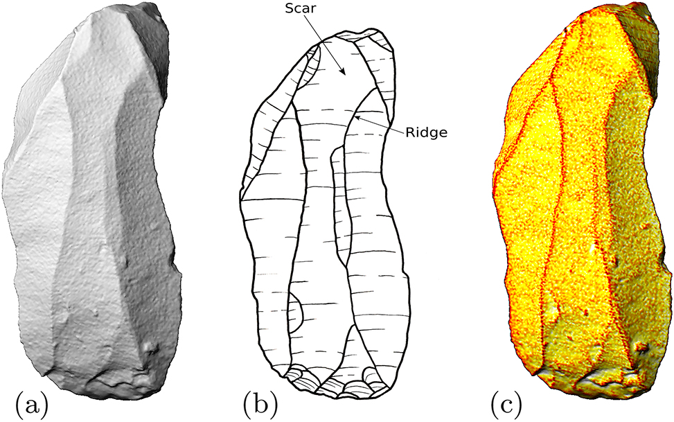
Images of the artifact 31, (a) orthographic projection of the scanned object; (b) drawing of artifact; (c) MSII-curvature mapped as function value.
Today’s archaeological approach is to visually recognize the shape and scar patterns of artifacts and manually draw, for example, the contour line and ridges. All drawings are by their nature unique projections of a 3D object onto a 2D image, and inherently interpreted based on previous points. Some artifacts are upscaled or downscaled in this process, further distorting the original dimensions of the artifacts. All spatial properties and ratios are unreliable due to the intrinsic limitation of interpreted drawings and should not be used whenever other data is either available or can be collected. Therefore, there is an urgent need to transfer the knowledge from a 2D perspective to a more generalized 3D approach using 3D annotations, where each scar is annotated directly on the surface of the model. 3D annotations are rare in archaeology, and only a handful of approaches, e.g., [3], have successfully implemented it.
Due to the high demand for analytical approaches, the publications of Artifact GeoMorph Toolbox3-D (AGMT3-D) by Herzlinger and Grosman [4] and Artifact3-D software by Grosman et al. [5] were created to add new possibilities for analyzing 3D models of stone artifacts. Even the use of neural networks to simulate knapping has been published by Orellana et al. [6]. One of the underrepresented and understudied aspects is still the question of scar segmentation. To date, there is to our knowledge only one paper that focuses on the quantitative analysis of drawn artifacts and their scars by Gellis et al. [7] and one article by Richardson et al. [8], which explores this challenge for 3D models.
In this paper, we present our user-guided method for segmenting lithic artifacts to address the need for manual segmentation. Our approach will be based on Morse theory [9] which is used to calculate the topology of a manifold by studying a scalar function on it. It possesses a discrete counterpart, which was introduced by Forman [10] and thereby allows to use it on discrete datasets such as triangular meshes of 3D models. Numerous algorithms [11], [12] now allow to calculate a so-called Morse complex, giving us a skeletonized version of the mesh we are looking at. This leads to many applications [13] including segmentations of, e.g., trees from point clouds of terrestrial laser scanning [14]. Looking for the required scalar function, the so-called Morse function, curvature values seem a good choice, as the worked scars usually have a smooth slightly concave surface, while the ridges characteristically are a sharp convex edge. Therefore we use the curvature values computing Multi-Scale Integral Invariant (MSII) filtering [15]. An example of a MSII filter result is shown in Figure 1(c) and used as input function for our proposed method based on Morse theory.
Some artifacts are only partially knapped and do have unworked areas, also called cortex, though. These areas usually have a very rough surface, so the curvature values will vary between very convex and very concave parts posing a challenge for the segmentation using curvature values as input for our Morse theory algorithm. This leads to an additional option allowing users to add pre-labeling of rough areas.
As a case study, we selected 62 3D models from the Grotta di Fumane (GdF), an open source data repository of lithic artifacts [16], and manually segmented them for our ground truth dataset. These were produced by AMHs belonging to the Proto-Aurignacian (41,000 − 37,000 cal BP) [17], [18].
2 Discrete Morse theory
Morse theory [9] goes back to the calculus of variations in the large, a work by Marston Morse in the late twenties of the last century. In it, he developed a powerful differential topology technique for classifying critical points on a manifold by its unstable submanifolds. This technique requires only a so-called Morse function defined on this manifold, which is differentiable and has no degenerate critical points. For today’s applications on discretized surfaces representing a 2D manifold, the continuous theory has a discrete counterpart [10], and there is no longer any need to detour to the continuous case with sufficiently differentiable functions on smooth surfaces.
2.1 Discrete Morse function
A mesh describing the surface of a 3D object can also be considered as a simplicial complex consisting of the measured vertices (0-simplices), the edges (1-simplices) between these vertices and the triangles formed by the edges (2-simplices). Such a mesh must also be a 2D manifold in the sense that it looks locally like a plane with no self-intersections or edges that are part of more than two triangles. To obtain a discrete vector field, we first need a real function defined on the set of vertices. This can be, e.g., the curvature at each vertex. For technical reasons, we need to make sure that no vertex has exactly the same value as another vertex, see [12] for details. This function is our discrete Morse function, and any function that has different values at each vertex will do the job. The function is extended from the vertices to the edges and triangles, by assigning each simplex the lexicographically ordered values of its bounding vertices in decreasing order.
2.2 Discrete vector field
A lower star of a 0-simplex is all simplices with lower values that have a direct connection to this vertex, so all simplices whose assigned function value starts with the function value of the vertex. The lower stars are disjoint, but the union of all the lower stars forms the original mesh. The lexicographic order makes sure that within each lower star, every simplex is ranked below all of its faces. We now process the lower stars, and this can be done in parallel, without regard to the order of the vertices. A so-called pairing is performed in this process, and the pair with the steepest descent is written into the discrete vector field. Since all vertices have different values, there is at most a single edge to a vertex with the smallest value. If there is no such vertex, we are already in a sink and this vertex is a critical simplex, also called a minimum. There could be other edges in a lower star, which are not yet paired with a vertex, and also triangles with an unpaired edge, so the pairing continues. From a triangle with a single free, i.e. unpaired, edge, we can descend via the edge with the lowest values. The triangle and edge are paired and written to the discrete vector field. One triangle after the other in the lower star gets to a priority queue with just a single free edge. If an edge remains that cannot be paired, this is a critical simplex, a so-called saddle. In the case of a triangle that has no free edge left, we are dealing with a critical simplex that is a maximum. This way we iterate through all the lower stars and end up with a set of critical simplices (minima, saddles and maxima) and a discrete vector field in form of pairings (α (p), β (p+1)) between vertex and edge or edge and triangle, where the superscripts denote the dimension of the simplices α and β. It follows quite naturally that the dimension of the critical simplices also means the assignment to one of the three possibilities: minimum (0D), saddle (1D) or maximum (2D). Figure 2 shows a part of a mesh with the vector field pairings indicated by arrows. In this case we chose the labeling of the vertices as Morse function, which automatically provides us with unique function values. A critical triangle {18, 17, 16} is marked in blue, two critical edges {13, 10} and {9, 7} are marked in green and two critical vertices {0} and {1} are marked in red.

A discrete vector field on a mesh with the vertex indices giving the Morse function, e.g., the edge {9, 7} has the lexicographical function value {9, 7}. The critical triangle is marked in blue, critical edges in green, critical vertices in red and simplices that are part of the separatrices are marked in pink.
2.3 Separatrices
The pairings in the discrete vector field can be seen as a combinatorial gradient on the simplicial complex. There are either pairings from a vertex to an edge or from an edge to a triangle, both indicating a decreasing function value in that direction. The unpaired critical simplices, so the maxima, saddles and minima, describe points of the function with vanishing gradient, e.g., extreme points.
A so-called V-path is defined as an alternating sequence of p- and (p + 1)-dimensional simplices, starting at a (p + 1)-dimensional simplex s (p+1) and descending to a p-dimensional simplex d (p)
where
Special cases are V-paths between critical simplices, in our case from critical triangles to critical edges or from critical edges to critical vertices: those are called separatrices. Naturally critical simplices offer themselves as starting and destination simplices for V-paths, as they resemble points with gradient zero and are not contained in any pairing in the discrete vector field and thereby mark end points of a V-path.
To find a separatrix, we start at a critical (p + 1)-simplex and look at its faces (or borders), which are p-simplices. We then check each of them, if it is a critical simplex, which would already return a separatrix, or otherwise we check if it is part of a (α (p), β (p+1)) pairing in the discrete vector field, in which case we repeat the search starting with the (p + 1)-simplex it is pointing to.
Note that there can be several separatrices originating in the same critical simplex, and there can be several separatrices terminating in one critical simplex, so when looking for separatrices, a breadth-first search is required and multiple traversals of each simplex need to be allowed, see [12] for details.
So for example in Figure 2 starting at the critical edge {9, 7} in green, we look at the two vertices {9} and {7}, which are the faces of this edge, and follow the directions implied by the vector field pairings of these vertices: {9, 2} and {7, 6} in this case. The first separatrix continues from the other face of the edge {9, 2}, the vertex {2}, along the edge {2, 1} to the critical vertex {1} and we have a separatrix given by the alternating sequence {9, 7}, {9}, {9, 2}, {2}, {2, 1}, {1} between the two critical simplices {9, 7} and {1}. The other separatrix takes one more discrete vector field pairing until it terminates in the critical vertex {0}: {9, 7}, {7}, {7, 6}, {6}, {6, 5}, {5}, {5, 0}, {0}.
It is guaranteed that every path terminates either by not finding a critical simplex and resulting in a dead end or by finding a critical simplex and creating a separatrix, because the Morse function value strictly decreases in each step and our meshes naturally have a minimal function value.
Remark: Note that only separatrices from critical edges to critical vertices can merge, as there might be several vertices, whose paired edges point towards the same vertex, as for, e.g., the edges {13, 8} and {11, 8} in Figure 2 both pointing to the vertex {8}. If the edge {11, 8} would be another separatrix here, this would consequently merge these two separatrices. These saddle-minimum separatrices are not able to split up though, as each edge in the separatrix has two vertices as faces, and one vertex is the direction the separatrix is coming from, while the other can only be paired with at most one edge in the discrete vector field, permitting a splitting separatrix here.
Separatrices from critical triangles to critical edges cannot merge, as we deal with manifold like surfaces, so we do not allow any edge to have more than two adjacent triangles, which would be necessary to join two different separatrices into one. But a maximim-saddle separatrix can split, as a triangle has three faces (edges): one edge needs to be the direction the separatrix is coming from and if both other edges are paired with triangles, the separatrix can continue in two directions. In Figure 2 take the path that originates in the critical triangle {18, 17, 16} and starts from the edge {18, 17}, which is paired with the triangle {18, 17, 15}: this path now splits and continues with the edge {18, 15} to the triangle {18, 15, 12} but also with the edge {17, 15} to the triangle {17, 15, 6}. In this case the latter will be a dead end, as it stops in the triangle {17, 5, 0} and the first path terminates in the critical edge {9, 7} forming a separatrix between two critical simplices.
2.4 Discrete Morse-Smale complexes
In algebraic topology the definition of a chain complex allows to compute the homology of a given mesh. Such a chain complex consists of a sequence of abelian groups
A Morse-Smale complex (MS complex) is defined as such a chain complex, by taking the critical simplices from the discrete Morse function as well as the separatrices connecting them. The abelian groups for the chain complex are defined as the vector spaces spanned by the critical simplices of the corresponding dimension. Since we are working on a mesh, we only have dimensions 0, 1 and 2 and thus our chain complex also reduces to these three groups with A i = 0 otherwise. So the critical vertices span the chain group A 0, critical edges A 1 and critical triangles A 2.
The boundary maps d 0: A 1 → A 0 and d 1: A 2 → A 1 can be defined from the two types of separatrices. There are two separatrices originating in a critical edge going to critical vertices, so d 0 maps a critical edge in A 1 to those critical vertices. Similarly d 1 maps a critical triangle to the critical edges it is connected to by separatrices. The exact definitions require the introduction of orientation to make sure that the boundary homomorphisms also satisfy d 0◦d 1 = 0, so for more details we refer to Ref. [10].
For topological computations and analysis, this abstract algebraic complex suffices and depicts the correct topology of the mesh independent from the chosen Morse function. Considering the mesh geometry as well, the abstract boundary information of how critical simplices connect to each other is not enough, therefore a geometric MS complex also contains the separatrices between them to give the actual paths of these connections. We will only work with the geometric MS complexes from now on, so we always include the geometric information given by the separatrices when speaking of MS complexes.
Looking at a surface embedded in 3D, the geometric MS complex then looks like a skeleton on the simplicial complex and separates it into different regions. These regions are called Morse cells and represent areas where the discrete Morse function behaves monotonically. Figure 3 schematically depicts such a MS complex for the example from Figure 2 with the maximum in blue, saddles in green, minima in red and their separatrices in pink. We then have different Morse cells (enclosures) that are depicted in different colors.
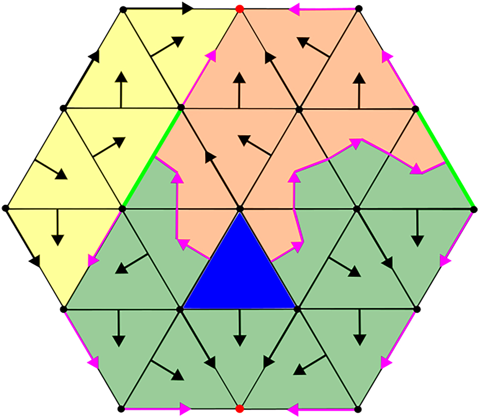
Morse complex and Morse cells: critical triangle (maxima) in blue, critical edges (saddles) in green, critical vertices (minima) in red and separatrices in pink; Morse cells are filled in different colors.
2.5 Simplification
The initial MS complexes usually contain noise, so there are local minima, saddles and maxima that make the complex very fine grained. Edelsbrunner et al. [19] introduced the concept of persistence which allows to remove noise and simplify a complex in a topologically consistent way. Persistence generally describes the longevity of topological features which can be imagined as the lifetime of a feature, like a connected component that is later merged with another, when gradually constructing a complex by a rising function value threshold.
The persistence of a critical simplex is defined as the smallest function value difference to another critical simplex connected with a separatrix. To compare the lexicographically ordered tuples of different lengths for the critical simplices as function values we take the maximal function value in each tuple and take their difference.
If we have two critical simplices connected with a separatrix, that have a low persistence, we can cancel the critical simplices by reversing the pairings along the separatrix, but only if there is a single separatrix between the two critical simplices. Otherwise we would retract a loop and thereby destroy the topological consistency of the MS complex. The reversal along a separatrix can be done by splitting up all pairings and taking the starting and destination simplices into the chain, reversing the flow direction. So an original separatrix from a critical simplex s (p+1) to critical simplex d (p) one dimension below with indicated vector field pairings
would be split up and reversed to the following pairings
As we can see by the missing critical simplices at the beginning and end of this V-path, it is now part of other separatrices, that reconnect the other separatrices that previously originated or ended in the cancelled critical simplices. Figure 4 shows such a reversal schematically.

Cancellation of a critical vertex and a critical edge in the center. The reconnected separatrices including the reversed separatrix are shown in orange and two separatrices were removed.
Note how reversing the separatrix and cancelling the two critical simplices, reconnects or cuts the other separatrices that previously originated or ended in those simplices. For the saddle-minimum pair here, the separatrices between the two critical triangles and the cancelled saddle are removed and the separatrices from other saddles to the cancelled minimum are extended via the reversed separatrix to the other minimum that was connected to cancelled saddle. The removed separatrices lead to the merging of Morse cells, that were previously split by those separatrices, so the simplified skeleton also leads to larger Morse cells.
2.6 Conforming Morse-Smale complexes
Conforming Morse-Smale complexes allow to introduce user control to Morse theory based algorithms. They were introduced by Gyulassy et al. [20]. In this setting, we have a user-defined labeling, a function I that assigns a value to each simplex in some finite set S. In Ref. [20], S is defined to be a set of whole numbers, but taking any finite set is equivalent and allows us to do a useful construction. A discrete vector field is called conforming to I if it only pairs up simplices with the same label. A MS complex is conforming to I if it stems from a conforming vector field.
To construct a conforming vector field, we start as before, with an initial real-valued function with unique values on the vertices of the mesh. Additionally, we have the labeling I. Now we can construct a discrete vector field by treating each lower star separately, and traversing its simplices in the same order as in the usual case described in the beginning, but only pairing up simplices with the same I-label. A conforming MS complex can then be extracted from the resulting vector field with the same algorithm as before. This algorithm will yield the same result as the original one, if all simplices have the same label. In most other cases we will have more unpaired, i.e. critical, simplices, making the MS complex bigger, but separating the different labels with separatrices.
If we want to reduce the complex with the same methods as in Section 2.5, we cannot be sure if the resulting complex is conforming again: Through the flipping of a separatrix, simplices with different I-labels might be paired. This can be prevented by only choosing pairs of critical simplices for cancellation that are connected by a single separatrix which only contains simplices with the same label.
2.7 Choice of labeling
Different labelings can be useful for different application. In our case, we want to use conforming MS complexes to influence the segmentation of the mesh into Morse cells such that it respects predefined regions on the vertices.
We start with an initial labeling I on the vertices. We can then extend it to higher dimensional simplices as follows: Given a p-simplex α with vertices {v 0, v 1, …v p }, we define I(α) as the set of the labels of the vertices {I(v 0), I(v 1), …, I(v p )}. This means that labels are not counted twice, they appear at most once in the I(α).
Then a simplex in which all vertices have the same label can be paired with any of its faces, whereas a 2-simplex with two different labels can only be paired with its unique edge with the same two labels. A 2-simplex with three different labels cannot be paired with any of its edges (they cannot have more than two labels) and must be marked as critical, marking a place where three different regions meet. An edge with two different labels cannot be paired with any of its end points, because they only have a single label, which prevents the creation of a path across label borders.
This will ensure that regions of different labels will be surrounded by separatrices on the borders. Within a Morse cell, all vertices will have the same label. This property stays intact even after conforming reduction.
This is illustrated in Figure 5, which shows part of a mesh in which the vertices have labels in {{yellow}, {orange}, {grey}}. This means that an edge has a label within {{yellow}, {orange}, {grey}, {yellow, orange}, {yellow, grey}, {orange, grey}}.

Labels that are extended from vertices to all simplices.
A 2-simplex can have any of those labels or also the label {yellow, orange, grey}.
Pairings only occur for simplices with the same label, so within a uniformly colored region. The slim strips of “two-colored” simplices will contain the separatrices separating the “one-colored” regions, starting and ending (or joining) at critical two-colored edges or 2-simplices or at three-colored 2-simplices, which are all critical.
3 Segmentation method
Our goal is to segment scars of lithic artifacts, which are separated by ridges. Using curvature values as discrete Morse function on the vertices gives us higher values at the convex ridges and lower values in the flat or slightly concave scar areas. Ignoring noise for the moment, the discrete vector field then generates critical triangles, i.e. maxima, at the ridges and critical vertices, i.e. minima, in the scar regions. Separatrices follow extremal lines, so they will often lie on ridges or in valleys. Therefore, the MS complex skeleton naturally already contains the ridges we are looking for. Moreover, the induced Morse cells yield a segmentation that respects the ridges, which are part of the MS complex skeleton.
Also taking into account the noise, the discrete vector field produces a lot of critical simplices including local maxima in flat areas or local minima on ridges. The initial MS complex is a very fine-grained skeleton and the Morse cells therefore are a strong oversegmentation of the scars.
Thus, a few steps are needed to make it work on real data. The segmentation method we introduce is based on the separatrices that can be used to find ridges and the Morse cells that give us a segmentation. We explain each step, starting with the ridge detection from the separatrices in Section 3.1, followed by an oversegmentation performed using the Morse cells in Section 3.2 and finally merging cells based on the found ridges to get a final segmentation result of the scars in Section 3.3.
The method is designed to allow additional user input in form of a pre-labeling that has to be respected. Hence, it expects a conforming Morse-Smale complex as input and returns a vertex-based segmentation of the mesh. In case of no initial labeling this is equal to a normal Morse-Smale complex.
3.1 Ridge extraction
Ridge extraction plays a crucial role for getting a good segmentation result. Since the separatrices between critical simplices represent extremal lines in terms of curvature, they can be used to get thin and connected ridges. Especially separatrices from maxima to saddles are more likely to be a desired ridge than a separatrix from a saddle to a minimum. Those are usually following a valley into a local minimum (sink), which is not what we are looking for. Therefore, we need to introduce a measure defining the importance of a separatrix and how likely it will be a ridge.
Weinkauf and Günther [21] have defined a separatrix persistence p sep by taking the distance of the points on the separatrix sep to the closest other extremum of the saddle point. For points on a maximum-saddle separatrix, the distance to the closest minimum of the saddle point is taken and for a minimum-saddle separatrix, the distance to the closest maximum of the saddle is taken. This would penalize separatrices, that might be on a ridge, but do not have a large distance to the next minimum. Hence we take the average Morse function value along the separatrix as importance measure
where the function values f(x) for simplices x in a separatrix are defined as the maximal value in the lexicographic function value tuple. So for a maximum-saddle separatrix which only consists of triangles and edges, the highest function value of each simplex is taken, for saddle-minimum separatrices we can just take the function values of the vertices, which contains the highest function values of the edges already. Figure 6 shows both separatrix types in our example and marks the vertices that give the function values for the separatrix persistence in red. This tackles another problem as well, since separatrices are defined abstractly as triangle-edge sequences or edge-vertex sequences. In order to get vertex based representations one can just take the vertices of the maximal function value for each simplex as well. Connecting these vertices also gives the separatrices in a vertex based representation: Figure 6 shows the abstract separatrices in pink and the new vertex based separatrices are marked as red edges. For edge-vertex separatrices these are equivalent, but for triangle-edge separatrices we now have a representation that also separates the Morse cells properly without cutting through triangles.

Vertex based representation of saddle-minimum and maximum-saddle separatrices in red (old separatrices in pink), as well as the Morse cells in a vertex based complex.
Filtering the separatrices of the initial MS complex only results in rather small line segments that often are not quite connected to each other. We use the simplification concept introduced in Section 2.5 to reduce the skeleton. In the process, some separatrices are cut off and deleted, while others are reversed and prolonged. We repeatedly cancel critical simplices up to the highest persistence, which results in a minimal MS complex of the mesh. If the mesh is topologically equivalent to a sphere, which means that we have a watertight mesh with no holes in a topological sense, the minimal MS complex consists of a critical vertex and a critical triangle and no separatrices left at all. In the process of getting there, the separatrices of the initial skeleton get longer and longer until they are cut off in a cancellation step, so in practice we simplify the MS complex to a minimal complex and store the separatrices of various lengths in the process. Thresholding those separatrices now returns line segments of various lengths and especially the longer ones can bridge smaller gaps where the curvature value drops below a threshold.
Compared to a classical thresholding on the curvature values only, this approach can not only bridge smaller gaps with lower values, but also returns thin lines immediately and does not require a non-maximum suppression.
Similar to common Canny edge detectors, we use a double threshold
3.2 Oversegmentation
Due to the initially very fine-grained MS complex, the initial Morse cells are very small and not well suited as an oversegmentation. The benefit of using Morse cells lies in the nature of their boundaries: since they originate from the MS complex, the boundaries of a Morse cell are the separatrices and therefore coincide with the detected ridges. Therefore using Morse cells as an oversegmentation makes sure, that the cells do not grow over the detected ridges, but naturally keep them as cell separators.
Using a small persistence value to simplify the MS complex and to reduce noise, gives the option to adapt the level of oversegmentation, such that it is not as fine as the initial Morse cells, but still not merging different scars.
When working with user input, the choice of labeling for the conforming MS complex ensures that within each Morse cell, all vertices have the same label. During the simplification, only critical simplices with equal labels are allowed to be cancelled in order to prevent violating the initial user labeling in the Morse cells. In other words, the initial oversegmentation given by the conforming MS complex does not cross the scars that were predefined by the user.
Since the segmentation works vertex based, the Morse cells are also only filled with the containing vertices. This is done by first adding all vertices that are clearly within a Morse cell and adding the boundaries, so the vertices from simplices on a separatrix, in a second step. There can be Morse cells that do not contain any vertex inside, i.e. if all vertices are considered on the boundary. In those cases we just ignore this Morse cell and add the boundary vertices to the Morse cells on the other side of the boundary.
3.3 Merging
Using the oversegmentation and the detected ridges, scars are found by iteratively merging the oversegmentation together into scars based on the detected ridges. Therefore, we create a weighted adjacency graph of our oversegmentation from the slightly simplified Morse cells. The adjacency of a cell is given by the neighbor cells and the weight between two cells is defined as the percentage of ridge points along their boundary: So for two adjacent cells M i and M j the boundary ∂ ij between them consists of the vertices in M i that are adjacent to at least one vertex in M j together with the vertices in M j that are adjacent to at least one vertex in M i . If an initial labeling is given as user input for conforming Morse cells, we ensure that cells containing different labels I(M i ) ≠ I(M j ) are never merged by setting their weight to +∞. Cells belonging to a scar that was already marked by the user are all merged to form that scar, so the weight of two cells with the same label that has been selected is set to −∞. Thus, the weight between M i and M j is defined as
where R are the ridges points and R ∩ ∂ ij thereby defines the ridge points on the boundary between M i and M j .
Now cells are iteratively merged as long as there are adjacencies with a weight below a threshold. So cells are merged until all cells have a significant amount of ridge detected as boundary towards all neighbor cells and this gives the final scar segmentation. The process is shown schematically in Figure 7: First the blue and gray cells as well as red and green cells are merged as they have no detected ridge points between them. Then green and orange are merged as they have only a little bit of ridge between them. Blue and green are not merged as they only have a little gap in the ridge between them and the percentage of ridge points along their boundary is large enough.

Cells are merged based on the detected ridges.
4 Application
This sections provides comments that are helpful for the implementation and usage of our proposed method. This includes a graphical user interface (GUI) assisting users to swiftly find correct segmentation parameters, namely the high and low ridge detection thresholds, the persistence for the noise removal and reduction of the MS complex and its cells as well as the merging threshold. Additional comments for the guided segmentation with conforming MS complexes are given.
4.1 Implementation
Our implementation uses Python and is available as Open Access using a GNU GPLv3 license https://github.com/JanPhilipp-Bullenkamp/MorseMesh [22]. For the construction of the discrete vector field and the MS complex we follow the pseudocode from the ProcessLowerStars and ExtractMorseComplex algorithms in Ref. [12]. To ensure the required unique function values for these algorithms we add very small values to the duplicate function values, making sure every function value occurs only once. We adapt the ExtractMorseComplex to not only find the connections between critical simplices but also store the paths connecting them, namely the separatrices, as we not only need an abstract MS complex, but a geometrical one that can be used for our segmentation method. Some comments on the persistence reduction algorithm are made in Ref. [11]. Note that we are once again not only interested in the abstract simplification, but also in the cut off and reversed separatrices, so we additionally store those and their separatrix persistences to be able to extract the ridges.
In Algorithm 1 the steps to get a segmentation from a simplicial complex with given four required parameters: persistence, the two ridge thresholds and the merging threshold are shown. GetMorseComplex and the reduce method for a MS complex are adapted from the algorithms mentioned previously. The GetRidges, GetMorseCells and Merge functions correspond to the Sections 3.1–3.3. Getting the Morse complex and reducing it up to a certain persistence are the most time consuming steps here, so it makes sense to store the reduced Morse complex while testing different ridge detection and merge thresholds.
Algorithm 1.
Segmentation(C, p, t h , t l , m).
| Input: C simplicial complex |
| p persistence |
| t h high ridge threshold |
| t l low ridge threshold |
| m merge threshold |
| Output: S Segmentation of vertices |
| 1: MSC = GetMorseComplex(C) |
| 2: ridges = GetRidges(MSC.Separatrices, t h , t l ) |
| 3: redMSC = MSC.reduce(p) |
| 4: cells = GetMorseCells(redMSC) |
| 5: S = Merge(cells, ridges, m) |
4.2 Setting parameters with the GUI
A segmentation depends on four parameters, but their significance differs: while the persistence parameter and merging threshold are not that important, especially the ridge detection parameters determine the outcome of a segmentation. Finding the right parameters especially for ridge detection can be eased using a graphical user interface. Developing such a tool nowadays can be supported using AI: since the creation of basic elements of a GUI are frequently asked in the internet, we were able to use ChatGPT to help creating our tool.
The ridge detection just needs to threshold the separatrices, making it quite fast and can be done in real time. So to find good ridges, it is sufficient to load a mesh into the GUI and compute the Morse complex once which then allows to use sliders to adjust the ridges in real time getting visual feedback on the loaded mesh directly as in Figure 8.
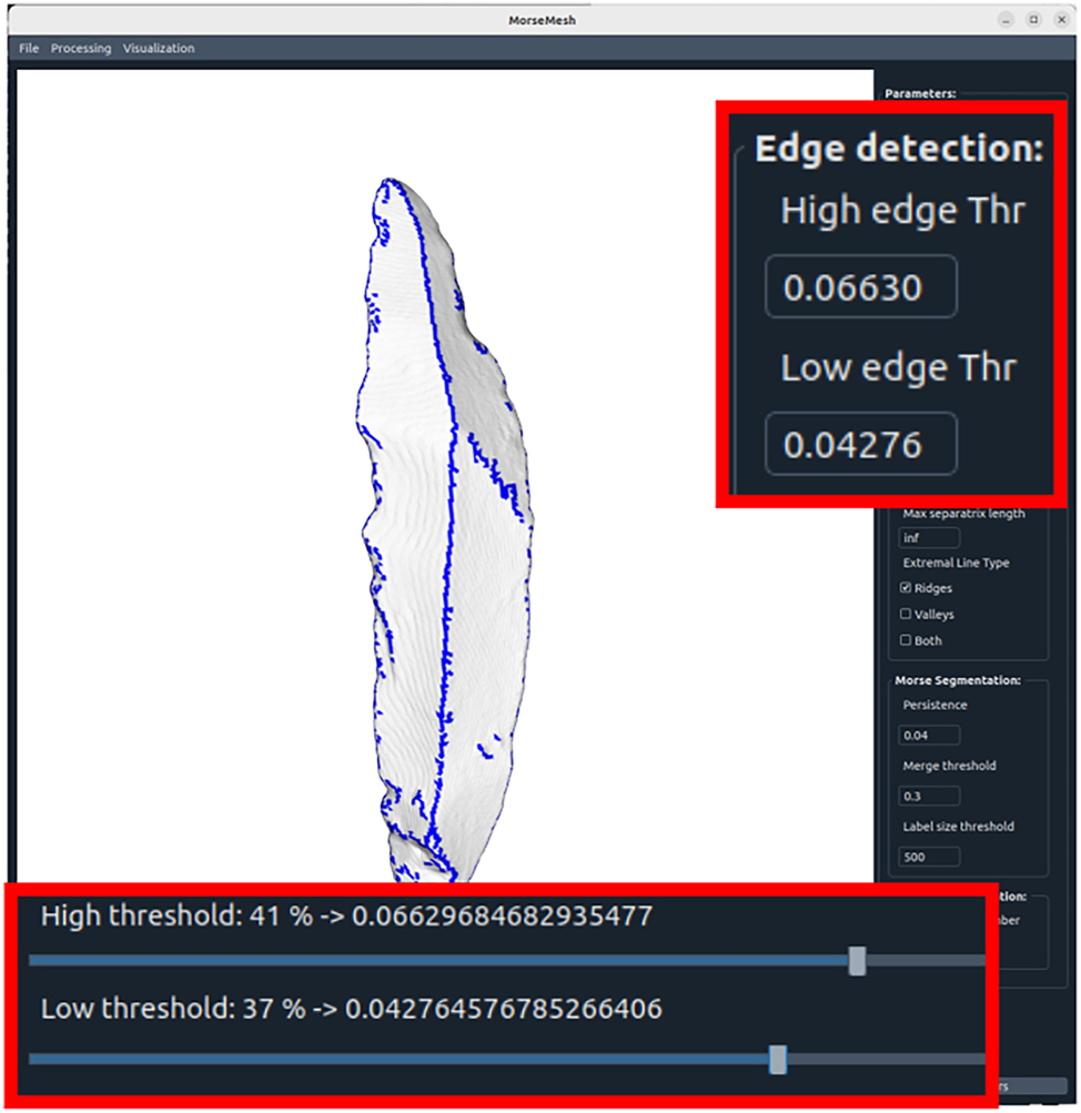
Ridge detection parameters can be found using sliders or input boxes, while seeing the impact on the mesh.
Once good ridge detection thresholds are found, the lithic artifact can be segmented using the persistence parameter and the merging threshold, which can often be fixed for several artifacts. The result is then visualized in the GUI, shown in Figure 9, and can either be saved or the segmentation is run again with different parameters.

Segmentation parameters can be set using input boxes.
4.3 Conforming user input
When working with the user-guided segmentation, a manual segmentation needs to be done, e.g., in Meshlab with the paintbrush tool. It requires a mesh with different colors where each color represents one label and by default will segment the largest label into scars with our method, while keeping the smaller labels as given by the user. An example of this is shown in Figure 10.

The artifacts GdF 700 and 4501 with user input. In each, the blue area will be segmented by the algorithm while the red/purple ones will be kept as marked by the user.
5 Dataset
For the evaluation of our approach, we choose an open-data publication of 3D models [16] of Upper Paleolithic stone artifacts from the GdF in northeastern Italy. This dataset (version 1.0.0) is used to evaluate the accuracy and reliability of our method. The already mentioned AGMT3-D [23] used a subset of this dataset as well to perform a 3D analysis.
GdF is a site commonly associated with the transition from Neanderthals to AMHs [24]. Like many other sites, GdF was occupied by multiple human groups with different ways of producing stone artifacts. GdF is famously associated with the Uluzzian – a transitional industry. According to today’s view, the Uluzzian is one of the earliest technological units of the AMHs in Europe [18], but this view is not uncontroversial. The stone tools taken into account in this study are from the Proto-Aurignacian [16]. The Proto-Aurignacian is considered to belong to the Aurignacian Complex, which is the first Upper Paleolithic techno-complex in Europe and is clearly associated with AHMs. Large bladelets are a marker for the Proto-Aurignacian [25]. The dataset of the open access publication contains only complete blades and bladelets from the Proto-Aurignacian [16].
Hence, for our interest, we will focus mainly on artifacts from the A1-A2 unit, which is dated between 42,000 and 39,250 cal BP, but will also include 5 artifacts from the D3 unit (D3b, D3d and D3d base), which is dated between 40,000 and 37,750 cal BP [17], [18].
Due to the time consuming nature of the manual annotation, we selected 62 out of the 732 artifacts. To manually annotate these 3D models, we used Meshlab’s paintbrush tool [26]. The annotations were used as our ground truths and we make them available for open access [27]. To reflect the diversity of the dataset, we selected a similar number of the two main blanks – blades and bladelets, included artifacts with rather simple and rather complex scar patterns and artifacts with varying amounts of cortex, which is the original outer surface of the unworked raw material. The chosen meshes roughly contain between 40,000 and 400,000 vertices.
6 Results
We introduce a segmentation method containing four parameters: two thresholds (high and low) for the ridge detection, a persistence for the oversegmentation and a merging threshold to get the final result. Figure 11 shows the steps of a segmentation on the artifact 31 from our introduction in Figure 1. In practice the GUI tool shown in Section 4.2 will help finding the best parameters especially for the ridge detection as this step can be visualized and adapted in real-time.
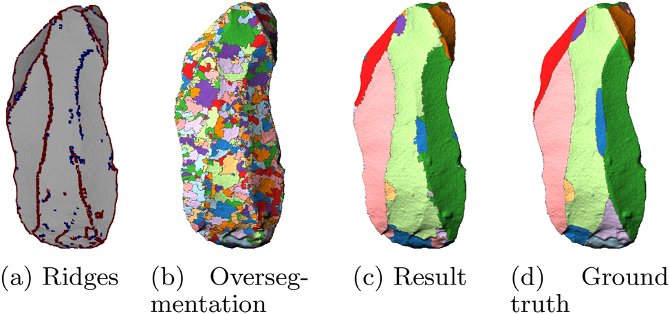
Artifact 31 (a) Double thresholded ridges: strong ridges (red), weak ridges (blue); (b) oversegmentation with Morse cells of a slightly simplified MS complex; (c) segmentation result after merging; (d) ground truth segmentation.
To evaluate our segmentation method, we tested it on a whole range of parameters for all lithic artifacts we manually annotated, and compared the results. Taking the best result for each artifact shows the potential of our method, although pipelining and creating a lot of segmentations is less practical than the GUI tool, as we have to load in each result to check for its goodness if we do not have a manually annotated ground truth to automatically compare with. Further we show how using conforming MS complexes with partially segmented artifacts by the user can improve the segmentation results.
We first show a proof of concept of our method on a simple synthetic cube. We then introduce the metric we use to evaluate the goodness of a segmentation compared to a given ground truth segmentation. Then we show the results for our dataset and showcase how a conforming user input can improve the results.
6.1 Proof of concept on synthetic data
While developing our method, we continuously tested on a synthetic dataset. We created a cube with roughly 6,000 vertices and applied some noise. While the ridges of lithic artifacts are usually not as clear as the edges of a cube, for such an easy object the ridge detection and segmentation works very well as shown in Figure 12.
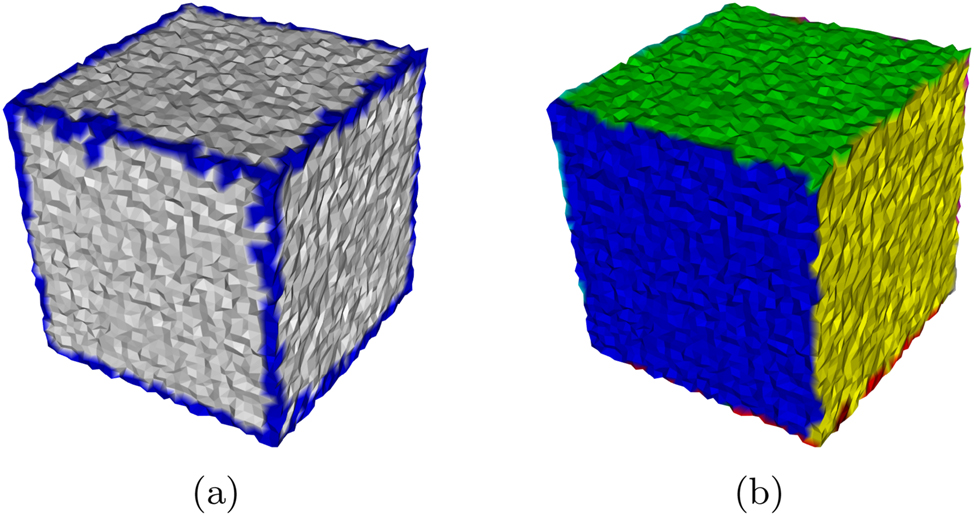
Synthetic cube with noise (a) edge detection and (b) segmentation.
6.2 Evaluation metric
To evaluate the correctness of a calculated segmentation with labels L C , we need to determine which points have been classified correctly based on the ground truth segmentation with labels L G . Hence, we calculate the intersection over union (IoU) for each ground truth label l g with each of our calculated labels l c . We then pair up labels, if the calculated label for which the ground truth label has its maximal IoU also has the ground truth label as maximal IoU, so
This guarantees, that neither taking only one label nor taking a very fine segmentation result in high scores. Then we can get the correctness of our segmentation by adding up the intersections of each pair of correctly classified labels and dividing by the total number n of vertices of the mesh
The Score thereby gives us a percentage of correctly labeled vertices.
6.3 Results on dataset
We run a pipeline for a range of parameters on each of our 62 manually annotated artifacts and compare each result with the ground truth of the same artifact. Taking the average of the best results for each artifact then gives us an estimation of the potential of our method.
Across all 62 artifacts we achieve an average of 91.26 % correctly labeled vertices in a range from 81.2 % to 97.2 %. The artifact GdF 31 in Figure 11 for example reaches 92.5 % correctly labeled vertices for the best result. Some more examples compared to their ground truths can be seen in Figure 13 where we show some good as well as bad results, including the worst Figure 13(f) and best Figure 13(b) artifacts.
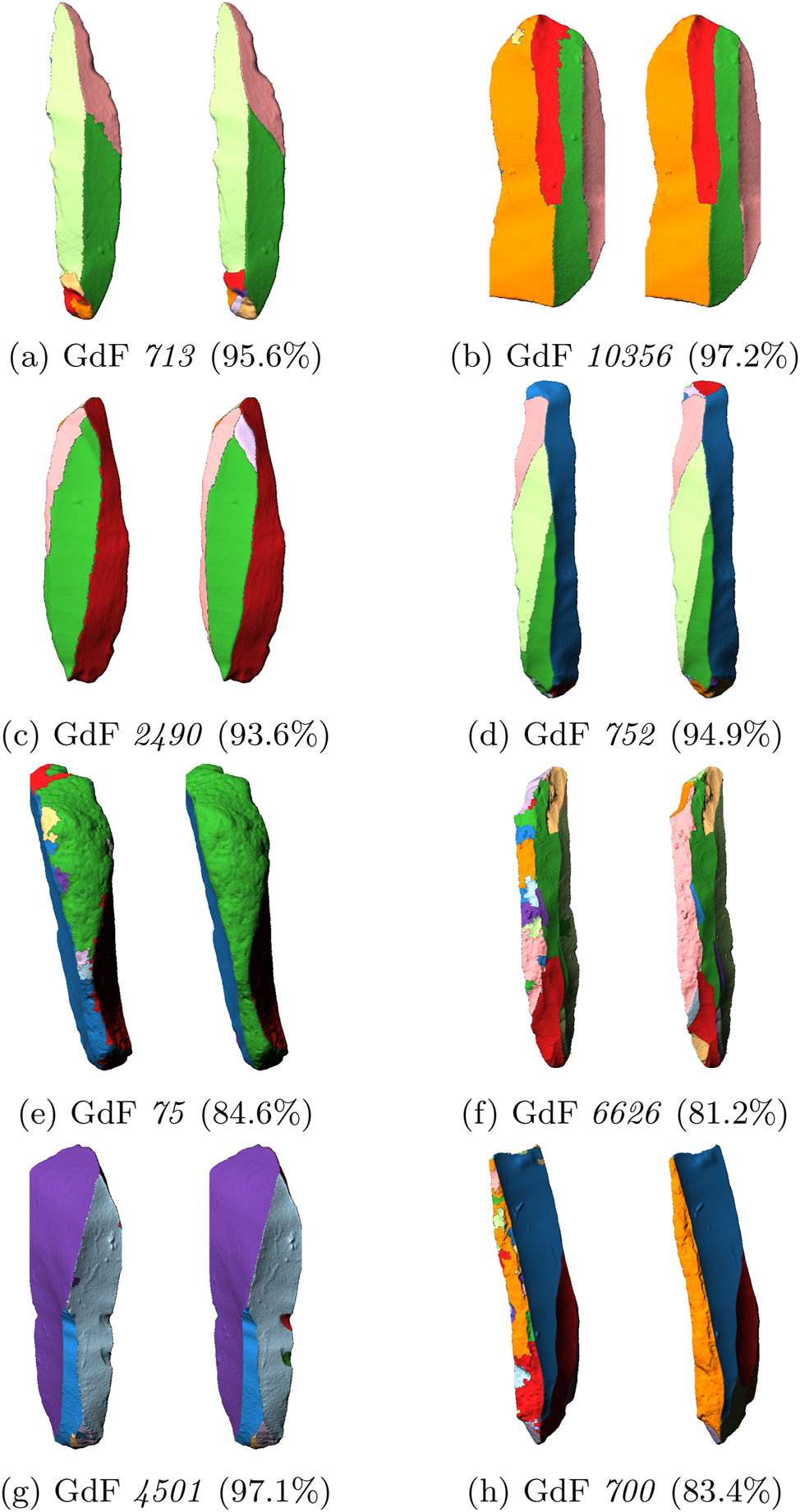
Different results (left) with ground truths (right).
Note how especially artifacts with rough unworked areas (cortex), e.g., Figure 13(e), (f), and (h) are challenging for our method, as they characteristically have a lot of high curvature values and therefore also ridges with high separatrix persistences. This leads to an oversegmentation of these areas although they should be labeled as one area. Artifacts containing such cortex areas are best pre-labeled as we show with the user-guided segmentation in Section 6.4.
Further weak scars are challenging if the curvature values along their ridges are not large enough to properly be detected. In artifact GdF 4501 Figure 13(g) for example we have two very small scars, that are not detected in the best result in terms of correctly labeled vertices as shown in Figure 15(a).
6.4 Conforming results
Taking a manual segmentation as described in 4.3 and shown in Figure 10, enables the user to achieve even better results. Since the improvement depends on the amount and quality of manual labeling that is done, we cannot quantitatively evaluate how much this improves the results without evaluating the manual pre-labeling work. Therefore we just showcase the improvement using the two masks that were created in Figure 10. Figure 14 shows the original results for the two artifacts GdF 4501 and 700 on the left (a) and (d), the conforming results using the pre-labeling in the middle (b) and (e) and the ground truth on the right (c) and (f). Note that the improvement in terms of correctly labeled vertices corresponds to the size of the area that was now manually pre-labeled.

Conforming results: (a)–(c) GdF 4501 result (97.1 %), conforming result (98.0 %) and ground truth; (d)–(f) GdF 700 result (83.4 %), conforming result (92.5 %) and ground truth.
Figure 15 highlights the two weak scars again, that were now pre-labeled, but due to their small area and consequently relatively few vertices, they only improve the segmentation result by 0.9 %.

Artifact GdF 4501 (a) result, (b) conforming result and (c) ground truth.
7 Conclusion and outlook
The segmentation of scars is a necessary step towards a more automated analysis of stone artifacts and their production steps by extracting the spatial properties of each scar area and analyzing the underlying patterns. In archaeology, a central aspect is the operational sequence (chaîne opératoire). When applied to the lithic production sequence, it describes the relative chronology of scars and determines the category of production stage to which they belong. In this manual approach, the completeness [28] and the chronological relation [29] of adjacent and overlapping scars are evaluated. These defined conditions for determining the production stages or the relative chronology are analyzed, for example, with the MSII curvature values or the roughness of the scar outlines.
To enable such an analysis on a scar level, 3D annotations are required and we now provide a method to speed up this process, such that it is possible to segment an artifact in a couple of minutes (including the time to find the correct parameters) instead of manually painting each artifact, which takes 45 min in average depending on the wanted precision and complexity of the scar pattern. To make it even easier to segment lithic artifacts, we are working on a parameter suggestion, that will try to give the user a good parameter combination depending on the properties of the artifact. Other GUI usability improvements are planned such as the ability to merge two labels in just two clicks.
Regarding our segmentation method, we are experimenting with different options especially for the first two steps: ridge detection and oversegmentation. For the oversegmentation we will test ascending manifolds of the minima as done in Ref. [14], which would still originate in Morse theory, or try a clustering approach based on the detected ridges as oversegmentation. The latter takes advantage of the intended order of application in the GUI tool, where we detect the ridges first and then perform the segmentation. Looking at the ridge detection, we are testing different fine tuning options for filtering the separatrices. Also noise removing and/or edge enhancing filters on the input curvature values could improve the ridge detection.
Introducing the user-guided segmentation method using conforming MS complexes, also enables to automatically pre-segment an artifact and use that as input for the conforming MS complexes. Especially the rough areas could be automatically determined via their surface roughness in the future. Our method now is already set up to handle such inputs.
About the authors

Jan Philipp Bullenkamp received a master in mathematics from Heidelberg University. Currently he works on Morse Smale complexes and discrete vector fields on 3D meshes as a PhD student in computer science in the eHumanities group Informatics and Cultural Heritage of Hubert Mara at Martin Luther University Halle-Wittenberg.

Theresa Kaiser received a bachelor in mathematics and recently also in computer science from Heidelberg University, Germany. She is currently working in the group Computational Arithmetic Geometry of Gebhard Böckle at the Interdisciplinary Center for Scientific Computing (IWR) on a master thesis about Drinfeld modular forms.

Florian Linsel holds a master degree in archaeology from the University of Cologne and is currently working in the eHumanities group Informatics and Cultural Heritage of Hubert Mara at the Martin Luther University Halle-Wittenberg. As a PhD student in computer science, his work focuses on the analysis of lithic artifacts with statistical methods to determine the underlying techniques.

Dr. Susanne Krömker is head of the Visualization and Numerical Geometry Group at the Interdisciplinary Center for Scientific Computing (IWR) at Heidelberg University, Germany. She received her PhD in mathematics with an application in chemistry and works as a lecturer for computer science and mathematics with a focus on computer graphics and computational geometry.

Prof. Dr. Hubert Mara received a master in computer science from Technical University Vienna, Austria, and his PhD in 2012 from Heidelberg University, Germany. As part of his doctoral thesis, he developed the GigaMesh Software Framework. He then headed the Forensic Computational Geometry Laboratory in Heidelberg until 2020 and moved to Mainz University of Applied Sciences as managing director of the Mainz Center for Digitality in the Humanities and Cultural Sciences (mainzed). Today, he is head of the eHumanities group Informatics and Cultural Heritage at Martin-Luther University Halle-Wittenberg.
-
Research ethics: Not applicable.
-
Author contributions: The authors have accepted responsibility for the entire content of this manuscript and approved its submission.
-
Competing interests: The authors state no conflict of interest.
-
Research funding: None declared.
-
Data availability: The raw data is published alongside (cited in the publication) and is publicly available.
-
Software availability: The software is published alongside (cited in the publication) and is publicly available.
References
[1] D. Angelucci, “Lithic artefacts,” in Archaeological Soil and Sediment Micromorphology, Hoboken, United States, John Wiley & Sons Ltd., 2017, pp. 223–230.10.1002/9781118941065.ch27Search in Google Scholar
[2] D. Marcazzan, C. Miller, B. Ligouis, R. Duches, N. Conard, and M. Peresani, “Middle and upper paleolithic occupations of Fumane Cave (Italy): a geoarchaeological investigation of the anthropogenic features,” J. Anthropol. Sci., vol. 101, pp. 37–62, 2022, https://doi.org/10.4436/JASS.10002.Search in Google Scholar PubMed
[3] T. Homburg, R. Zwick, H. Mara, and K. Bruhn, “Annotated 3D-models of cuneiform tablets,” J. Open Archaeol. Data, vol. 10, p. 5, 2022. https://doi.org/10.5334/joad.92.Search in Google Scholar
[4] L. Herzlinger and L. Grosman, “AGMT3-D: a software for 3-D landmarks-based geometric morphometric shape analysis of archaeological artifacts,” PLoS One, vol. 13, no. 11, pp. 1–17, 2018. https://doi.org/10.1371/journal.pone.0207890.Search in Google Scholar PubMed PubMed Central
[5] Grosman, et al., “Artifact3-D: new software for accurate, objective and efficient 3D analysis and documentation of archaeological artifacts,” PLoS One, vol. 17, no. 6, pp. 1–24, 2022. https://doi.org/10.1371/journal.pone.0268401.Search in Google Scholar PubMed PubMed Central
[6] J. O. Figueroa, J. Reeves, S. McPherron, and C. Tennie, “A proof of concept for machine learning-based virtual knapping using neural networks,” Sci. Rep., vol. 11, no. 1, pp. 1–12, 2021. https://doi.org/10.1038/s41598-021-98755-6.Search in Google Scholar PubMed PubMed Central
[7] J. Gellis, C. Smith, and R. Foley, “PyLithics: a python package for stone tool analysis,” J. Open Source Softw., vol. 7, no. 69, p. 3738, 2022. https://doi.org/10.21105/joss.03738.Search in Google Scholar
[8] E. Richardson, L. Grosman, U. Smilansky, and M. Werman, “Extracting scar and ridge features from 3D-scanned lithic artifacts,” in Archaeology in the Digital Era: 40th Annual Conference of Computer Applications and Quantitative Methods in Archaeology (CAA), 2014, pp. 83–92.10.1017/9789048519590.010Search in Google Scholar
[9] J. Milnor, M. Spivak, and R. Wells, Morse Theory. (AM-51), vol. 51, Princeton University Press, 1969. Available at: http://www.jstor.org/stable/j.ctv3f8rb6.Search in Google Scholar
[10] R. Forman, “A user’s guide to discrete Morse theory,” Séminaire Lothar. Comb., vol. 48, p. B48c–B35, 2001.Search in Google Scholar
[11] D. Günther, A. Jacobson, J. Reininghaus, H. P. Seidel, O. Sorkine-hornung, and T. Weinkauf, “Fast and memory-efficient topological denoising of 2D and 3D scalar fields,” IEEE Trans. Visual. Comput. Graph., vol. 20, no. 12, pp. 2585–2594, 2014. https://doi.org/10.1109/tvcg.2014.2346432.Search in Google Scholar PubMed
[12] V. Robins, P. Wood, and A. Sheppard, “Theory and algorithms for constructing discrete Morse complexes from grayscale digital images,” IEEE Trans. Pattern Anal. Mach. Intell., vol. 33, no. 8, pp. 1646–1658, 2011. https://doi.org/10.1109/tpami.2011.95.Search in Google Scholar
[13] L. De Floriani, U. Fugacci, F. Iuricich, and P. Magillo, “Morse complexes for shape segmentation and homological analysis: discrete models and algorithms,” Comput. Graph. Forum, vol. 34, no. 2, pp. 761–785, 2015. https://doi.org/10.1111/cgf.12596.Search in Google Scholar
[14] X. Xu, F. Iuricich, K. Calders, J. Armston, and L. De Floriani, “Topology-based individual tree segmentation for automated processing of terrestrial laser scanning point clouds,” Int. J. Appl. Earth Obs. Geoinf., vol. 116, p. 103145, 2023. https://doi.org/10.1016/j.jag.2022.103145.Search in Google Scholar
[15] H. Mara and S. Krömker, “Vectorization of 3D-characters by integral invariant filtering of high-resolution triangular meshes,” in 2013 12th International Conference on Document Analysis and Recognition, 2013, pp. 62–66.10.1109/ICDAR.2013.21Search in Google Scholar
[16] A. Falcucci and M. Peresani, The Open Aurignacian Project. Volume 1: Fumane Cave in Northeastern Italy, Geneva, Switzerland, Zenodo, 2022.Search in Google Scholar
[17] T. Higham, F. Brock, M. Peresani, A. Broglio, R. Wood, and K. Douka, “Problems with radiocarbon dating the middle to upper palaeolithic transition in Italy,” Quat. Sci. Rev., vol. 28, no. 13–14, pp. 1257–1267, 2009. https://doi.org/10.1016/j.quascirev.2008.12.018.Search in Google Scholar
[18] A. Marin-Arroyo, G. Terlato, M. Vidal-Cordasco, and M. Peresani, “Subsistence of early anatomically modern humans in Europe as evidenced in the protoaurignacian occupations of Fumane Cave, Italy,” Sci. Rep., vol. 13, no. 1, p. 3788, 2023. https://doi.org/10.1038/s41598-023-30059-3.Search in Google Scholar PubMed PubMed Central
[19] H. Edelsbrunner, D. Letscher, and A. Zomorodian, “Topological persistence and simplification,” in Proceedings 41st Annual Symposium on Foundations of Computer Science, 2000, pp. 454–463.Search in Google Scholar
[20] A. Gyulassy, D. Günther, J. Levine, J. Tierny, and V. Pascucci, “Conforming Morse-Smale complexes,” IEEE Trans. Visual. Comput. Graph., vol. 20, no. 12, pp. 2595–2603, 2014. https://doi.org/10.1109/tvcg.2014.2346434.Search in Google Scholar
[21] T. Weinkauf and D. Günther, “Separatrix persistence: extraction of salient edges on surfaces using topological methods,” Comput. Graph. Forum, vol. 28, no. 5, pp. 1519–1528, 2009. https://doi.org/10.1111/j.1467-8659.2009.01528.x.Search in Google Scholar
[22] J. Bullenkamp, T. Häberle, and H. Mara, MorseMesh, Geneva, Switzerland, Zenodo, 2023.Search in Google Scholar
[23] M. Falcucci and M. Peresani, “The contribution of integrated 3D model analysis to Protoaurignacian stone tool design,” PLoS One, vol. 17, no. 5, pp. 1–29, 2022. https://doi.org/10.1371/journal.pone.0268539.Search in Google Scholar PubMed PubMed Central
[24] N. Conard and M. Bolus, “Chronicling modern human’s arrival in Europe,” Science, vol. 348, no. 6236, pp. 754–756, 2015. https://doi.org/10.1126/science.aab0234.Search in Google Scholar PubMed
[25] J. Hublin, “The modern human colonization of Western Eurasia: when and where?,” Quat. Sci. Rev., vol. 118, pp. 194–210, 2015. https://doi.org/10.1016/j.quascirev.2014.08.011.Search in Google Scholar
[26] P. Cignoni, M. Callieri, M. Corsini, M. Dellepiane, F. Ganovelli, and G. Ranzuglia, “MeshLab: an open-source mesh processing tool,” in Eurographics Italian Chapter Conference, 2008, pp. 129–136.Search in Google Scholar
[27] F. Linsel, J. Bullenkamp, and H. Mara, 3D Data Derivatives of Grotta di Fumane: GigaMesh-Processed, Annotations and Segmentations, Geneva, Switzerland, Zenodo, 2023.Search in Google Scholar
[28] J. Richter, “Copies of flakes: operational sequences of foliate pieces from Buran-Kaya III level B1,” in The Middle Paleolithic and Early Upper Paleolithic of Eastern Crimea, 2004, pp. 233–247.Search in Google Scholar
[29] A. Pastoors, Y. Tafelmaier, and G. Weniger, “Quantification of late pleistocene core configurations: application of the working stage Analysis as estimation method for technological behavioural efficiency,” Quartär, vol. 62, no. 1, pp. 63–84, 2015.Search in Google Scholar
© 2024 the author(s), published by De Gruyter, Berlin/Boston
This work is licensed under the Creative Commons Attribution 4.0 International License.
Articles in the same Issue
- Frontmatter
- Editorial
- Kleine Fächer Digital
- Research Articles
- Discrete Morse theory segmentation on high-resolution 3D lithic artifacts
- Signed, sealed, delivered – digital approaches to Byzantine sigillography
- Matschoss 2.0 - Virtual machine collections as the missing link between museums and historic monuments
- A recursive encoding for cuneiform signs
- A case study of the use of logical data analysis in the Workmen’s Village in Tell el-Amarna, Egypt
- Digital and computational archaeology in Germany