Calendering of thermoplastics: models and computations

1 Introduction

Calendering is a process used in a wide variety of industries for the production of rolled sheets or films of specific thickness and final appearance. The procedure has been theoretically introduced more than 50 years ago (Gaskell 1950) and involves the feed from an infinite reservoir of a pair of co-rotating heated rolls (calenders) with a material to form a sheet. The case of calendering fed with a finite sheet of thickness H _f for the production of a final sheet with exit thickness H, as shown in Figure 1 (Middleman 1977), is a variant of the process. In calendering, the ratio of the calender radius to the distance between calenders (gap) should be significantly higher than 1, that is, R/H ₀ >> 1 [O(1000)].

Figure 1:

Schematic representation of the calendering process with a finite sheet. The sheet thickness is reduced from 2H _f to 2H. The minimum gap is 2H ₀, and the roll radius is R, with R/H ₀ ≈ 1000.

The quality of the sheet or film produced is determined by the flow and heat transfer phenomena in the gap between the two rotating rolls. It is thus of great importance to determine the velocity and temperature profiles as the melt is squeezed between the rolls, the pressure distribution on the roll surfaces, the roll-separating force, the torque and energy input. A realistic Newtonian and Bingham flow analysis by Gaskell (1950) spearheaded further developments in modelling. McKelvey (1972) reworked Gaskell’s model for Newtonian flow and extended it to include non-Newtonian (i.e. shear-thinning) effects.

JV’s first encounter with calendering occurred during his first sabbatical leave in 1974 in Germany, where some inaccuracies in McKelvey’s (1972) power consumption calculations were corrected by Ehrmann and Vlachopoulos (1975). The problem was then taken in earnest by Kiparissides and Vlachopoulos (1976), who developed a finite element analysis for symmetric and asymmetric calendering (different roll speeds, different roll diameters). Viscous dissipation effects were included in the finite difference solutions of the energy equation by Kiparissides and Vlachopoulos (1978). An isothermal model with slip was developed by Vlachopoulos and Hrymak (1980) using the lubrication approximation and a Runge-Kutta solution.

The vast majority of the above works is based on the Lubrication Approximation Theory (LAT) of Reynolds. The textbook by Middleman (1977) nicely summarizes this and presents the most important findings up to 1977. Lifting this approximate assumption leads to a truly two-dimensional (2-D) analysis, as was done by Mitsoulis et al. (1985) and Agassant and Espy (1985). They have shown very interesting results with intricate patterns dominated by large vortices in the melt bank before the rolls. Zheng and Tanner (1988) also solved the 2-D problem for Newtonian, power-law and viscoelastic fluids, with particular emphasis on finding the point where the fluid detaches from the rolls. They used a boundary element method and the criterion that the fluid detaches from the rolls at the point where the tangential traction becomes zero. Again, all reports prior to 1990 have been summarized in the textbook by Agassant et al. (1991). More recently, Levine et al. (2002) used a 2½-D approach to calculate the side spreading of the calendered sheet while employing the lubrication approximation for the flow through the nip. Mewes et al. (2002) have done work on the simultaneous calculation of roll deformation and polymer flow, while the full three-dimensional (3-D) problem has been solved by Luther and Mewes (2004) and Polychronopoulos et al. (2014) for Newtonian and power-law fluids. Note also the paper by Magnier et al. (2013) devoted to non-symmetrical calendering, which provides analytical LAT calculations and comparison with experiments. A new version of the 1991 textbook by Agassant et al. (1991) has been published in 2017 with more advanced developments on the calendering process (Chapters 8 and 10, paragraph 3) (Agassant et al. 2017).

A renewed effort has appeared recently to study viscoplastic materials in calendering and find out the effect of yield stress. A series of papers by Sofou and Mitsoulis (2004a, 2004b, 2006 have used LAT and carried out full parametric studies for pseudoplastic and viscoplastic fluids obeying the Herschel-Bulkley model of viscoplasticity with or without slip at the wall. This model, upon appropriate simplifications, can be reduced to the Newtonian, power-law and Bingham plastic models. The results have shown interesting trends and yielded/unyielded regions. However, the latter are misleading as pointed out by Sofou and Mitsoulis (2004a), and by Mitsoulis (2008) who used a fully 2-D analysis, and they are a direct consequence of using LAT and its inherent approximations.

It is, therefore, the purpose of the present paper to review the problem of calendering, to present the major results so far and to show new ones from time-dependent calculations. Some issues, which still remain unresolved, will be discussed for future work.

2 Mathematical modeling

The problem at hand is shown schematically in Figure 1, where a fluid is squeezed between two rotating rolls moving with a roll speed, U, and exits with a reduced thickness, 2H, which is unknown a priori.

Many materials used in calendering are non-Newtonian, exhibiting either pseudoplastic (shear–thinning or –thickening) or viscoplastic (presence of a yield stress) or viscoelastoplastic behavior (see, e.g., Bird et al. (1983)). Models describing pseudoplastic behavior include the power-law, Carreau, Cross, and others. Models describing viscoplastic behavior include the Bingham, Herschel-Bulkley and Casson. Models describing viscoelastoplastic behavior include the K-BKZ and Phan-Thien/Tanner (PPT) models.

The Herschel-Bulkley model has the advantage of reducing – with an appropriate choice of parameters – to the Bingham, power-law or Newtonian models. In simple shear flow (1-D) it becomes:

where τ is the shear stress, γ ˙ is the shear rate, τ _y is the yield stress, K is the consistency index, and n is the power-law index. Note that when n = 1 and K = ɳ (a constant), the Herschel-Bulkley model reduces to the Bingham model. When τ _y  = 0, the power-law model is recovered, and when τ _y  = 0 and n = 1, the Newtonian model is obtained.

It should be noted that in viscoplastic models, when the shear stress τ falls below τ _y , a solid structure is formed (unyielded). Also in viscoplasticity, a dimensionless yield stress can be defined by:

where H ₀ is a characteristic length (half the minimum gap between the rolls), (dP/dx)₀ is a pressure gradient evaluated at the nip, and y ₀ is a yield line separating the yielded from the unyielded material. In all cases, the Newtonian fluid corresponds to τ _y * = 0. However, at the other extreme of an unyielded solid, τ _y * → 1, a limiting value, where the material becomes all unyielded.

If the dimensionless yield stress is based on the kinematics through the roll speed U, it gives rise to the Bingham number, Bn, defined by:

Again, the Newtonian fluid corresponds to Bn = 0. However, at the other extreme of an unyielded solid, Bn → ∞.

The flow is governed by the usual conservation equations of mass and momentum under isothermal creeping flow conditions for an incompressible viscous fluid. The constitutive equation that relates the stresses to the velocity gradients is the generalized Newtonian fluid. In full tensorial form the constitutive equation is written as:

where η is the apparent viscosity given for the Herschel-Bulkley-Papanastasiou model by

and | γ ˙ | is the magnitude of the rate-of-strain tensor γ ˙ ‾ ‾ = ∇ v ‾ + ∇ v ‾ T , which is given by

where II γ ˙ is the second invariant of γ ˙ ‾ ‾ .

The stress growth exponent m is the regularization parameter introduced by Papanastasiou (1987), and it has to be high enough to approximate the ideal viscoplastic model (Mitsoulis et al. 1993; Papanastasiou 1987). The dimensionless form of Eq. (5) is written as

where the dimensionless stress growth exponent M is given by

As in our previous works (Mitsoulis et al. 1993; Papanastasiou 1987), to track down yielded/unyielded regions, we shall define yielded and unyielded fluid regions by the following criteria:

In parametric studies for pseudoplastic models obeying the power law, the dimensionless parameter is the power-law index, n. For viscoplastic models obeying the Bingham model, the dimensionless parameter is the Bingham number, Bn. In the present simulations, the range of parameters is 0 ≤ n ≤ 2, and 0 ≤ Bn ≤ 1000.

3 Governing equations (LAT)

LAT considers locally fully developed shear flow between the rolls. The conservation of momentum equation then gives

where τ _xy  = τ is the shear stress in the transverse direction. The shear stress is given by the Herschel-Bulkley model in the present work, i.e. Eq. (1).

It should be noted that LAT is not strictly applicable to yield stress materials as the material velocity in the unyielded area at abscissa x will be different from the material velocity in the unyielded area at abscissa (x + dx). This is solved artificially by a regularization technique (Eq. (5)) but leads to tricky results. When Bn becomes infinite, which corresponds to a rigid plastic behavior, this is solved in the steel rolling models by imposing a slip velocity, which is varying along the contact with the rolls.

We integrate Eq. (10) and apply the boundary conditions for symmetric calendering, i.e.

From the mathematical analysis, we know that there are two flow regions in the x-direction, one region near the nip and the exit, which has a negative pressure gradient and a negative velocity gradient, and another region away from the nip at the entrance with opposite signs. For viscoplastic materials, we know that there are also two flow regions in the y-direction, one where the material is unyielded (y ≤ y ₀) and another where it is yielded (y > y ₀). We also note that τ y = | d P / d x | y 0 . Thus, we obtain:

Integration of the velocity profile gives the volumetric flow rate Q according to:

In the case of the Bingham plastic model (n = 1), the above equation becomes:

From Eq. (12) the pressure gradient dP/dx can be found. The following dimensionless parameters are introduced (Middleman 1977):

where λ is a dimensionless flow rate (or leave-off distance) and the rest of the symbols are defined in Figure 1. After the appropriate manipulations, the following dimensionless pressure gradient is obtained:

Equation (16) incorporates both cases: for −∞ < x′ < −λ the pressure gradient is positive, and for −λ ≤ x′ ≤ λ the pressure gradient is negative. Integration of the above Eq. (16) requires boundary conditions for the pressure gradient dP′/dx′ and the pressure P′ as well. In the case of an infinite reservoir, the standard conditions are the so-called Swift conditions (Zheng and Tanner 1988):

Then the pressure is given by the integral:

The extrema of the pressure distribution occur at x = −∞, ±λ _∞. The dimensionless leave-off distance λ _∞ corresponding to an infinite reservoir can be found from the above equation knowing that P ′ ( x ′ = − ∞ ) = 0 . Therefore, λ _∞ can be found from the relation:

The above integral has no analytical solution for the general case of Herschel-Bulkley fluids. Therefore, a numerical solution of the non-linear equations must be found.

4 Results and discussion

The first paper by Ehrmann and Vlachopoulos (1975) showed that small numerical errors in the attachment point −x _f * caused large errors in the power consumption. This becomes evident in Figure 2, where the original figure from Ehrmann and Vlachopoulos (1975) is presented and it gives the correction to the coefficient f related to the power input (Eq. (26a)) as a function of the leave-off distance λ. This attention to detail established a genuine feel for the process of calendering, and what the numbers meant in meaningful calculations.

Figure 2:

Correction of the power consumption coefficient f as a function of the leave-off distance λ as found out by Ehrmann and Vlachopoulos (1975) for calendering of Newtonian fluids.

The subsequent work by Kiparissides and Vlachopoulos (1976) used the finite element method (FEM) to study the process. The original FEM grid from the computations is shown in Figure 3 and consists of 64 triangular elements and 157 nodes. Such grids at the time (1976) were only allowed due to memory limitations of the mainframe computers. The results for the pressure for Newtonian fluids showed that they were in good agreement with LAT only for low values of λ ≤ 0.3, as shown in Figure 4. This was due to the fact that although the grid was 2-D, only one velocity component u _x was used in the calculations due to memory limitations. Further results on non-isothermal calendering (Kiparissides and Vlachopoulos 1978) took into account the viscous dissipation term in the energy equation and showed interesting non-monotonic temperature profiles close to the walls for the first time (Figure 5).

Figure 3:

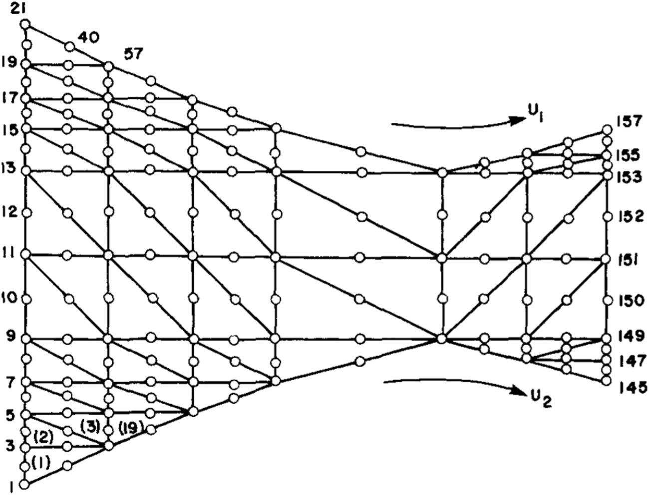
Finite element grid for asymmetric calendering (Kiparissides and Vlachopoulos 1976). The grid consists of 64 triangular elements and 157 nodes.

Figure 4:

Pressure distribution as a function of the dimensionless distance ρ = x’ in calendering of Newtonian fluids (Kiparissides and Vlachopoulos 1976).

Figure 5:

Temperature development along the flow field in calendering of Newtonian fluids (Kiparissides and Vlachopoulos 1978).

JV’s subsequent work was with Andy Hrymak (then an undergraduate student at McMaster University). The task was to simulate experimental data for a rigid PVC compound known to exhibit slip at the wall. In a landmark paper (Vlachopoulos and Hrymak 1980), the equations for power-law fluids were recast with slip and solved for with a 4th-order Runge-Kutta method, giving the results of Figure 6 (continuous lines), which were later verified by the author with a full 2-D FEM solution (symbols) (Mitsoulis et al. 1985). The paper by Vlachopoulos and Hrymak (1980) was the only paper at the time that had comprehensive experimental data both for the resin and the process. It remains to this date perhaps the only well documented paper with experiments on calendering. Agassant and Philippe (1983) have compared experimental and computed roll separating forces and calendering torques.

Figure 6:

Pressure distribution as a function of dimensionless distance taking into account slip at the wall for a rigid PVC melt. Continuous lines are from (Vlachopoulos and Hrymak 1980) with LAT, symbols are 2-D FEM results from Mitsoulis et al. (1985).

The full 2-D problem was first tackled by the main author, then working as a graduate student for his PhD with JV, in Mitsoulis et al. (1985). JV’s inspiration and guidance were unique in getting results for a fully 2-D, non-isothermal, pseudoplastic or viscoelastic FEM analysis with slip at the wall, and the determination of the free surface in the melt bank that had defied description up to that time. Results from that work appeared in 1985 in Polymer Engineering and Science (Mitsoulis et al. 1985). Reproduced here are the FEM grids for the velocities-pressure (u-v-p formulation) (Figure 7A), the temperature (T) and stream function (ψ) solution (Figure 7B). The results for the streamlines and isotherms are shown in Figure 8A,B, respectively. They showed for the first time the intricate patterns observed experimentally by Agassant and Espy (1985) (Figure 9). Note that Agassant and Espy (1985) developed also a FEM computation based on streamline and vorticity functions.

Figure 7:

Finite element grids for calendering of PVC with determination of the free surface upstream in the melt bank, A) u-v-p grid, B) T-ψ grid (Mitsoulis et al. 1985).

Figure 8:

Results from the 2-D analysis for calendering of PVC with determination of the free surface upstream in the melt bank, A) streamlines, B) isotherms (Mitsoulis et al. 1985).

Figure 9:

Experimental results from calendering rigid PVC (Agassant and Espy 1985).

When looking at successive slices of the upstream polymer bank (reservoir) in non-stationary conditions, one observes that the lower recirculation (see Figures 8 and 9) gradually surrounds the upper one. When it comes into contact with the upper roll there is a kinematic incompatibility, which splits this recirculating cell into two parts leading to a third recirculating cell (see Agassant et al. 2017, chapter 10.3), which is at the origin of the so-called V-shaped defects in the calendered sheet.

The 2-D results remained for a long time without any improvement or addition in the literature, as they seemed to have answered the major points of analysis in calendering. Viscoelastic results by Zheng and Tanner (1988) (Figure 10) showed that viscoelasticity did not alter the results appreciably, as also found earlier in Mitsoulis et al. (1985). However, that work pointed to an important issue, namely that of finding both detachment and attachment points without using the Swift condition (pressure and its derivative vanish at the detachment point, Eq. (18)). Instead, a method of determining the separation point numerically using the criterion of zero tangential traction was successfully applied.

Figure 10:

The effect of viscoelasticity on the pressure distribution in calendering of a Newtonian fluid (dashed line) and a viscoelastic fluid obeying the PTT model at Weissenberg number Ws = 1 (Zheng and Tanner 1988).

It was only in the 2000’s that new additions were made in the literature. They started with a 2½-D approach to calculate the side spreading of the calendered sheet while employing the lubrication approximation for the flow through the nip (Levine et al. 2002). Typical results are shown in Figure 11, where spreading of the sheet is more pronounced for a ratio W ₀/H ₀ = 10 than for a ratio W ₀/H ₀ = 60, where W ₀ is the incoming sheet width.

Figure 11:

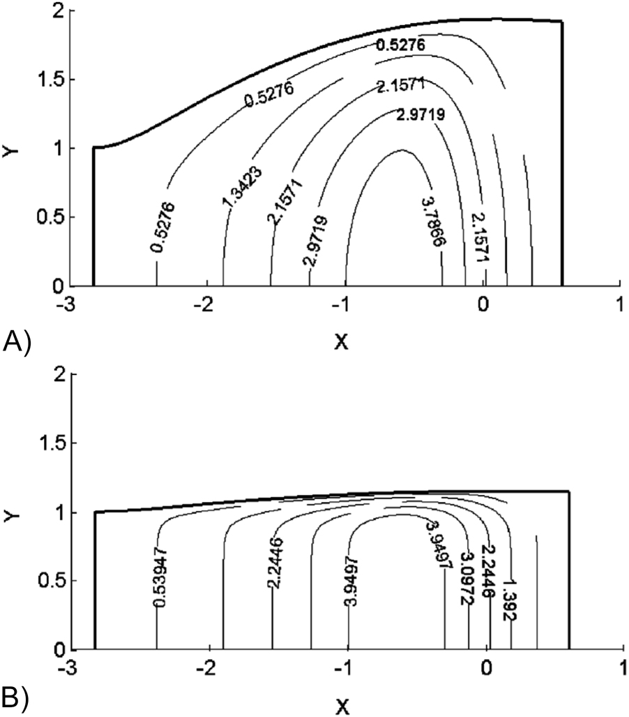
Shape and pressure contours in calendering analysis of spreading sheets (2½-D approach), A) W ₀/H ₀ = 10, B) W ₀/H ₀ = 60 (Levine et al. 2002).

The first experimental observations on the three-dimensional (3D) effects in calendering were carried out by Unkrüer (1970), using PVC and PS. His conclusions were that (i) the calendered sheet spreads, (ii) three vortices are formed in and near the melt bank, and (iii) the material is conveyed from the melt bank to the sides through a spiraling flow pattern (see Figure 12A). He also observed and measured a pressure drop along the cylinder axis of symmetry (transverse direction).

Figure 12:

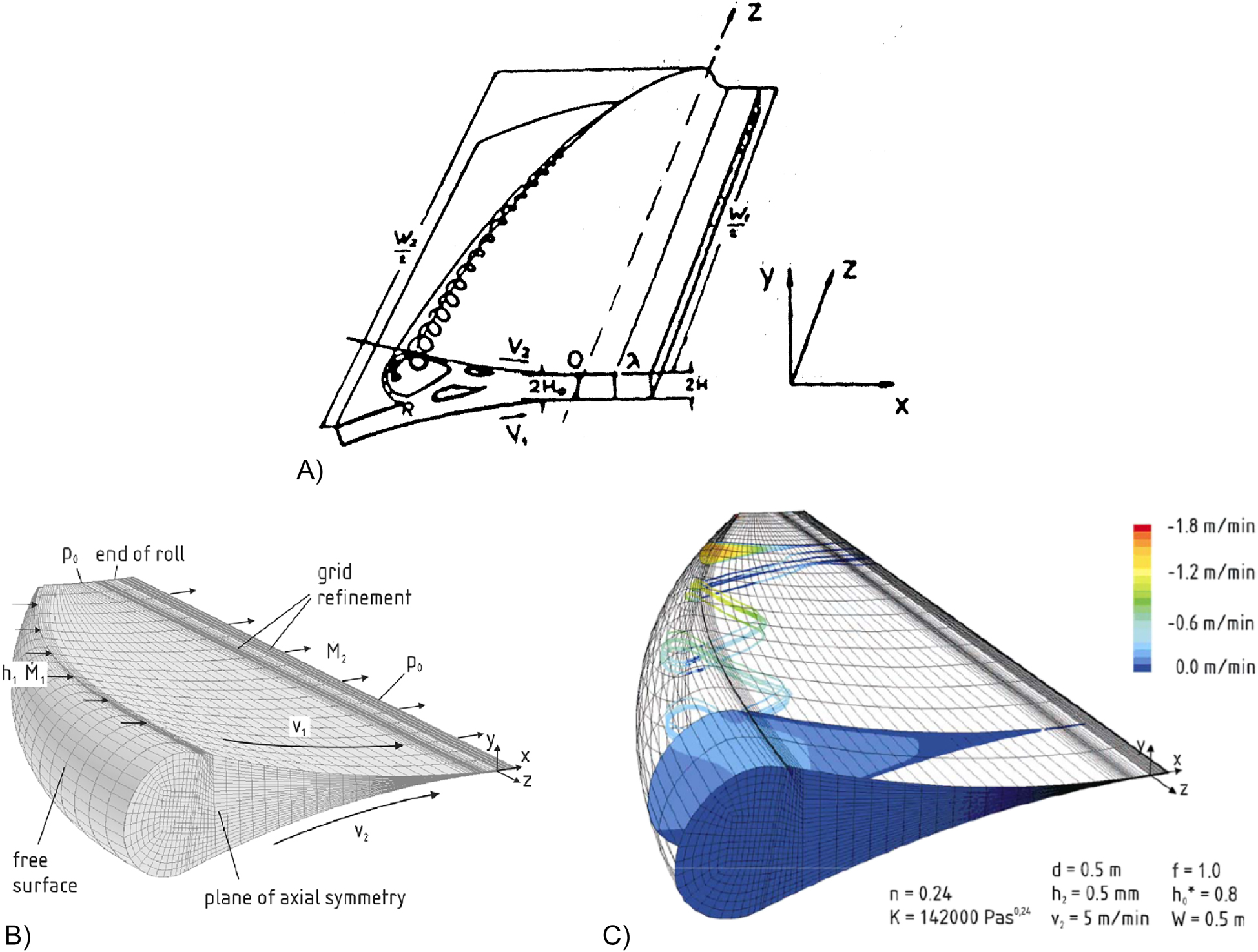
Schematic spiral motion view from Unkrüer (1970) (A). 3-D computations of calendering power-law fluids, B) FEM grid, C) velocity field showing a spiral motion in the 3rd-direction (Luther and Mewes 2004).

Modeling the 3D flow patterns in calendering has been very limited. The first full three-dimensional (3-D) problem for power-law fluids was tackled by Luther and Mewes (2004), who used the commercial package POLYFLOW^® and computed the upstream free surface in its full length. The results are indeed very impressive and exciting, as evidenced in Figure 12. They reveal the three-dimensional spiral motion in the melt bank and a bending of the upstream free surface to accommodate a melt bank that is thickest at the middle and thinnest towards the ends of the rolls. However, predictions for the sheet spreading and existence of transverse pressure profiles were not included by the authors. If any criticism is made for an otherwise tremendous piece of work, it involves the difficulty of the solution, the lack of any information of how this was achieved (except that it was difficult), and the inability to reproduce these results by somebody else.

A more tractable 3D numerical approach has been carried out by Polychronopoulos et al. (2014) for Newtonian and power-law materials, using the OpenFOAM software (based on the Finite Volume Method – FVM). In their study, the material was assumed to be fed in the form of a thick sheet with finite width. A decoupled iterative numerical procedure was used to determine the shape of the side spreading free surfaces. The computational domain for the converged side free surfaces is shown in Figure 13A. The pressure distribution at the mid-plane is shown in Figure 13B and the pressure distribution at three different locations along the cylinder axis is shown in Figure 13C. The spiraling flow pattern of the molten material from the mid-width of the feed region (line AB) to one of spreading sides is shown in Figure 13D. Figure 13E shows the material rearrangement from the feed section to the sheet exit. The above numerical results are in overall agreement with the experimental observations by Unkrüer (1970) (see also Figure 12A).

Figure 13:

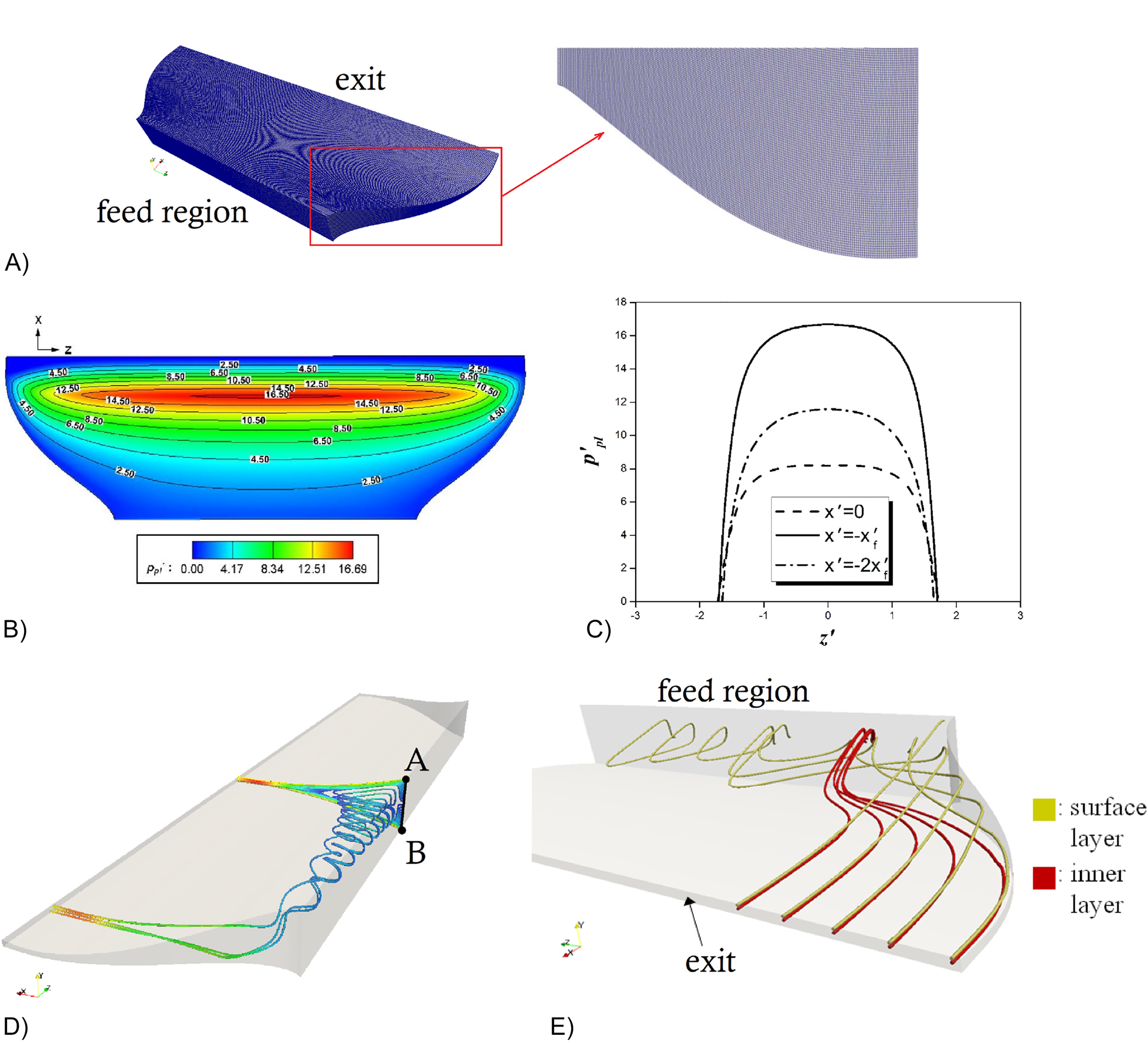
3-D numerical simulations for calendering of a power-law fluid (K = 5 × 10⁴ Pa s^0.35, n = 0.35), A) FVM grid and detail near one of the side free-surfaces, B) dimensionless pressure field on the mid-plane, C) dimensionless pressure profiles at three locations along the cylinders axis, D) spiraling flow from line AB to the side, E) material rearrangement from the feed region to sheet exit (Polychronopoulos et al. 2014).

It should be mentioned that both 3D numerical investigations by Luther and Mewes (2004) and Polychronopoulos et al. (2014) predict two vortices in the melt bank or generally in the feed section. The experiments by Unkrüer (1970) reveal the presence of a third vortex which is associated to unsteady flow phenomena. This is also evident in the experiments by Agassant and Espy (1985). Modeling the spiraling motion of all three vortices (with either the presence of a forming melt bank or a thick feeding sheet) has not yet been taken into consideration. This could be partially attributed to the complexity of the 3D flow fluid that would require a very fine (and possibly unstructured) mesh for the third vortex, combined with determination of complex-shaped free surfaces. The mathematical complexity and computational cost significantly increase if one takes into consideration the possible viscoelastic or visco-plastic nature for some materials. Therefore, complete modeling of calendering is still an open issue and more remains to be done.

4.1 Viscoplastic fluids

Starting in 2004 and in a series of papers, Sofou and Mitsoulis (2004a, 2004b, 2006) examined the effect of viscoplasticity in calendering in full parametric studies of the power-law index, n, and the Bingham number, Bn. They used LAT and the equations presented above (Eqs. (12)–(26)) to obtain solutions for three distinct cases: (a) feed from an infinite reservoir (Sofou and Mitsoulis 2004b), (b) feed with a finite sheet (Sofou and Mitsoulis 2004a), (c) both cases with slip at the wall (Mitsoulis and Sofou 2006). Typical results for the pressure distribution of Bingham fluids is shown in Figure 14, where viscoplasticity sharpens the pressure distributions and extends the flow domain.

Figure 14:

Axial distribution of dimensionless pressure for different values of the Bingham number Bn for viscoplastic fluids obeying the Bingham model (λ = 0.3) (Sofou and Mitsoulis 2004a).

Figure 15 shows the progressive growth of yielded/unyielded regions for different Bn numbers and λ = 0.3. For Bn = 0, we have purely viscous flow and the area is all yielded. At the other extreme, for Bn→∞, we have a purely plastic solid, and the area is all unyielded. Any other value of Bn between 0 and ∞ gives both yielded and unyielded regions. For the finite-sheet case shown in Figure 15, the abrupt change of the unyielded region at the point of contact is due to the limitations of the lubrication approximation, which is not valid there. These results, although interesting and exciting, are erroneous because of the limitations of LAT for viscoplastic flows (Sofou and Mitsoulis 2004a,b), namely the ever-changing geometry in the flow field (presence of non-zero velocity gradients) does not allow for unyielded regions under the gap. However, LAT is good at giving the correct pressures (Figure 14) and the sheet thicknesses, as shown in Figure 16.

Figure 15:

Progressive growth of the unyielded zones as the dimensionless Bingham number Bn increases in calendering of viscoplastic materials obeying the Bingham plastic model. The shaded regions are unyielded. The exiting sheet thickness is fixed so that λ = 0.3 (Sofou and Mitsoulis 2004a).

Figure 16:

Leave-off distance λ as a function of the entry thickness H _f /H ₀ for viscoplastic fluids obeying the Bingham model for various values of Bn (Sofou and Mitsoulis 2004a).

The results of Figure 16 have been obtained for a wide range of entering sheet thickness ratios H _f /H ₀, from the limiting case of H _f /H ₀ = 1 (no thickness reduction) to the case of H _f /H ₀ = 1000 (approaching a sheet coming from an infinite reservoir). For Bingham plastics, the results for the sheet thickness H/H ₀ are obtained for various Bn values. The Newtonian values (for Bn = 0) of λ _∞ = 0.475 and H/H ₀ = 1.226, corresponding to calendering from an infinite reservoir, are also obtained when H _f /H ₀ = 1000, as expected. Figure 16 shows that for Newtonian fluids these values are attained for H _f /H ₀ ≥ 20, while Bingham plastics, like shear-thinning fluids, require even higher ratios as the degree of viscoplasticity increases (e.g., for Bn = 1000, H _f /H ₀ = 1000 is not enough to attain the asymptotic values). It is interesting to note that for a certain value of H _f /H ₀ ≈ 15.85, the results do not depend on the Bn value (crossover points of Figure 16). The corresponding values are λ = 0.470 and H/H ₀ = 1.221. After this point, viscoplasticity increases the values. Thus, as was also the case with pseudoplastic fluids [2], it is no longer correct to say, without qualification, that the effect of non-Newtonian behavior is to increase the sheet thickness.

2-D calculations have been pursued for viscoplastic fluids, obeying the Bingham-Papanastasiou model (Eq. 7 with n = 1 and M = 1000) in a range of Bingham numbers Bn (0 ≤ Bn ≤ 1000). The extra feature in viscoplastic materials is the division of the flow field in yielded/unyielded regions by applying the criterion (9). Typical results from the simulations are shown in Figures 17 and 18 (blown-up version of Figure 17).

Figure 17:

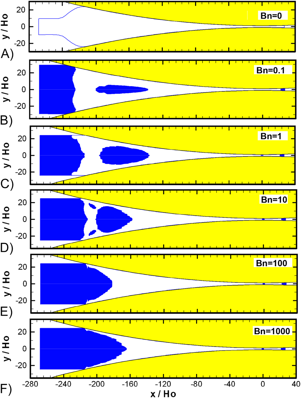
Yielded/unyielded regions as a function of the Bingham number Bn for viscoplastic fluids obeying the Bingham-Papanastasiou model with M = 1000 (Mitsoulis 2008).

Figure 18:

Blown-up section of Figure 17 under the nip in calendering of viscoplastic fluids obeying the Bingham-Papanastasiou model with M = 1000 (Mitsoulis 2008).

Increasing the Bn number leads to a monotonic increase of the unyielded region (shaded solid dark). The yielded/unyielded regions are very interesting as shown in Figure 17 for the whole flow field, and in blow-up in Figure 18 near the nip region and exit. Most of the unyielded zones are evidenced in the entering and exiting sheets, which move as rigid plugs with a constant velocity (incidentally not the roll speed U). Unlike LAT predictions, the vast areas between the rolls are yielded, and only small unyielded islands appear in the nip around the centreline. However, the pressure distributions are not that much different from LAT and as such are not shown here. Hence, all other engineering quantities are well predicted by LAT.

4.2 Time-dependent simulations

Time-dependent numerical simulations for Newtonian and viscoplastic fluids were undertaken using the Arbitrary Lagrangian-Eulerian (ALE) formulation for moving free-boundary problems (Alexandrou and Mitsoulis 2007; Hirt et al. 1974; Mitsoulis and Alexandrou 2009). Note that Serrat et al. (2012) developed the same transitory ALE computation. The reasoning behind it was that time-dependent simulations could provide the attachment and detachment points as part of the solution, as the free surface is allowed to move to accommodate the incoming and outgoing sheet.

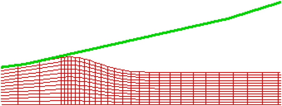
Typical results during the time evolution are shown in Figure 19 for a Newtonian incoming sheet and in Figure 20 for an outgoing Newtonian sheet. The FEM grid deforms to accommodate the free surface both upstream and downstream of the nip. The results for the Newtonian fluids reach their steady-state counterparts for a given set of conditions and are in good agreement with the LAT results. However, accurate prediction of attachment and detachment points needs further work for its resolution.

Figure 19:

Time-dependent ALE simulations of an incoming Newtonian fluid. The FEM grid deforms to accommodate the free surface.

Figure 20:

Time-dependent ALE simulations of an outgoing Newtonian fluid. The FEM grid deforms to accommodate the free surface.

5 Conclusions

John Vlachopoulos (JV) started his polymer processing career with the process of calendering in the early 70’s. He introduced the Finite Element Method (FEM) to solve the governing equations of mass, momentum, and energy based on the Lubrication Approximation Theory (LAT). The 80’s saw the introduction by JV of slip and the first fully 2-D simulations for calendering PVC under non-isothermal conditions with slip at the wall and the determination of the free surface. Viscoelasticity was also introduced through the CEF model. In the intervening 35 years, other works have emerged, but our understanding has not been drastically improved since JV’s early works.

Some 3-D efforts has been done by others (notably Luther and Mewes (2004) and Polychronopoulos et al. (2014)) and showed exciting new results, such as spiral flow and determination of the full melt bank, spreading of the material towards the sides and pressure distribution in the transverse direction. Some other new results have been obtained for pseudoplastic and viscoplastic fluids using the Herschel-Bulkley model. The emphasis was on finding possible differences with LAT regarding the attachment and detachment points (hence the domain length), and the extent and shape of yielded/unyielded regions. The results showed that while the former is well predicted by LAT, the latter is grossly overpredicted by LAT.

Presently, the transient problem is tackled using the ALE-FEM formulation for moving free-boundary problems. The transient simulations capture the movement of the upstream and downstream free surfaces, and also provide the attachment and detachment points, which are unknown a priori. A full investigation of the latter is still lacking and remains the prevailing challenge in calendering.

References

Agassant, J.F., Avenas, P., Carreau, P.J., Vergnes, B., and Vincent, M. (2017). Polymer processing: principles and modeling. Hanser Publishers, Munich.10.3139/9781569906064Suche in Google Scholar
Agassant, J.F., Avenas, P., Sergent, J. P., and Carreau, P.J. (1991). Polymer processing: principles and modeling. Hanser Publishers, Munich.Suche in Google Scholar
Agassant, J.F. and Espy, M. (1985). Theoretical and experimental study of the molten polymer flow in the calender bank. Polym. Eng. Sci. 25: 113–121, https://doi.org/10.1002/pen.760250210.Suche in Google Scholar
Agassant, J.F. and Philippe, A. (1983). Interrelation between processing conditions and defects in calendered sheets. In: Seferis, J.C. and Theocaris, P.S. (Eds.), Interrelations between processing, structures and properties of polymeric materials. Elsevier, Athens.Suche in Google Scholar
Alexandrou, A. and Mitsoulis, E. (2007). Transient planar squeeze flow of semi-concentrated fiber suspensions using the Dinh-Armstrong model. J. Non-Newtonian Fluid Mech. 146: 114–124, https://doi.org/10.1016/j.jnnfm.2006.11.004.Suche in Google Scholar
Bird, R.B., Dai, G.C., and Yarusso, B.J. (1983). The rheology and flow of viscoplastic materials. Rev. Chem. Eng. 1: 1–70, https://doi.org/10.1515/revce-1983-0102.Suche in Google Scholar
Ehrmann, G. and Vlachopoulos, J. (1975). Determination of power consumption in calendering. Rheol. Acta 14: 761–764, https://doi.org/10.1007/bf01515937.Suche in Google Scholar
Gaskell, R.E. (1950). The calendering of plastic materials. J. Appl. Mech. 17: 334–337, https://doi.org/10.1115/1.4010136.Suche in Google Scholar
Hirt, C.W., Amsden, A.A., and Cook, J.L. (1974). An Arbitrary Lagrangian-eulerian computing method for all flow speeds. J. Comp. Phys. 14: 227–253, https://doi.org/10.1016/0021-9991(74)90051-5.Suche in Google Scholar
Kiparissides, C. and Vlachopoulos, J. (1976). Finite element analysis of calendering. Polym. Eng. Sci. 16: 712–719, https://doi.org/10.1002/pen.760161010.Suche in Google Scholar
Kiparissides, C. and Vlachopoulos, J. (1978). A study of viscous dissipation in the calendering of power-law fluids. Polym. Eng. Sci. 18: 210–214, https://doi.org/10.1002/pen.760180307.Suche in Google Scholar
Levine, L., Corvalan, C.M., Campanella, O.H., and Okos, M.R. (2002). A model describing the two-dimensional calendering of finite width sheets. Chem. Eng. Sci. 57: 643–650, https://doi.org/10.1016/s0009-2509(01)00410-9.Suche in Google Scholar
Luther, S. and Mewes, D. (2004). Three-dimensional polymer flow in the calender bank. Polym. Eng. Sci. 44: 1642–1647, https://doi.org/10.1002/pen.20162.Suche in Google Scholar
Magnier, R., Agassant, J.-F., and Bastin, P. (2013). Experiments and modelling of calender processing for shear thinning Thermoplastics between counter rotating rolls with differential velocities. Int. Polym. Proc. 28: 437–446, https://doi.org/10.3139/217.2794.Suche in Google Scholar
McKelvey, J.M. (1972). Polymer processing. Wiley, New York.Suche in Google Scholar
Mewes, D., Luther, S., and Riest, K. (2002). Simultaneous calculation of roll deformation and polymer flow in the calendering process. Int. Polym. Proc. 17: 339–346, https://doi.org/10.3139/217.1711.Suche in Google Scholar
Middleman, S. (1977). Fundamentals of polymer processing. McGraw-Hill, New York.Suche in Google Scholar
Mitsoulis, E. (2008). Numerical simulation of calendering viscoplastic fluids. J. Non-Newtonian Fluid Mech. 154: 77–88, https://doi.org/10.1016/j.jnnfm.2008.03.001.Suche in Google Scholar
Mitsoulis, E., Abdali, S.S., and Markatos, N.C. (1993). Flow simulation of Herschel-Bulkley fluids through extrusion dies. Can. J. Chem. Eng. 71: 147–160, https://doi.org/10.1002/cjce.5450710120.Suche in Google Scholar
Mitsoulis, E. and Alexandrou, A. (2009). Transient simulations of calendering viscoplastic fluids. In: AERC 2009, 5th annual European rheology conference. School of Mathematics, Cardiff University, Cardiff, UK.Suche in Google Scholar
Mitsoulis, E. and Sofou, S. (2006). Calendering pseudoplastic and viscoplastic fluids with slip at the roll surface. J. Appl. Mech. 73: 291–299, https://doi.org/10.1115/1.2083847.Suche in Google Scholar
Mitsoulis, E., Vlachopoulos, J., and Mirza, F.A. (1985). Calendering analysis without the lubrication approximation. Polym. Eng. Sci. 25: 6–18, https://doi.org/10.1002/pen.760250103.Suche in Google Scholar
Papanastasiou, T.C. (1987). Flow of materials with yield. J. Rheol. 31: 385–404, https://doi.org/10.1122/1.549926.Suche in Google Scholar
Polychronopoulos, N.D., Sarris, I.E., and Papathanasiou, T.D. (2014). 3D features in the calendering of thermoplastics: a computational investigation. Polym. Eng. Sci. 54: 1712–1722, https://doi.org/10.1002/pen.23719.Suche in Google Scholar
Serrat, M.C., Agassant, J.-F., Bikard, J., and Devisme, S. (2012). Influence of the calendering step on the Adhesion properties of coextruded structures. Int. Polym. Proc. 27: 318–327, https://doi.org/10.3139/217.2516.Suche in Google Scholar
Sofou, S. and Mitsoulis, E. (2004a). Calendering of pseudoplastic and viscoplastic sheets of finite thickness. J. Plast. Film & Sheeting 20: 185–222, https://doi.org/10.1177/8756087904047660.Suche in Google Scholar
Sofou, S. and Mitsoulis, E. (2004b). Calendering of pseudoplastic and viscoplastic sheets using the lubrication approximation. J. Polym. Eng. 24: 505–522, https://doi.org/10.1515/polyeng.2004.24.5.505.Suche in Google Scholar
Unkrüer, W. (1970). Beitrag zur Ermittlung des Drucksverlaufesund der Fliessvorgänge im Walzspalt bei der Kalanderverarbeitung von PVC Hart zu Folien, Doctoral thesis. Technische Hochschule, Aachen, West Germany.Suche in Google Scholar
Vlachopoulos, J. and Hrymak, A.N. (1980). Calendering poly(vinyl chloride): theory and experiments. Polym. Eng. Sci. 20: 725–731, https://doi.org/10.1002/pen.760201105.Suche in Google Scholar
Zheng, R. and Tanner, R.I. (1988). A numerical analysis of calendering. J. Non-Newtonian Fluid Mech. 28: 149–170, https://doi.org/10.1016/0377-0257(88)85037-7.Suche in Google Scholar
© 2022 the author(s), published by De Gruyter, Berlin/Boston
This work is licensed under the Creative Commons Attribution 4.0 International License.
Artikel in diesem Heft
- Frontmatter
- Editorial
- Special issue for John Vlachopoulos
- Review Article