Effect of Temperature Field on Formation of Friction Stir Welding Joints of Ti–6Al–4V Titanium Alloy

Mesh generation

In this work, in order to fully consider the effect of clamping device on the temperature distribution, the press and back plates have been created during simulation process, and a 3D solid model of FSW is shown in Figure 1. The press and back plates are supposed to be analytical rigid and the welded plate is considered as a deformable body. The dimensions of plate in simulation are the same as those used in experiment. Eight-node hexahedral elements with coupled displacement and temperature are used to present Ti–6Al–4V welded plates, as shown in Figure 2. The elements in and near the weld are fine in order to enhance the solution accuracy while the elements far away from the weld are relatively coarse in order to save the solution time. A number of 2,147 nodes and 2,086 elements are used to describe the welded plane.

Figure 1:

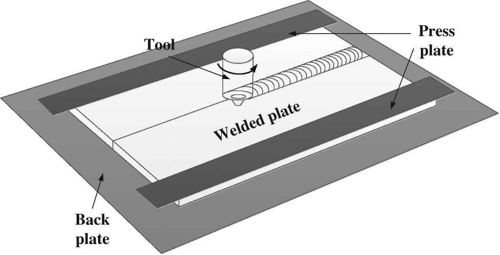
3D solid model of FSW.

Figure 2:

Mesh generation used in simulation.

Boundary conditions

The frictional heat was generated mainly by shoulder and pin during FSW process. The auto-adapting heat source model for numerical analysis was established by Li et al. [11] and considers that frictional heat mainly depends on yield strength of material and tool rotational velocity. Frictional heat generated between shoulder and welded plates can be written as

where QS is shoulder heat input, R0 is shoulder diameter, r0 is pin diameter, ReL(T) is yield strength and ω is angular speed.

Frictional heat generated by pin can be written as

where QP is pin heat input.

During numerical simulation, heat input by shoulder is supposed to be surface heat flux with 12 mm diameter. Heat input by tool is simplified as a uniform volume heat flux with 6 mm diameter and 1.7 mm length. The heat flux can be attained by eq. (1) and eq. (2) and loaded into ABAQUS software through the subroutine.

The simulation of temperature field belongs to the transient thermal conductivity with complex nonlinear problem. The differential equation is described as follows:

where ρ is density, c is specific heat capacity, λ is the thermal conductivity coefficient, q is heat flux, t is time and T is temperature.

From eq. (1), it can be known that heat input is closely related to yield strength of welded materials. The effects of temperature on thermal properties and yield strength of Ti–6Al–4V titanium alloy are both considered in simulation, as shown in Figure 3. The initial temperature of welded plates was supposed to be room temperature (20 °C). Since the density of material is nearly fixed as temperature changing, the density is set to a constant value of 4,450 kg/m³. The thermal conductivity on various surfaces of the welded plate plays an important role in temperature fields. Figure 4 shows the schematic diagram of thermal conductivity applied on the model between the welded plate and surroundings. During the simulation process, the heat loss produced by press and back plates is considered and the constant value of 100 W/(m² °C) is used to describe contact conductivity. For all exposed surfaces, the uniform thermal radiation coefficient and convection coefficient between welded plates and surroundings are respectively set to 0.75 and 50 W/(m² °C) in this paper.

Figure 3:

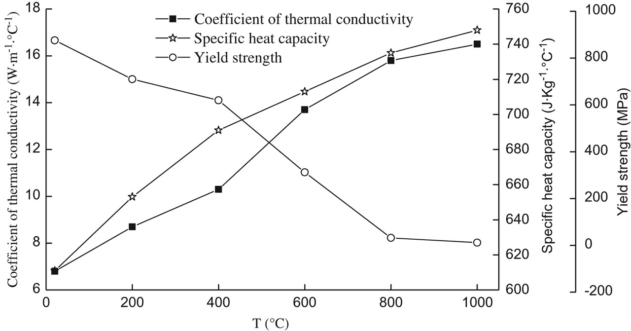
Relation between material parameters used in simulation and temperature.

Figure 4:

Schematic diagram of heat loss used in simulation.

Temperature and experimental verification

Temperature distribution of joint at the rotational velocity of 375 rpm is shown in Figure 5. During FSW process, the material at the rear of the tool experiences frictional heat caused by the direct effect of the tool and subsequent thermal conductivity. The material in front of the tool only experiences thermal conductivity. Therefore, the temperature gradient at the rear of the tool is far less than that in front of the tool (Figure 5). Since the shoulder diameter is bigger than the pin diameter, the area of high temperature near the top surface is wider than that near the bottom surface. Meanwhile, the bottom surface of plate owns relatively higher convection coefficient compared with the top surface. Those two reasons lead to the temperature distribution in the A–A (Figure 5) cross section perpendicular to the weld direction presenting “bowl” shape, as shown in Figure 6.

Figure 5:

Temperature distribution during the FSW process (ω = 375 rpm; ν = 50 mm/min).

Figure 6:

Temperature distribution in the A–A cross section.

In order to verify the validity of temperature field by numerical simulation, NiCr/NiSi thermocouples are used to perform temperature measurement experiment, and the schematic of measuring points is illustrated in Figure 7.

Figure 7:

Schematic of measuring points in the experiment.

The base material (BM) has an initial microstructure characterized by elongated primary α and transformed β, as shown in Figure 8. The white and gray regions in the OM image represent primary α and transformed β phases, respectively.

Figure 8:

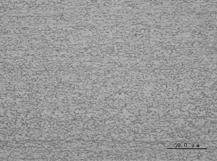
Microstructure of BM of TC4 titanium alloy.

During FSW, the material along the thickness direction experiences diverse thermal cycle due to lower thermal conductivity coefficient of Ti–6Al–4V alloy, which results in different microstructure characteristics. Figure 9 shows the microstructure along the thickness direction at the rotational velocity of 375 rpm. The formation of lamellar microstructure near the joint top surface suggests that the peak temperature is higher than β transus temperature. The results are verified by the temperature distribution of joint in Figure 6. The α + β → β transformation takes place when the peak temperature is higher than β transus temperature at the heating stage. The β → α + β transformation occurs at the cooling stage, resulting in lamellar α + β microstructure due to the relatively high cooling rate. Therefore, the lamellar microstructure is developed in Figure 9(a) and (b). Similar results have also been observed by Ramirez et al. [12] and Mironov et al. [5, 13]. As the distance away from the joint surface becomes longer, peak temperature gradually decreases to a smaller value, which is below β transus temperature (Figure 6). Hence, the microstructure in Figure 9(c) and (d) only consists of primary α and transformed β phases, which was also reported by Pilchak et al. [14, 15] and Zhou et al. [16]. However, compared with BM, the microstructure in Figure 9(c) and (d) is significantly refined because of dynamic recrystallization. Therefore, the microstructure in the present study can verify the rightness of temperature field by simulation.

Figure 9:

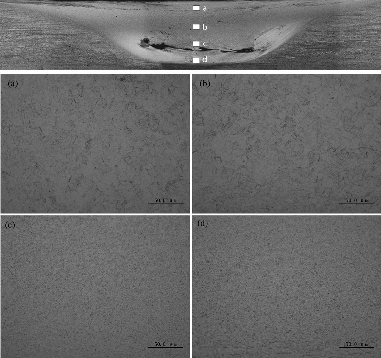
Microstructure of cross section of joints at rotational velocity of 375 rpm: (a) d=0.25 mm, (b) d=0.75 mm, (c) d=1.25 mm, (d) d=1.75 mm (d represents the distance away from weld surface).

Figure 10 shows the comparison of the thermal cycle at the rotational velocity of 300 rpm between simulation and experiment results. It can be seen from Figure 10 that the temperature history curves by simulation are the same as those by experiment. During FSW process, the material in SZ undergoes heating and cooling stage. Temperature of material in SZ rapidly rises at the heating stage while temperature drops quickly at the initial cooling stage and slowly at the later cooling stage. In the experimental process, argon gas synchronously moves along with rotational tool and rapidly cools weld and nearby, which can be considered as strong convection. The region far away from the weld experiences slowly heat loss owing to the weak heat convection. In order to simplify the simulation process, the heat convection coefficient under strong heat convection is applied to the whole weld. Therefore, the difference of temperature between simulation and experiment is relatively large at the later cooling stage (Figure 10). Peak temperatures of points 1 and 2 by experiment are respectively 411.1and 286.2 °C, while the values are 423.8and 288.1 °C by simulation. The deviations of points 1 and 2 are 3.1 % and 0.67 %, respectively. Therefore, the rationality of simulation results can be verified by the experimental results and the temperature field during FSW process can be described perfectly by the FEM established in this study.

Figure 10:

Comparison of thermal cycle between simulation and experimental results.

Temperature history curves of top and bottom surfaces under different rotational velocities are illustrated in Figure 11. It can be seen that the temperature of weld firstly increases and then decreases and the maximum value can be achieved when the rotational tool reaches the researched point. Compared with the bottom surface, the peak temperature of the top surface is higher, which results from the differences of heat flux and heat loss mentioned above. Under the constant welding speed, the peak temperature is mainly decided by the rotational velocity of the tool. Generally speaking, increasing rotational velocity is beneficial to attain higher peak temperature [16, 17]. In this study, when the rotational velocity increases from 120 to 375 rpm, the peak temperature of top and bottom surface increases from 822.1 to 1,091.2 °C, 741.6 to 987.4 °C, respectively.

Figure 11:

Temperature curves of top surface and bottom surface under different rotational velocities: (a) ω = 375 rpm and (b) ω = 120 rpm.

Macrostructure of the joints

Macrographs in cross section of FSW joints under different rotational velocities are shown in Figure 12. It can be observed that the joints are all made up of three distinct zones: SZ, heat affected zone and BM. The SZ exhibits a “bowl” shape significantly widening toward the upper surface, which is mainly related to the temperature distribution (Figure 6). When the rotational velocities vary from 375 to 300 rpm, large tunnel defect appears in SZ. The similar phenomenon was also reported by Mironov et al. [18]. Decreasing rotational velocity is propitious to reduce the size of tunnel defect (Figure 12(c)). The defect-free joint is produced at the rotational velocity of 120 rpm (Figure 12(d)). However, Buffa et al. [9] found that the size of defect at the bottom of Ti–6Al–4V alloy FSW lap joint decreases with the increase of rotational velocity, which is different from the experimental phenomenon in this study. This may result from the different of joint type and tool geometry. So far, there is no detailed analysis about the defect which is just thought to be associated with the relatively low tool rotational velocity. In this study, the tunnel defect is thought to be mainly related to the tensile residual stress of joint. Frictional heat causes the localized expansion of weld. However, the surrounding metal with low temperature restrains the expansion of weld, producing welding compressive stress at the heating stage of FSW. At the cooling stage, the surrounding metal of weld restrains the shrinkage of weld, making tensile residual stress produced. The lower peak temperature during the welding process is beneficial to reduce tensile residual stress. For FSW joint of titanium alloy, the tensile residual stress in SZ appears along the thickness direction because of the different magnitudes of shrinkage caused by temperature gradient between the top surface and the bottom surface. Compared with aluminum alloy, the thermal conductivity coefficient of Ti–6Al–4V titanium alloy is relatively lower, so the obvious temperature difference appears along the thickness direction (Figure 11). Effect of rotational velocities on the temperature difference between the top surface and the bottom surface is shown in Figure 13. It can be concluded that decreasing rotational velocity makes the temperature difference decrease. With the increase of rotational velocities varied from 120 to 375 rpm, the temperature difference increases from 80.5 to 103.8 °C. Soul et al. [19] reported that the rate of welding stress change is proportional to the temperature gradient. The bigger temperature gradient easily produces higher tensile residual stress in weld [20, 21]. Therefore, the joint with lower peak temperature and temperature gradient under lower rotational velocity easily owns lower tensile residual stress. When the tensile residual stress at temperature is higher than the yield stress of Ti–6Al–4V titanium alloy, the material is torn and the tunnel defect may appear (Figure 12(a)–(c)). Meanwhile, the defect-free joint of Ti–6Al–4V titanium alloy is attained under the rotational velocity of 120 rpm due to the lowest peak temperature and smallest temperature gradient in this study (Figure 12(d)).

Figure 12:

Macrostructure of welding joint under different rotational velocities: (a) ω = 375 rpm, (b) ω = 350 rpm, (c) ω = 300 rpm, (d) ω = 120 rpm.

Figure 13:

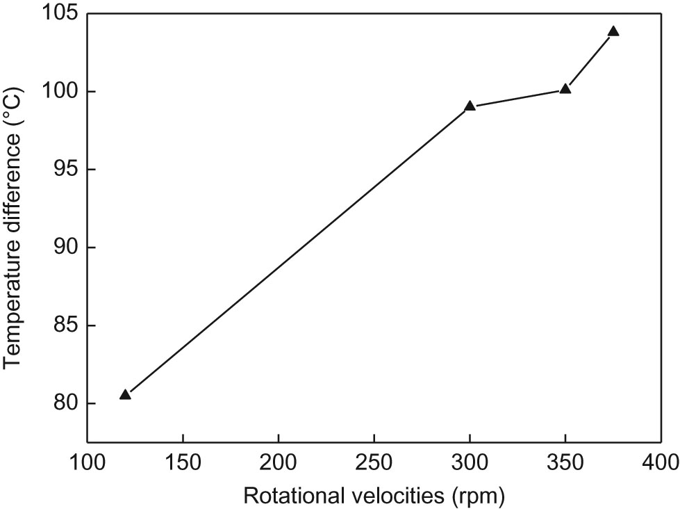
Temperature difference between top surface and bottom surface at different rotational velocities.

References

[1] H.J. Liu, L. Zhou and Q.W. Liu, Mater. Des., 31 (2010) 1650–1655.10.1016/j.matdes.2009.08.025Search in Google Scholar
[2] Z. Shen, Y. Chen, M. Haghshenas and A.P. Gerlich, Eng. Sci. Technol., 18 (2015) 270–277.Search in Google Scholar
[3] L. Zhou, H.J. Liu and L.Z. Wu, Trans. Nonferrous Met. Soc. China, 24 (2014) 368–372. (in Chinese)10.1016/S1003-6326(14)63070-3Search in Google Scholar
[4] Y. Zhang, Y.S. Sato, H. Kokawa, S.H.C. Park and S. Hirano, Mater. Sci. Eng. A, 485 (2008) 448–455.10.1016/j.msea.2007.08.051Search in Google Scholar
[5] S. Mironov, Y. Zhang, Y.S. Sato and H. Kokawa, Scr. Mater., 59 (2008) 27–30.10.1016/j.scriptamat.2008.02.014Search in Google Scholar
[6] H.B. Schmidt and J.H. Hatte, Scr. Mater., 58 (2008) 332–337.10.1016/j.scriptamat.2007.10.008Search in Google Scholar
[7] K.J. Song, Z.B. Dong, K. Fang, X.H. Zhan and Y.H. Wei, Mater. Sci. Technol., 30 (2014) 700–711.10.1179/1743284713Y.0000000389Search in Google Scholar
[8] G. Buffa, J. Hua, R. Shivpuri and L. Fratini, Mater. Sci. Eng. A, 419 (2006) 389–396.10.1016/j.msea.2005.09.040Search in Google Scholar
[9] G. Buffa, L. Fratini, M. Schneider and M. Merklein, J. Mater. Process. Technol., 213 (2013) 2312–2322.10.1016/j.jmatprotec.2013.07.003Search in Google Scholar
[10] M.J. Russell, C. Blignault, N.L. Horrex and C.S. Wiesner, Weld. World, 52 (2008) 12–15.10.1007/BF03266662Search in Google Scholar
[11] H.K. Li, Q.Y. Shi and H.Y. Zhao, Trans. China Weld. Inst., 27 (2006) 81–85. (in Chinese)Search in Google Scholar
[12] A.J. Ramirez and M.C. Juhas, Mater. Sci. Forum, 426 (2003) 2999–3004.10.4028/www.scientific.net/MSF.426-432.2999Search in Google Scholar
[13] S. Mironov, Y. Zhang, Y.S. Sato and H. Kokawa, Scr. Mater., 59 (2008) 511–514.10.1016/j.scriptamat.2008.04.038Search in Google Scholar
[14] A.L. Pilchak, M.C. Juhas and J.C. Williams, Metall. Mater. Trans. A, 38 (2007) 401–408.10.1007/s11661-006-9061-xSearch in Google Scholar
[15] A.L. Pilchak, D.M. Norfleet, M.C. Juhas and J.C. Williams, Metall. Mater. Trans. A., 39 (2008) 1519–1524.10.1007/s11661-007-9236-0Search in Google Scholar
[16] L. Zhou, H.J. Liu and Q.W. Liu, Mater. Des., 31 (2010) 2631–2636.10.1016/j.matdes.2009.12.014Search in Google Scholar
[17] W. Tang, X. Guo and J.C. McClure, J. Mater. Process. Manu. Sci., 7 (1998) 163–172.10.1106/55TF-PF2G-JBH2-1Q2BSearch in Google Scholar
[18] S. Mironov, Y.S. Sato and H. Kokawa, Acta. Mater., 57 (2009) 4519–4528.10.1016/j.actamat.2009.06.020Search in Google Scholar
[19] F. Soul and N. Hamdy, Numerical Simulation of Residual Stress and Strain Behavior After Temperature Modification, Welding Processes, Dr. Radovan Kovacevic (Ed.), ISBN: 978-953-51-0854-2, InTech, DOI: 10.5772/47745 (2012).Search in Google Scholar
[20] Q. Zhao and C. Wu, Eng. Mech., 29 (2010) 262–268. (in Chinese)Search in Google Scholar
[21] B. Niu, X.K. Liu, Z.H. Chen, Z.J. Yang, H.B. Lv and H. Li, J. Build. Struct., 35 (2014) 87–95. (in Chinese)Search in Google Scholar
© 2017 Walter de Gruyter GmbH, Berlin/Boston
This article is distributed under the terms of the Creative Commons Attribution Non-Commercial License, which permits unrestricted non-commercial use, distribution, and reproduction in any medium, provided the original work is properly cited.
Articles in the same Issue
- Frontmatter
- Research Articles
- Experimental Study on Application of Boron Mud Secondary Resource to Oxidized Pellets Production
- A Study at the Workability of Ultra-High Strength Steel Sheet by Processing Maps on the Basis of DMM
- Oxidation Behavior of TiAl-Based Alloy Modified by Double-Glow Plasma Surface Alloying with Cr–Mo
- Transient Liquid Phase Bonding of Nickel-Base Single Crystal Alloy with a Novel Ni-Cr-Co-Mo-W-Ta-Re-B Amorphous Interlayer
- Effects of Mn and Al on the Intragranular Acicular Ferrite Formation in Rare Earth Treated C–Mn Steel
- Effect of Plate Thickness on Tensile Property of Ti–6Al–4V Alloy Joint Friction Stir Welded Below β-Transus Temperature
- Characterization of High Temperature Deformation Behavior of BFe10-1-2 Cupronickel Alloy Using Orthogonal Analysis
- Influence of Ni Additions on the Viscosity of Liquid Al2Cu
- Corrosion Process of Stainless Steel 441 with Heated Steam at 1,000 °C
- Influence of Ti on the Hot Ductility of High-manganese Austenitic Steels