A Computer Program for Practical Semivariogram Modeling and Ordinary Kriging: A Case Study of Porosity Distribution in an Oil Field

Bayram Ali Mert; Ahmet Dag

doi:10.1515/geo-2017-0050

Article Open Access

A Computer Program for Practical Semivariogram Modeling and Ordinary Kriging: A Case Study of Porosity Distribution in an Oil Field

Bayram Ali Mert and Ahmet Dag

Published/Copyright: December 29, 2017

Published by

Become an author with De Gruyter Brill

Submit Manuscript Author Information

From the journal Open Geosciences Volume 9 Issue 1

Abstract

In this study, firstly, a practical and educational geostatistical program (JeoStat) was developed, and then example analysis of porosity parameter distribution, using oilfield data, was presented.

With this program, two or three-dimensional variogram analysis can be performed by using normal, log-normal or indicator transformed data. In these analyses, JeoStat offers seven commonly used theoretical variogram models (Spherical, Gaussian, Exponential, Linear, Generalized Linear, Hole Effect and Paddington Mix) to the users. These theoretical models can be easily and quickly fitted to experimental models using a mouse. JeoStat uses ordinary kriging interpolation technique for computation of point or block estimate, and also uses cross-validation test techniques for validation of the fitted theoretical model. All the results obtained by the analysis as well as all the graphics such as histogram, variogram and kriging estimation maps can be saved to the hard drive, including digitised graphics and maps. As such, the numerical values of any point in the map can be monitored using a mouse and text boxes. This program is available to students, researchers, consultants and corporations of any size free of charge. The JeoStat software package and source codes available at: http://www.jeostat.com/JeoStat_2017.0.rar

Keywords: Variogram; Kriging; Geostatistics; Spatial Analyses; Visual Basic; Reservoir

1 Introduction

Geostatistics include a number of methods and techniques to analyze the variability of spatially distributed or spatially structured regionalized variables [1]. The techniques, developed by Krige [2] and Matheron [3] to evaluate orebody, have been disseminated out into many other fields, utilising spatial data. Its diverse disciplines include petroleum geology [4], hydrogeology [5], hydrology [6], meteorology [7], oceanography [8], geochemistry [9], metallurgy [10], geography [11,12], forestry [13], environmental control [14], landscape ecology [15], soil science and agriculture [16, 17]. In petroleum industries, geostatistics is successfully applied to characterize petroleum reservoirs based on interpretations from sparse data located in space, such as reservoir thickness, porosity, permeability and seismic data [18,19,20]. The basic steps of a geostatistical analysis consist of creating an experimental semivariogram, fitting a model to the experimental semivariogram and using the information from this to carry out the kriging. Analyzing the spatial continuity or roughness of a geospatial data in different directions and tolerances, called semivariogram analysis, is time-consuming. Furthermore, performing the cross-validation to the semivariogram model and inputting test parameters of every model in various directions and tolerance angles requires a computer program, since it is almost impossible to manually perform these analyses which require a large number of numerical calculations. Many computer programs have been developed including Geo-EAS [21], GSLIB [22], Variowin [23], GSTAT [24], S-GeMS [25], etc . When the most of the commercially available programs assessed, it was notified that some of those programs are not providing an opportunity to fit some of the model semivariograms and/or to present outputs of some stages of the analysis and also especially semivariogram analysis for different directions or anisotropy might take a lot of time. Some software which is public domain such as Geo-EAS [21], runs under MS-DOS platform. Those ones are not up-to-date for running on Windows platforms. Although they are useful in research and education, their potential application is limited as they are not suitable for Windows. Besides, most programs (e. g., Geo-EAS [21], GSLIB [22], Variowin [23]) do not allow to analyze 3D data and contain the very limited number of theoretical semivariogram models. In this context, Geo-EAS [21] contains only four different theoretical semivariogram models. Furthermore, indicator- and log-kriging is occasionally needed in the spatial data analysis; most of the freely available programs have no tools to do such analysis. More importantly, just a few of programs allow the user to estimate values for a convex or concave polygon area, although required in reserve estimation in the mining sector. All those shortcomings constrain analysis of spatial dependence structure of data and may present challenges in teaching as well. In this context, a program is necessary to provide useful outputs to the practitioners as well as instructors who are engaged in the numerical calculations.

The objectives of this study were twofold: a) To develop a user-friendly public domain software for performing geostatistical analysis in geosciences, b) To apply the software to an oil field discipline for modelling porosity and its spatial distribution.

2 Basics of Geostatistical Estimations

In any geostatistical analysis, there are two major steps: a) Semivariogram analysis, b) Kriging estimation and mapping. More generally, that can be divided into four steps to complete fully geostatistical analysis and mapping of regionalized variables [26,27,28]:

i. Determining an appropriate theoretical semivariogram models, used to fit experimental semivariogram and possible anisotropy, ii. Performing validation methods to the semivariogram model,

iii. Generating kriging estimates and errors of estimates, i.e. kriging errors, for a point, zone or volume by kriging interpolation techniques,

iv. Mapping the spatial distributions of the kriging estimates and kriging errors (Fig. 1).

Figure 1

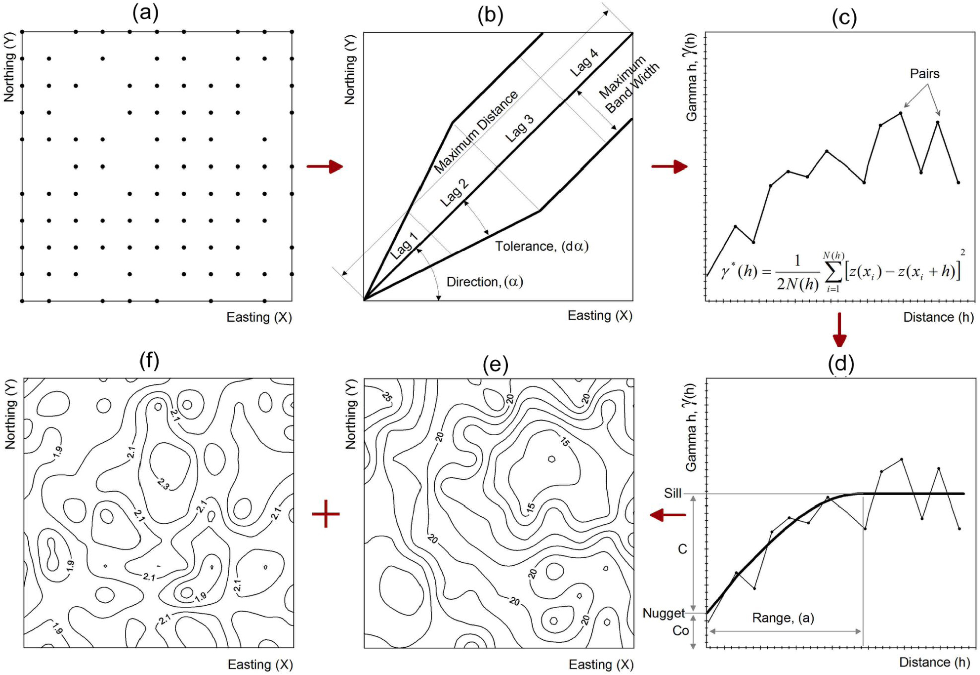
Geostatistical analysis stages: a) post plot of sample data, b) tolerance angles and distance tolerances, c) experimental semivariogram, d) theoretical semivariogram, e) contouring of kriged values, f) kriging error map

In a geostatistical analysis, all these components must be systematically accounted for [29,30,31].

2.1 Semivariogram Analyses

The semivariogram is a plot of semivariances as a function of distances between the observations, and is denoted by γ(h) [32,33,34]. In order to plot experimental semivariogram, firstly, N(N-1)/2 pairs of combinations are formed from the N observations [22, 26], and Euclidean distances (h) and direction angle (α) between pairs are calculated by the following equations [27].

h=ui−uj=(xi−xj)2+(yi−yj)2+(zi−zj)2;ui=(xi,yi,zi),uj=(xj,yj,zj)(1)

α=arctangent yi−yjxi−xj(2)

where u_iand u_j are observation locations; x_i, y_i, z_i are easting, northing and elevation, respectively.

Secondly, observation pairs are classified in different direction angles, distance conditions and the semivariance between them is calculated with the help of Eq. (3). Finally, the semivariance values calculated for each distance (h) are plotted and an experimental semivariogram is obtained [35] as shown in Fig. 2a.

γ∗(h)=12N(h)∑i=1N(h)[z(xi)−z(xi+h)]2(3)

Figure 2

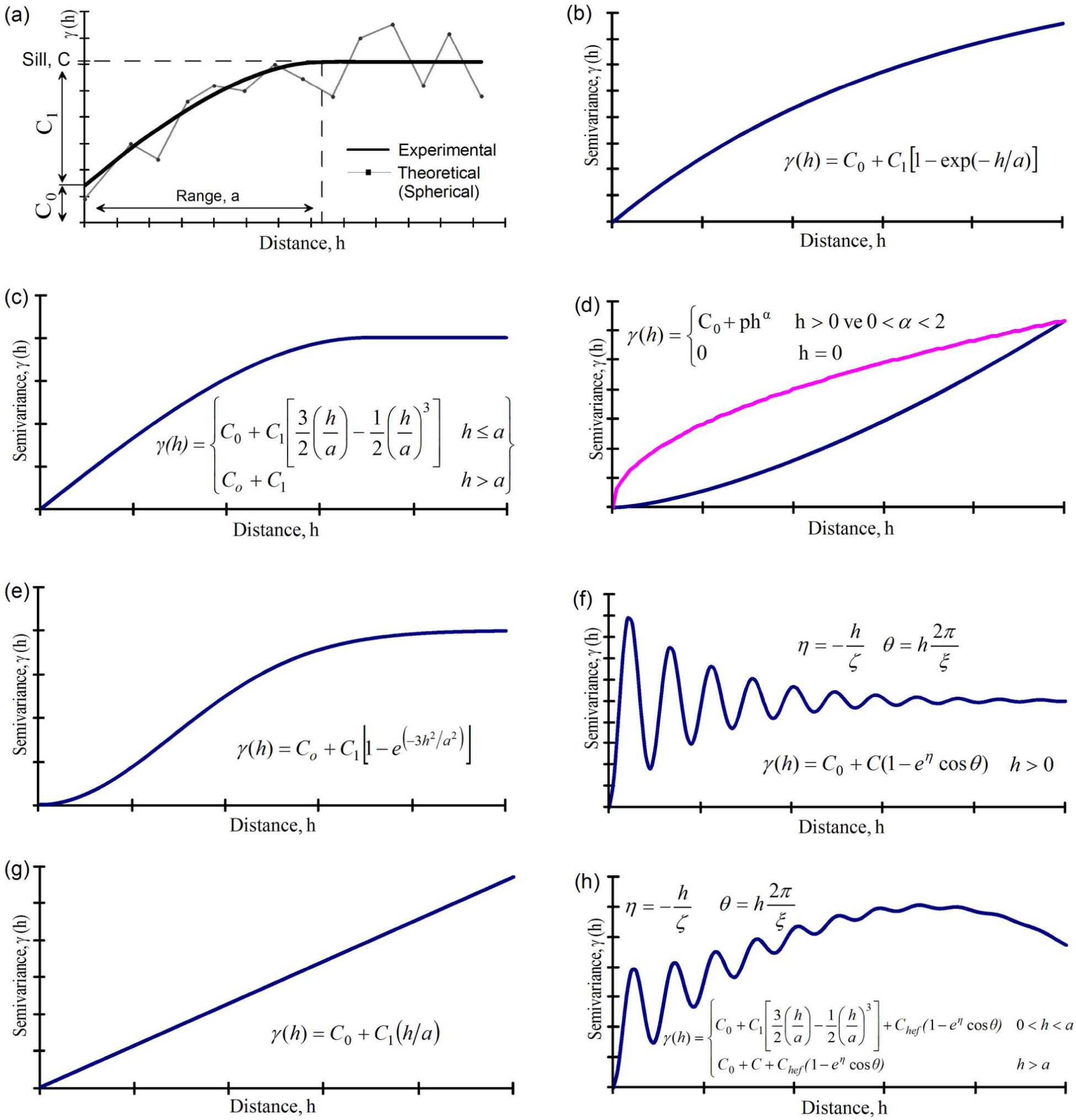
Example of experimental and theoretical semivariogram model; commonly used theoretical semivariogram models: (b) Exponential, (c) Spherical, (d) Generalized linear, (e) Gaussian model, (f) Hole effect, (g) Linear (h) Paddington mix.

where zis an observed value at a particular location, his the distance between ordered data, and N(h) is the number of paired data at a distance of h [31].

Before using experimental semivariogram in the kriging estimation process, the most appropriate theoretical model representing the experimental semivariogram needs to be determined. Commonly used theoretical models are presented in Fig. 2(b-h) [21, 26]. C₀; C₁ and C are the nugget (unaccountable) and stochastic (accountable) variance; sill value [17], respectively; and a is the range of influence [23].

In JeoStat, data is assumed to be stationary, i.e. there is no trend in the data. If that data is not stationary, trend needs to be removed using following trend surface analysis [36]. Subsequently, detrended data can be easily analysed by JeoStat program.

2.2 Cross-Validation

One of the commonly used methods to verify the validity of the selected semivariogram models and their parameters is ‘jack-knifing’ cross-validation [37, 38]. The technique compares estimated and observed values at the geographical locations. The sample value at a particular location is discarded intentionally from the sample data set, and the value at the same location is estimated using the remaining dataset, adopted semivariogram and estimated parameters [39]. The process, therefore, provides an observed and estimated value for each data location (i). The estimated value can then be compared to the observed value. To this end, reduced variable (RE), mean reduced error (MRE) and reduced variance (RVAR) are calculated using the equations [17, 40]

REi=Zi∗−ZiσOKiMRE=1N∑i=1NREiRVAR=1N−1∑1N(REi−MRE)2(4)

where Z^*_i, Z_i, σ_{OK_i} are estimated and observed values, kriging standard deviation or kriging error, respectively. Jeo-Stat program employs ‘jack-knifing’ cross-validation technique for validating postulated theoretical semivariogram and adopted parameters.

2.3 Ordinary Kriging Interpolation

The adopted theoretical semivariogram and its parameters can be used interactively in the Jeostat program to estimate unknown values at unsampled locations as well as to quantify various features of the regionalized variable. Kriging, which serves this purpose, is used as a best linear unbiased estimator (BLUE) [14, 41, 42]. Simple, ordinary and block interpolation are the most common estimation techniques. However as the true value of the population is usually unknown ordinary and block kriging techniques [17, 35, 36] are adopted in this study to ensure an unbiased estimated value. If the kriging estimator is used to estimate a value at a particular location u_o or an average value in an area (block) or volume (V) centred at u_o, the estimate (Z^*_V) for a continuous variable [4] can be given in a general form:

Z∗V=1V∫VZ(u)dx(5)

Since this estimate of Z^*(u₀) gives the value at a location of uo for the numerical function of Z(u), the estimation given in Eq. (5) can be expressed in a discrete form as the linear sum of the observed values with the Eq. (6) [43].

Z∗V(u0)=∑i=1nλiZ(ui)(6)

where Z_v^*, Z(u_i), λ_i are estimated value at u₀, a value of the observations to be used in the estimation of point u₀, sample weighting factor. In order to get an unbiased estimate with the minimum variance [44], Lagrangian Multiplier method [45] is applied and kriging equation set is obtained as in Eq. (6).

∑j=1nλjγui,uj+μ=γ(ui,u0)i=1,2,3,....,n∑i=1nλi=1(7)

σ2OK=∑i=1nλiγ(ui,u0)−γ(u0,u0)+μ(8)

where γ (u_i, u_j), γ(u_i, u₀), stand for semivariance between u_i and U_j observation locations, observation location u_iand the location to be estimated (u_o); μ Lagrangian Multiplier. Following [46], the kriging system of Eq. (7) will take the following matrix form:

A=γ1,1γ1,2γ1,3………………γ1,n1γ2,1γ2,2γ2,3………………γ2,n1γ3,1γ3,2γ3,3………………γ3,n1⋮⋮⋮⋮⋮⋮⋮1⋮⋮⋮⋮⋮⋮⋮1⋮⋮⋮⋮⋮⋮⋮1γn,1γn,2γn,3………………γn,n111111110B=λ1λ2λ3⋮⋮⋮λnμC=γ(u1,u0)γ(u2,u0)γ(u3,u0)⋮⋮⋮γ(un,u0)1(9)

The weights λ_i can be obtained by taking the inverse of the matrix A and multiplying it by the C vector (Eq. 10). λ_i and μ are found by matrix multiplication as shown in Eq. (11).

B=A−1xC(10)

The variance of the estimate can be calculated by employing Eq. (11).

σ2OK=BTC−γ(uo,u0)(11)

where B^T stands for transpose of vector B. Equations from 6 to 11 are used for point kriging estimation. If block kriging is applied, semivariance terms of γ(u_i, u₀) and γ(u₀, u₀) should be substituted for γ(u_i, V) and γ(V, V), respectively, in order to ensure areal or volume estimates.

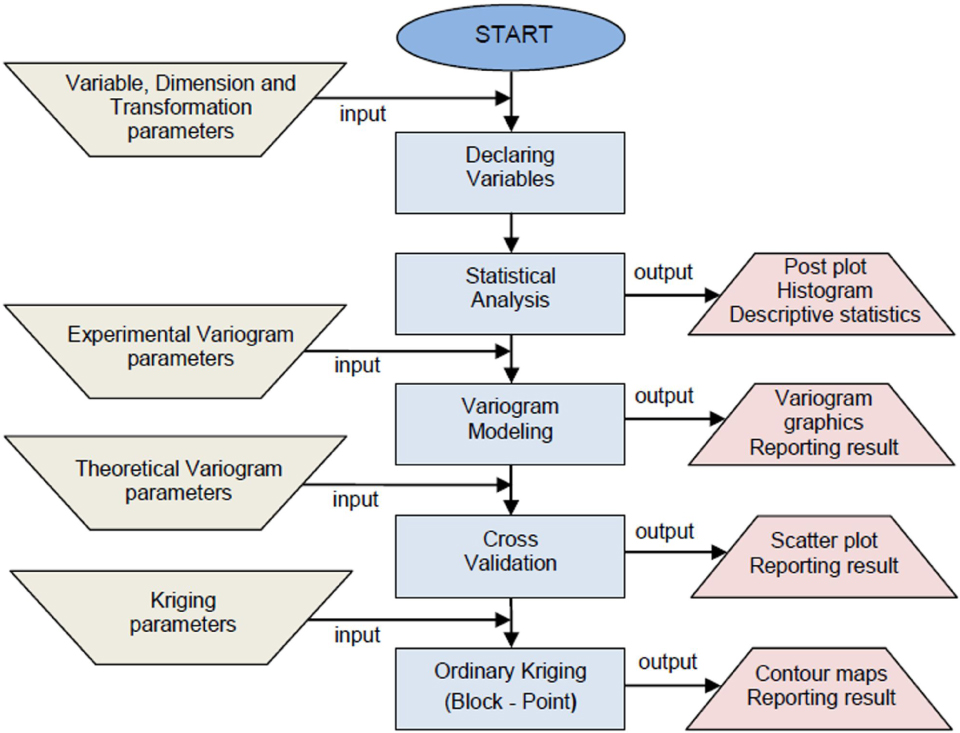
3 Details of JeoStat

Semivariogram analysis techniques and kriging estimation equations are implemented in the JeoStat software using Visual Basic language. JeoStat main application form includes six tab screens. These tabs are, in order;

Importing data,
Statistical analysis,
Semivariogram modeling,
Cross-validation test,
Kriging estimates and variances,
Visualization of the outputs.

JeoStat’s general flowchart is shown in Fig. 3, and analysis details are described in the following sections.

Figure 3

General flowchart for JeoStat

3.1 Preparing and Importing Data

The JeoStat file format is aimed to be as simple as possible. The data file is an ASCI file with headers lines followed by the data, which is tab or comma delimited. As shown in Fig. 4, the first header line is a title. The second line should be a numerical value specifying the number of numerical variables in the data file. The next lines contain character identification labels. The following lines are considered as data points and must have numerical values per line. Declaring variable sized array in JeoStat is programmed by using a method called “Dynamic Array Allocation”, which allows the program to analyze any size data set, up to limit of a user’s machine memory.

Figure 4

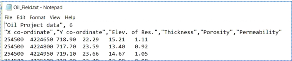
Data file in ASCII format

Once the data file has been prepared, it can be loaded by clicking the “Input File” button. On the second stage, a user should select and define variables required for the statistical analysis which are UTM coordinate columns (X (easting), Y (northing) and elevation), variable label and dimension of analysis, as well as transformation options from the combo box components. Once the variables have been declared, preliminary information such as a number of pairs, maximum and minimum values on tab screen is obtained by clicking “Read Data”. If the user will perform an analysis based on an indicator or logarithmic transformation [26, 30, 41], the values of cut-off or log option must be entered in required text boxes (Fig. 5). When the user selects “Three Dimensional” option from Combo Box, parameters regarding three-dimensional analyses will be activated automatically on the other tabs’ screen. Additionally, there is a text box under the file menu of the screen where the user can enter the path and name of the output file, which will be saved to the hard drive with various file extensions such as “stat” for statistical analysis results, “var” for semivariogram analysis results, 11res” for cross validation results and “grd” for kriging results file.

Figure 5

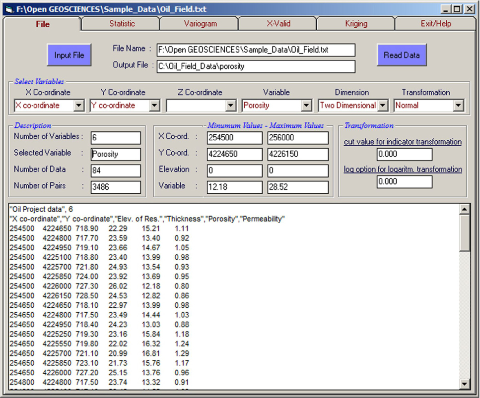
A captured view of the JeoStat’ data importing window

3.2 Statistical Analysis

Descriptive statistics are used to describe the basic features of the data in a geostatistical study. To this end, Jeo-Stat offers various descriptive statistics [47] such as variance, standard deviation, median, mean, skewness, kurtosis, coefficient of variation, minimum and maximum values (Fig. 6). Additionally, histogram and post plots of the spatial data can be displayed easily on the screen (Fig. 7). Visual Basic Picture Box objects displaying graphics were digitized during the program development process so the user easily observe the abscissa and ordinate values of the graphics by moving mouse, also all the graphics can be saved to the hard drive.

Figure 6

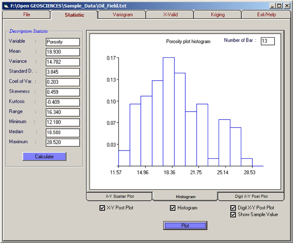
“Statistics tab screen” of JeoStat for delineating histogram and descriptive statistics of porosity data

Figure 7

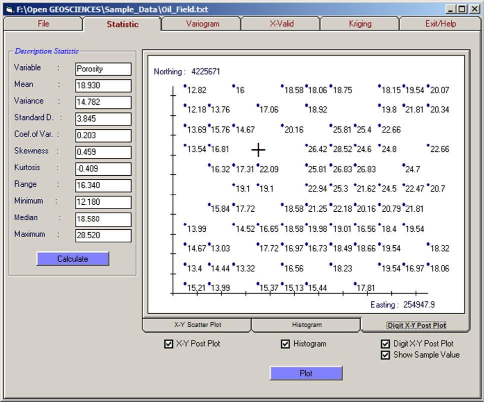
JeoStat “Statistics tab screen” for post plot of observed porosity data

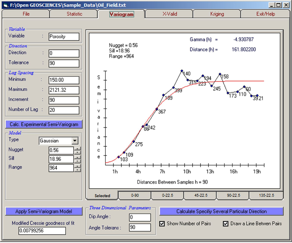
3.3 Semivariogram Analysis

The tab of the window frame contains text boxes for parameters required modelling the experimental semivariogram, such as direction, tolerance angles, number of lag and lag distance. After the parameters have been entered and “Calculate experimental semivariogram” button clicked, the experimental semivariogram graphic for the selected parameters can be monitored in the picture box labelled “selected”. This means that the user can select whatever direction and tolerance angle he wants. In addition, there are also predefined direction and tolerance angles such as 0°-22.5°. By clicking “Calculate specify particular direction” button, experimental semivariogram graphics for the predefined direction and tolerance angles of 0°-90°, 0°-22.5°, 45°-22.5°, 90°-22.5° and 135°-22.5° can be easily monitored on the other picture boxes, for anisotropy or for computation of experimental semivariograms for different directions (Fig. 8). The obtained experimental semivariogram graphics can be customized by activating “show number of pairs” and “draw a line between pairs” checkboxes.

Figure 8

A view of the JeoStat’ semivariogram analysis screen

It is important to highlight that JeoStat includes the commonly used theoretical semivariograms models given in Fig. 2. These are spherical, gaussian, exponential, linear, generalized linear, hole effect and paddington mix. Once a set of experimental semivariogram is computed, one of the theoretical semivariogram models is chosen from a combo box. Subsequently, the model’s parameters can be modified either by mouse events on the graphics or by entering a plausible value to the textboxes by hand or clicking the scroll bar for easily and quickly fitting. Alternatively, theoretical model parameters can be entered by clicking a mouse on the semivariogram screen. The program employs two types of testing techniques for validating the model semivariogram. One of the testing methods is “Cressie goodness-of-fit” model [34], in which testing result is presented to the user in a text box on this tab screen for the prior knowledge of the user. The other testing method, cross validation, can be performed on the other tab screen of the JeoStat.

The numerical results of the experimental and theoretical semivariogram models computed in this tab are saved on a file with “var” extension and, if desired, the user can use these results to draw semivariogram graphics on another program, such as Microsoft Excel. All the graphics from this screen might be saved to hard drive as an image file “jpg”.

3.4 Cross Validation Test

This program utilizes Eq. (4) to validate theoretical semivariogram model. For this purpose, JeoStat automatically imports necessary semivariogram parameters – determined preliminarily by using “Cressie goodness-of-fit” in section 3.3-from the previous tab screen without needing to enter manually into the text boxes. However, if users need to, these parameters can be entered manually as well. During the test, after entering the model and search ellipse parameters into the relevant text boxes and clicking “Cross Validation” button, the user can be monitored the test results and graphics on the screen (Fig. 9).

Figure 9

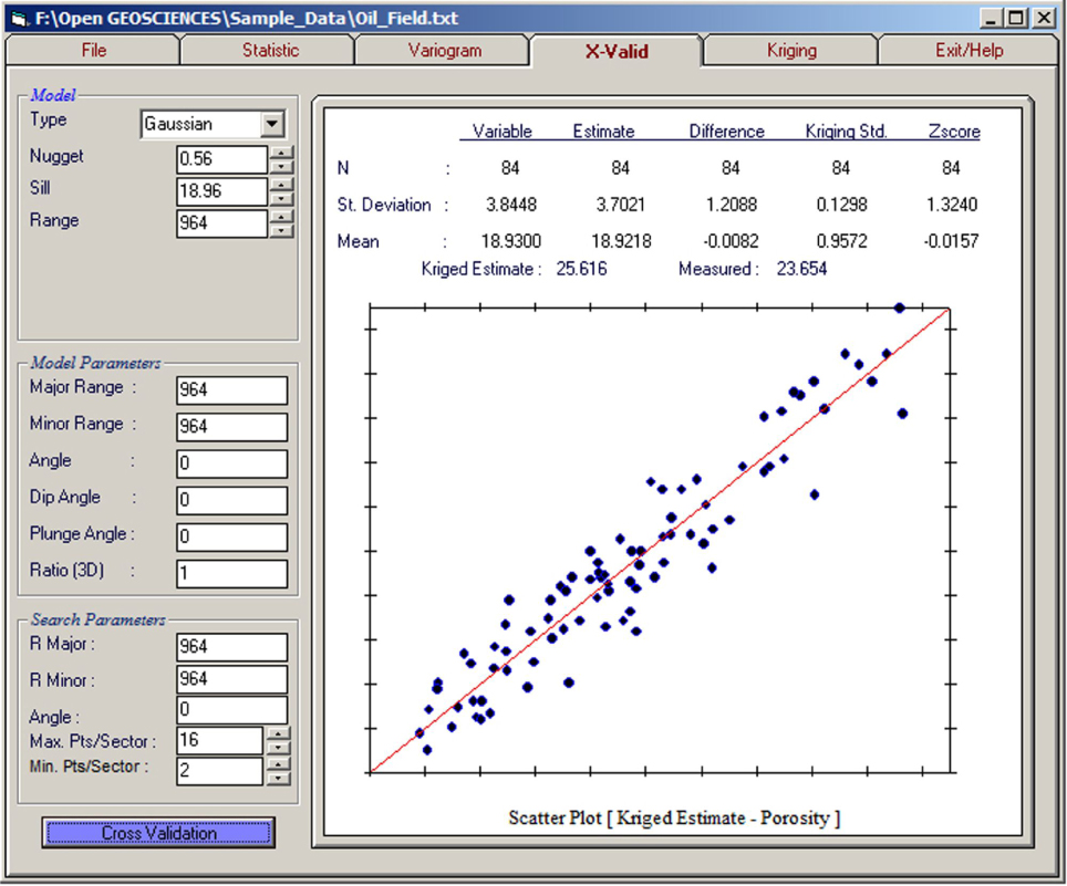
A view of the cross validation test

The numerical results of the cross-validation are saved on a file with “res” extension. For example, the numerical results were automatically saved as “Porosity.res” in this study, The user can use these results to draw a scatter plot on another program. All the graphics from this screen can be saved to hard drive by mouse click events.

3.5 Kriging Interpolation

Point or block estimations can be computed on this tab screen by using Ordinary Kriging interpolation technique given in Eqs. (6-11). For this, firstly, the grids are defined for the region that the estimation will be performed on and then these grids estimates are performed using theoretical semivariogram functions determined on the previous screen.

At this stage of the JeoStat, the user defines the grid dimensions by entering the number of grids and grid distance on the text boxes to divide the prediction region into two or three-dimensional grids. The number of grids and grid size are user dependent. JeoStat allows the user to perform estimation for the whole rectangular region or only for the specified irregular or regular polygonal region. If the user performs the Ordinary Kriging estimations on grids located in a certain polygon, firstly the checkbox must be checked to load convex or concave polygon dataset (Fig. 10). After the grid has been defined, the user can enter the parameters for the search ellipse or required kriging from the screen as seen in Fig. 11.

Figure 10

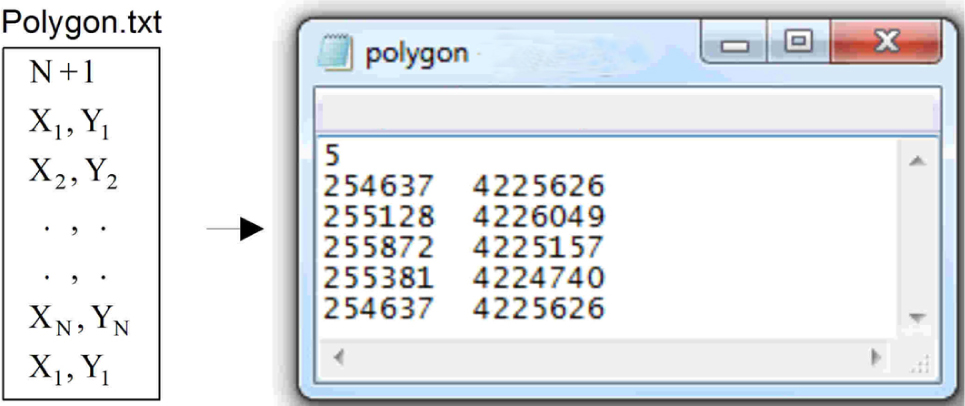
Polygon dataset format

Figure 11

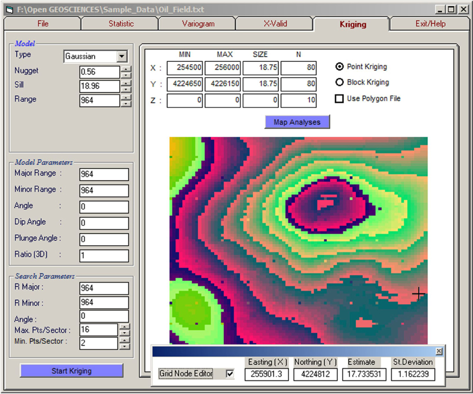
Demonstration of estimate and kriging variance using mouse events applied to mapped kriging results

The numerical results of kriging estimations and estimation errors (kriging standard deviation) in this tab screen are saved with a “grd” extension file and, if needed, the results can be plotted with another program. Additionally, “Grid Node Editor” helps the user to see kriged estimates or kriging errors values through moving the mouse (Fig. 11).

3.6 Visualization of the Outputs

A Contouring Subroutine (Conrec) developed by Bourke [48] and JCBLOK developed by Carr and Mela [49] were integrated into JeoStat to enable contouring and visualization of estimation results. To do contouring of kriging estimates (Eq. 6) and estimation errors (kriging standard deviation) (Eq. 8) in JeoStat, a user only need to enter the data surface and the contour levels want to draw. The contour maps are presented to the user as fully digitized in JeoStat. As such, by using a mouse, the numerical values (easting, nothing, kriging estimates and estimation errors) of any point value in the map can be viewed on the text boxes (Fig. 11).

4 Case Study

In this case study, we applied the geostatistical modelling to analyze an example oil field porosity data, available as a JeoStat’s sample data file. In order to identify variance structure of porosity measurements, experimental semivariance values in different directions and distances were calculated using Eqs. (1-3) and JeoStat. Resulting semivariograms were plotted (Fig. 8, Fig. 12). The experimental semivariogram exhibited a parabolic behaviour around the origin and reached its sill value asymptotically, indicating that a Gaussian model (Fig. 1e) would show a good fit (Fig 12a). Data set was used in GeoEAS [21] and Variowin [23] to check Jeostat program results of experimental semivariograms. It was observed that JeoStat semivariances are exactly the same with those ones, indicating that mathematical algorithms in JeoStat are correct.

Figure 12

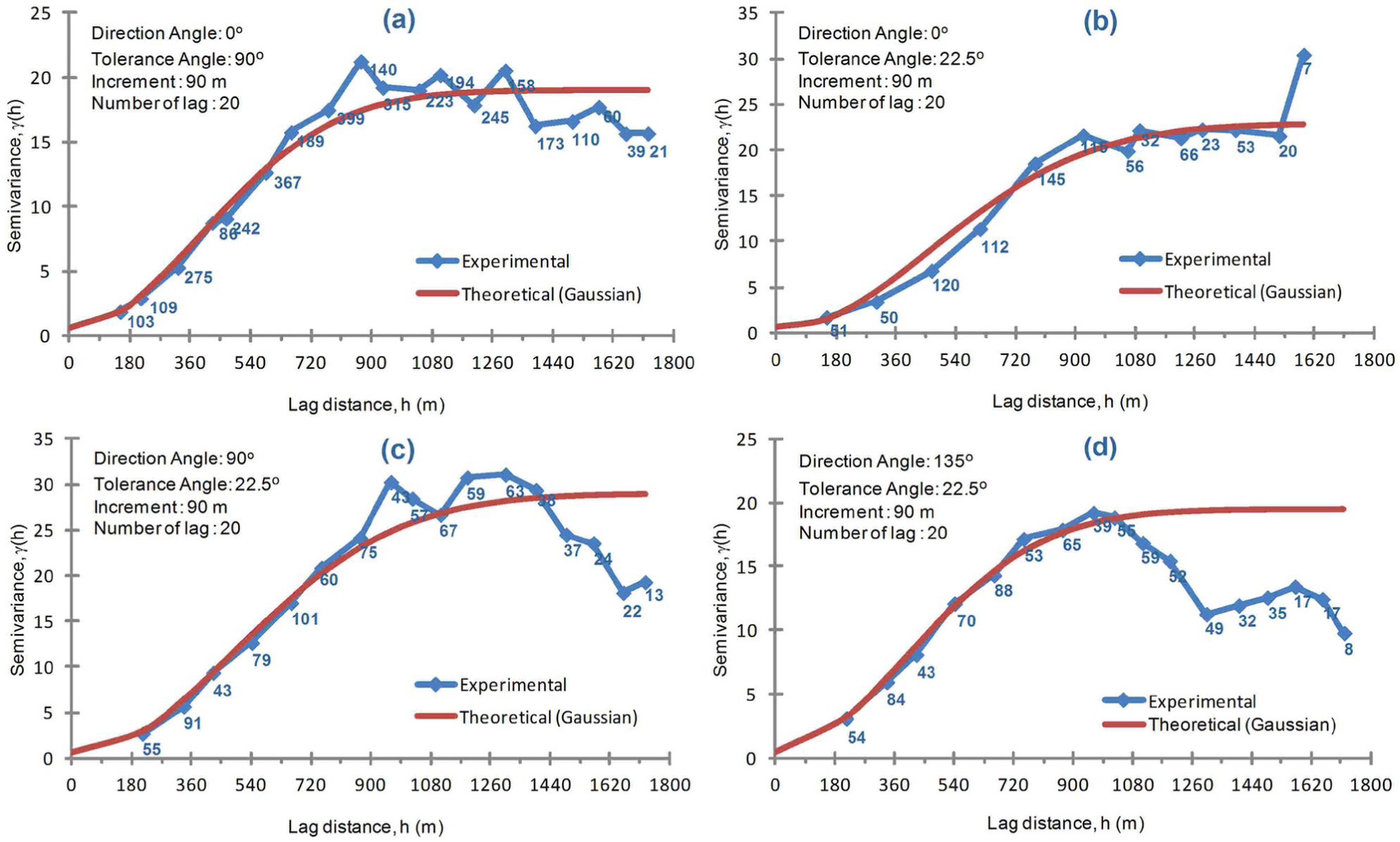
Experimental (line with markers) and theoretical semivariogram (continuous line) models for porosity data set

Jack-knifing cross-validation procedure was carried out to check if theoretical semivariogram models were well fitted to the data. Fig. 7 summarizes cross-validation results. In this method, the data were one by one removed from the 96 actual values and estimated from the remaining 95 data by means of the Ordinary Kriging technique. In the estimations, at most 16 and at least 2 observation values falling under the kriging search dimension were used. MRE and RVAR were calculated based on Eq. (4). In order to carry out an impartial estimation according to Clark and Harper [25], the variance of the reduced errors (RVAR) is expected to be “1” or within 1 ± 22/N (N being number of data points), and their average (MRE) is expected to be “0”. In the current analysis the average of the reduced error, −0.0157 is as close as 0.00 and their variance is within 1 ± 22/95.. As a result, it is possible to state that the selected semivariogram model parameters were valid and expectable for estimation of the porosity at the unsampled locations (Fig. 9). It is important to state that cross-validation results of GeoEAS [21] were rather congruent with the results of JeoStat program.

With the definition of the correlation functions depending on the distances of the variable of porosity value, it is now possible to estimate how these variables are distributed along the reservoir. For this purpose, at first oil field boundaries (Polygonal area in Fig. 10 and Fig. 13) were defined as a polygon area with known coordinates, as presented in Fig. 13. Then, the study area with the UTM coordinates of 254500 − 256000 (east-west), 4224650 − 4226150 (north-south) was divided into a total of 6400 blocks with the dimensions 18.75 m × 18.75 m. The average porosity value of each block was estimated via the ordinary block kriging method (Eq. 7, Fig. 11) to get table data. Porosity contour map (Fig. 13) was generated by using table data.

Figure 13

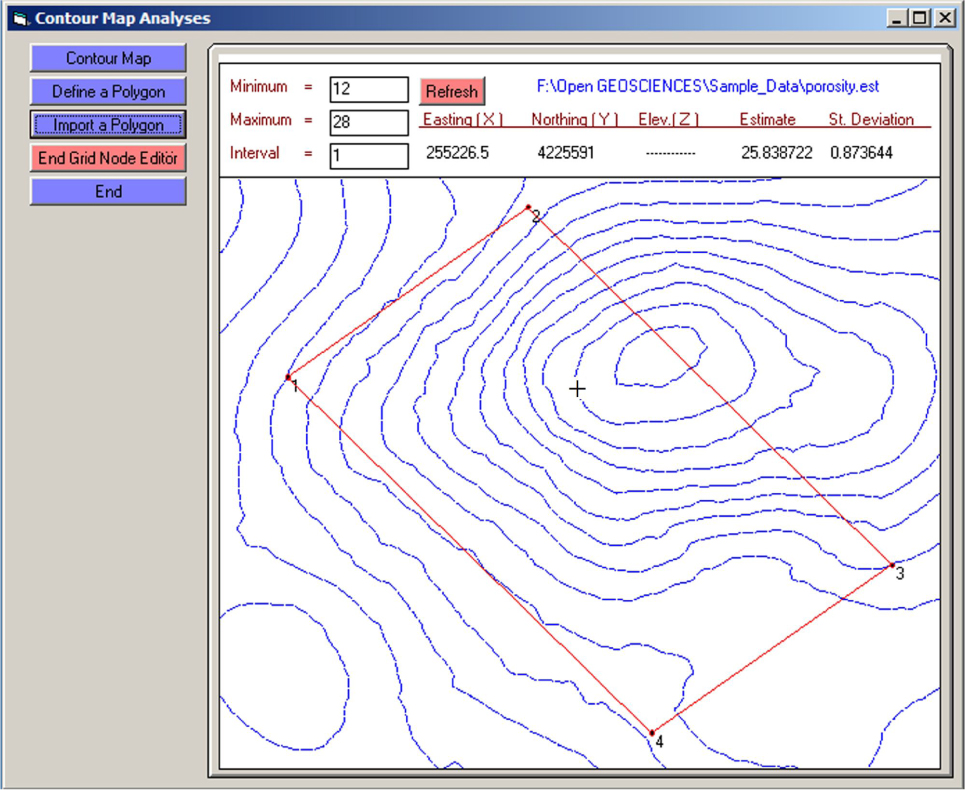
A view of “Grid Node Editor” for porosity contour map of the kriging estimation. Polygonal area stands for oil field boundaries

The user can get estimated values at any grid-cell by moving a mouse on the screen. Thus, kriged estimates and kriging errors of the cell, as well as coordinates, are shown on the label. For example, as seen in Fig. 13, the cursor was located on the u(255226.5, 4225591) coordinate; at this point, kriged porosity is 25.83 and kriging error is 0.87. It must be highlighted that of JeoStat is not a contouring program. Therefore, it was not aimed at assigning values to the contour lines in Figure 13. Contrary to this, JeoStat provides an advantage to the user for visual inspection of the map by using “Grid Node Editor”. This trait of the program is important for detecting errors in the data or getting estimated values for grids. Furthermore, kriging error values lead us to make a decision on the efficiency of sampling used in mapping.

The user of JeoStat can also export kriged estimates, located in the polygonal area presented in Figure 13, as ^*.txt file. This file may be used in complex contouring programs such as Golden Software [50] or any GIS software to generate cartographic maps. Then, elegant maps as shown in Figure 14 might be produced in other platforms without carrying out further geostatistical analysis.

Figure 14

A view of A porosity map generated by Surfer 8.01 [50] using JeoStat results

5 Conclusions

In this study, a program, namely, JeoStat for the spatial analysis has been developed by using a Visual Basic program. Capabilities of the JeoStat program have been described trough utilizing the sample data set of the porosity. The program is able to compute through all the main steps of the basic geostatistical analysis, including semivariogram modelling, cross-validation and ordinary block kriging. Furthermore, the same data set was used in another commercial and public domain programs to compare the validity of JeoStat results. Comparisons of JeoStat program outputs with the outputs of other programs lead us to conclude that JeoStat was able to produce dependable results. Because of its true and dependable outputs plus easy accessibility via the internet, JeoStat is readily available to students, researchers, consultants and corporations of any size. As such, this program has been used by the authors in teaching activities for 3 years and it has been observed that the students can easily understand the courses’ theoretical background when they play with their own data by using such freely available software. It also helps students to comprehend how spatial data might be evaluated with the aid of a computer. Students also attain concept of computer-aided valuation and learn commercial software easily in further advanced courses.

Acknowledgement

The authors would like to thank Dr. Mahmut Cetin (Cukurova University, Department of Irrigation Engineering) for reading the manuscript, making some corrections and his valuable suggestions.

A Appendix

JeoStat software package, source codes and sample data files are available at http://www.jeostat.com/JeoStat_2017.0.rar

References

[1] Hatvani, I. G., & Horváth, J., A Special Issue: Geomathematics in practice: Case studies from earth- and environmental sciences–Proceedings of the Croatian-Hungarian Geomathematical Congress, Hungary 2015. Open Geosciences, 2016, 8(1), 1-4.10.1515/geo-2016-0001Search in Google Scholar

[2] Krige, D. G., A statistical approach to some basic mine valuation problems on the Witwatersrand. Journal of the Southern African Institute of Mining and Metallurgy, 1951, 52(6), 119-139.Search in Google Scholar

[3] Matheron, G., Principles of geostatistics. Economic geology, 1963, 58(8), 1246-1266.10.2113/gsecongeo.58.8.1246Search in Google Scholar

[4] Hohn, M.E., Geostatistics and Petroleum Geology, 2ed. Springer Science+Business Media Dordrecht, The Netherlands, 199910.1007/978-94-011-4425-4Search in Google Scholar

[5] Hatvani, I. G., Magyar, N., Zessner, M., Kovács, J., & Blaschke, A. P., The Water Framework Directive: Can more information be extracted from groundwater data? A case study of Seewinkel, Burgenland, eastern Austria. Hydrogeology Journal, 2014, 22(4), 779-794.10.1007/s10040-013-1093-xSearch in Google Scholar

[6] Kovács, J., Korponai, J., Kovács, I. S., & Hatvani, I. G., Introducing sampling frequency estimation using variograms in water research with the example of nutrient loads in the Kis-Balaton Water Protection System (W Hungary). Ecological engineering, 2012, 42, 237-243.10.1016/j.ecoleng.2012.02.004Search in Google Scholar

[7] Kohán, B., Tyler, J., Jones, M., & Kern, Z. (2017). Variogram analysis of stable oxygen isotope composition of daily precipitation over the British Isles. In: EGU General Assembly Conference Abstracts, Vienna, Austria, 2017, 19, 12989-12990.Search in Google Scholar

[8] Monestiez, P., Petrenko, A., Leredde, Y., & Ongari, B., Geostatistical analysis of three dimensional current patterns in coastal oceanography: application to the gulf of Lions (NW Mediterranean Sea). In: geoENV IV—Geostatistics for Environmental Applications, Barcelona, Spain, 2004, 367-378.10.1007/1-4020-2115-1_31Search in Google Scholar

[9] Kern, Z., Kohán, B., & Leuenberger, M., Precipitation isoscape of high reliefs: interpolation scheme designed and tested for monthly resolved precipitation oxygen isotope records of an Alpine domain. Atmospheric chemistry and physics, 2014, 14(4), 1897-1907.10.5194/acp-14-1897-2014Search in Google Scholar

[10] Deutsch, J. L., Palmer, K., Deutsch, C. V., Szymanski, J., & Etsell, T. H., Spatial modeling of geometallurgical properties: techniques and a case study. Natural Resources Research, 2016, 25(2), 161-181.10.1007/s11053-015-9276-xSearch in Google Scholar

[11] Herzfeld, U.C., Atlas of Antarctica: Topographic Maps from Geostatistical Analysis of Satellite Radar Altimeter Data: with 169 Figures. Springer, Berlin, 2004Search in Google Scholar

[12] Hatvani, I. G., Leuenberger, M., Kohán, B., & Kern, Z., Geostatistical analysis and isoscape of ice core derived water stable isotope records in an Antarctic macro region. Polar Science, 2017, 13, 23-32.10.1016/j.polar.2017.04.001Search in Google Scholar

[13] Kint, V., Van Meirvenne, M., Nachtergale, L., Geudens, G., & Lust, N., Spatial methods for quantifying forest stand structure development: a comparison between nearest-neighbor indices and variogram analysis. Forest science, 2003, 49(1), 36-49.Search in Google Scholar

[14] Webster, R. and Oliver, M. A., Geostatistics for Environmental Scientists. John Wiley & Sons, Chichester, 2001Search in Google Scholar

[15] Fortin, M. J., Spatial statistics in landscape ecology. Landscape ecological analysis: issues and applications, 1999, 253-279.10.1007/978-1-4612-0529-6_12Search in Google Scholar

[16] Goovaerts, P., Geostatistics in soil science: state-of-the-art and perspectives. Geoderma, 1999, 89(1), 1-45.10.1016/S0016-7061(98)00078-0Search in Google Scholar

[17] Cetin, M., & Kirda, C., Spatial and temporal changes of soil salinity in a cotton field irrigated with low-quality water. Journal of Hydrology, 2003, 272(1), 238-249.10.1016/S0022-1694(02)00268-8Search in Google Scholar

[18] Zhao, S., Zhou, Y., Wang, M., Xin, X., & Chen, F., Thickness, porosity, and permeability prediction: comparative studies and application of the geostatistical modeling in an Oil field. Environmental Systems Research, 2014, 3(1), 7.10.1186/2193-2697-3-7Search in Google Scholar

[19] Abdideh, M., & Bargahi, D., Designing a 3D model for the prediction of the top of formation in oil fields using geostatistical methods. Geocarto International, 2012, 27(7), 569-579.10.1080/10106049.2012.662529Search in Google Scholar

[20] Esmaeilzadeh, S., Afshari, A., & Motafakkerfard, R., Integrating Artificial Neural Networks Technique and Geostatistical Approaches for 3D Geological Reservoir Porosity Modeling with an Example from One of Iran’s Oil Fields. Petroleum Science and Technology, 2013, 31(11), 1175-1187.10.1080/10916466.2010.540617Search in Google Scholar

[21] Englund, E. J., & Sparks, A. R., GEO-EAS (Geostatistical environmental assessment software) user’s guide (No. PB-89-151252/XAB; EPA-600/4-88/033A). Battelle Columbus Labs., Washington, DC (USA), 1988Search in Google Scholar

[22] Deutsch, C. V., & Journel, A. G., Geostatistical software library and user’s guide. Oxford University Press, New York, 1998Search in Google Scholar

[23] Pannatier, Y., VARIOWIN: Software for Spatial Data Analysis in 2D, Springer, New York, 199610.1007/978-1-4612-2392-4Search in Google Scholar

[24] Pebesma, E. J., & Wesseling, C. G., Gstat: a program for geostatistical modelling, prediction and simulation. Computers & Geosciences, 1998, 24(1), 17-31.10.1016/S0098-3004(97)00082-4Search in Google Scholar

[25] Remy, N., S-GeMS: the Stanford geostatistical modeling software: a tool for new algorithms development. Geostatistics Banff 2004, Quantitative Geology and Geostatistics book series, Springer, Netherlands, 2005, 865-87110.1007/978-1-4020-3610-1_89Search in Google Scholar

[26] Clark I. and Harper, W.V., Practical Geostatistics 2000. Ecosse North America lie. Columbus Ohio, USA, 2000Search in Google Scholar

[27] Wackernagel, H., Multivariate Geostatistics, 3nd Edition. Springer-Verlag. Deutch, 2010Search in Google Scholar

[28] McBratney, A.B., Webster, R., Choosing functions for semivariograms of soil properties and fitting them to sampling estimates. J. Soil Sci. 1986, 37, 617–639.10.1111/j.1365-2389.1986.tb00392.xSearch in Google Scholar

[29] Srivastava, R. M., Geostatistics: a toolkit for data analysis, spatial prediction and risk management in the coal industry. International Journal of Coal Geology, 2013, 112, 2-13.10.1016/j.coal.2013.01.011Search in Google Scholar

[30] Mert, B. A., Developing a computer program for geostatistical analysis and its application to Antalya-Akseki-Kızıltas, bauxite orebody. MSc Thesis, Cukurova University, Adana, Turkey, 2004 (in Turkish with extended English abstract).Search in Google Scholar

[31] Mert, B. A., & Dag, A., Development of a GIS-based information system for mining activities: Afsin-Elbistan lignite surface mine case study. International Journal of Oil, Gas and Coal Technology, 2015, 23, 9(2), 192-214.10.1504/IJOGCT.2015.067489Search in Google Scholar

[32] Olea, R. A. (Ed.)., Geostatistical glossary and multilingual dictionary (No. 3). Oxford University Press on Demand, 1991Search in Google Scholar

[33] Wackernagel, H., Multivariate geostatistics: an introduction with applications. Springer Science & Business Media, Berlin, 200310.1007/978-3-662-05294-5Search in Google Scholar

[34] Cressie, N.A.C., Statistics for Spatial Data, Revised Edition; John Wiley & Sons Press, New York, USA, 199310.1002/9781119115151Search in Google Scholar

[35] Çetin, M., Topaloğlu, F., Yücel, A., & Tülücü, K. (1998). Investigation of rainfall records and some important statistics of rainfall series by geostatistical techniques: A case study in the Seyhan River Basin. In: II. National Hydrology Congress, Istanbul, Turkey, 1998, 75-82 (in Turkish with extended English abstract).Search in Google Scholar

[36] Lloyd, C. D., Local models for spatial analysis. CRC Press, Taylor & Francis Group, Boca Raton, 201010.1201/EBK1439829196Search in Google Scholar

[37] David, M., The Practice of Kriging, in M. Guarascio, M. David, C. Huijbregts (Eds.) Advanced Geostatistics in the Mining Industry: D. Reidell, Boston, 1976, 31-48.10.1007/978-94-010-1470-0_3Search in Google Scholar

[38] Knudsen, H. and Kim, Y. C., Application of Geostatistics to Roll Front Type Uranium Deposits. In: 107th AIME Annual Meeting, Denver, Colorado, 1978, 78-94Search in Google Scholar

[39] Davis, B. M., Uses and abuses of cross-validation in geostatistics. Mathematical geology, 1987, 19(3), 241-248.10.1007/BF00897749Search in Google Scholar

[40] Mateu, J., Spatial and spatio-temporal geostatistical modeling and kriging. John Wiley & Sons, West Sussex, UK, 201510.1002/9781118762387Search in Google Scholar

[41] Dag, A., & Mert, B. A., Evaluating thickness of bauxite deposit using indicator geostatistics and fuzzy estimation. Resource geology, 2008, 58(2), 188-195.10.1111/j.1751-3928.2008.00055.xSearch in Google Scholar

[42] Cressie, N., The Origins of Kriging. Mathematical Geology, 1990, 22(3), 239–252.10.1007/BF00889887Search in Google Scholar

[43] Bastin, G., & Gevers, M., Identification and optimal estimation of random fields from scattered point-wise data. Automatica, 1985, 21(2), 139-155.10.1016/0005-1098(85)90109-8Search in Google Scholar

[44] Burgess, T. M., & Webster, R., Optimal interpolation and isarithmic mapping of soil properties I The Semi-Variogram and Punctual Kriging. European Journal of Soil Science, 1980, 31(2), 315-331.10.1111/ejss.12784Search in Google Scholar

[45] Emery, X., The kriging update equations and their application to the selection of neighboring data. Computational Geosciences, 2009, 13(3), 269-280.10.1007/s10596-008-9116-8Search in Google Scholar

[46] Cressie, N., Spatial prediction and ordinary kriging. Mathematical geology, 1988, 20(4), 405-421.10.1007/BF00892986Search in Google Scholar

[47] Oyana, T. J., & Margai, F., Spatial analysis: statistics, visualization, and computational methods. CRC Press, Boca Raton, 201510.1201/b18808Search in Google Scholar

[48] Bourke, P. D., A contouring subroutine. Byte: The Small Systems Journal, 1987, 12(6), 143-150.Search in Google Scholar

[49] Carr, J. R., & Mela, K., Visual Basic programs for one, two or three-dimensional geostatistical analysis. Computers & Geosciences, 1998, 24(6), 531-536.10.1016/S0098-3004(98)00055-7Search in Google Scholar

[50] Golden Software, Inc., Surfer 8 Users’ Guide, Golden Software Inc., Golden, Colorado, 2002Search in Google Scholar

Received: 2017-3-21

Accepted: 2017-8-28

Published Online: 2017-12-29

This work is licensed under the Creative Commons Attribution-NonCommercial-NoDerivatives 4.0 License.