Detecting breakpoints in artificially modified- and real-life time series using three state-of-the-art methods

Dániel Topál; István Matyasovszkyt; Zoltán Kern; István Gábor Hatvani

doi:10.1515/geo-2016-0009

Artikel Open Access

Detecting breakpoints in artificially modified- and real-life time series using three state-of-the-art methods

Dániel Topál , István Matyasovszkyt , Zoltán Kern und István Gábor Hatvani

Veröffentlicht/Copyright: 15. Februar 2016

Veröffentlicht von

Veröffentlichen auch Sie bei De Gruyter Brill

Manuskript einreichen Informationen für Autor*innen

Aus der Zeitschrift Open Geosciences Band 8 Heft 1

Abstract

Time series often contain breakpoints of different origin, i.e. breakpoints, caused by (i) shifts in trend, (ii) other changes in trend and/or, (iii) changes in variance. In the present study, artificially generated time series with white and red noise structures are analyzed using three recently developed breakpoint detection methods. The time series are modified so that the exact “locations” of the artificial breakpoints are prescribed, making it possible to evaluate the methods exactly. Hence, the study provides a deeper insight into the behaviour of the three different breakpoint detection methods. Utilizing this experience can help solving breakpoint detection problems in real-life data sets, as is demonstrated with two examples taken from the fields of paleoclimate research and petrology.

Keywords: artificial noise; changepoint model framework; cross entropy method; kink point analysis; paleoclimate; petrophysics; time series analysis

1 Introduction

Structural changes are commonplace in applied time series data analysis, and the impact of these outstanding events is often overlooked [1]. The literature dealing with time series, specifically their components (e.g. trend [2, 3]) is vast, but focusing on irregularities, breakpoints (BPs), caused by these components represents a different way of handling data. Scientists have long been aware that time series often cannot be described adequately by a single linear trend, since discontinuities may arise [4, 5]. Recently there has been a boom in papers on both detecting the changepoints and revealing the phenomena behind them [6–12].

It is a fundamental point that BPs can occur in the time series characteristic of any field of science. These can be considered as boundaries between two adjacent segments of data separated by, e.g. a quasi-constant difference (shift), a change in trend, as well as by changes in the variance of data. Breakpoints, therefore, split time series into two or – in case of multiple change points – more segments [6]. The occurrence of changepoints can be categorized into two basic types, gradual or abrupt. In contrast to the gradual, an abrupt change occurs when the system crosses a threshold and from there the features of the data fundamentally change. Distinguishing between these two characteristics (gradual vs. abrupt) is not as straightforward as it may seem at first, but can be approximated by studying differences between the features of data (mean, trend and variance) on the two sides of a given breakpoint [8].

Breakpoint detection is a tool for revealing changes in both linear and non-linear processes just as it is for detecting inhomogeneities [13]. Many types of detection methods are available, most of these are designed for specific purposes of different fields of science, such as economics [14], finance [15], or health science, where for example it is used in DNA sequencing studies [16] or for detecting chromosomal aberrations [17, 18].

The detection of breakpoints is of particularly great importance in earth sciences, including for example the cases dealing with geoelectric (and/or geomagnetic) field data and climate data. In the former case, the identification of transient electric signals preceding earthquakes – termed Seismic Electric Signals activity [19] – characterized by critical dynamics [20, 21] can be distinguished from similar-looking signals emitted from nearby noise sources [22] by analyzing them in a new time domain, termed ‘natural time’ [23]. It can also be an interesting issue in geodesy regarding offsets of Global Positioning System time series [24, 25].

Regarding environmental/earth sciences, another main focus area could be the evaluation of climate data. In the case of climatic time series, since instrumental meteorological recordings began [26] it has always been a problem to determine if a conspicuous change occurring in the data is just an artefact, or an actual breakpoint [27]. Thus, numerous studies exist dealing with climate conditions – regardless whether the subjects of the analysis are instrumental [28] or proxy data – where, e.g. abrupt changes are sought after [7, 8, 10, 29]. The fact that BPs can be triggered by non-climate factors (e.g. instrument exposure, land use, location changes) has also been studied [27, 30, 31, 31].

Even though BP detection methods are used in many fields of science, the differences between methodologies have not really been studied so far from a birds-eye view. There are example studies which compare different methodologies regarding their specific components (e.g. comparing Student t-test and Mann-Whitney U-test [33]), but there are hardly any studies assessing overall differences between methods from various points of view [34, 35]. For these reasons, it is essential to fill the gap and provide an additional/novel approach to the methodology of BP analysis by objectively comparing different methods on the same set of artificially generated data with or without breakpoints of different degrees.

The scope of the present study therefore fills a vacant niche in the topic by comparing the sensitivity of a kink point detection method based on trend analysis [7], a modified cross-entropy (CE) method [16], and an additional change point model framework (CMP), as introduced by Hawkins et al. [36], and further developed by Ross et al. [37]. It is supposed that due to their different computational schemes, the different models will be sensitive in differing degrees to BPs of various origins. Therefore, the study can help future breakpoint detection examinations in various fields of science to find the most applicable method and/or to get a glimpse of the type of the breakpoint.

2 Materials and methods

The study encompasses the following steps: (i) the generation of artificial time series (Section 2.1), (ii) their modification after 75% of the total length using predefined transformations (Section 2.1.3), (iii) then testing the sensitivity of the different breakpoint detection techniques to the different modifications (Section 3) and finally (iv) with the knowledge gained applying the methods to real-life time series (Section 4).

2.1 Artificial time series

Artificial white and red (Brownian or random-walk) time series, consisting of 200 observations, were generated to model real-life climatic phenomena, as these are often met in climate science whether integrated within the time series or as a model for resembling temperature and precipitation [38, 39]. Thus, white noise – resembling precipitation – and red noise -resembling temperature – [38, 40] were generated using an autoregressive integrated moving average (ARIMA)^[1] model with the stats package of R [41], with seeds set equally to 20. Although real-life precipitation and temperature time series may deviate to a certain extent from being characterized by solely white/red noise characteristics – depending on numerous factors [39] -, still for the sake of the arguments raised in the present study purely white and red noise was used.

AR models such as those applied have great importance in many fields of science, e.g. in hydrogeology, where these are used to find background factors as factor-time series (modelled as AR time series; [42, 43]) or in meteorology [44].

2.1.1 White noise

The generated completely random time series, i.e. white noise (Figure 1a; for details see [45]) was generated by all three integers characterizing the ARIMA (p,d,q) model being set to zero: the number of autoregressive terms, the number of non-seasonal differences needed for stationarity, and the number of lagged forecast errors in the prediction equation (MA), as well (ARIMA(0,0,0)). Technically, it is an AR(0) process. The obtained random time series was of normal distribution (mean μ=0.047, standard deviation σ=0.994), as seen in the histogram (Figure 1b).

Figure 1

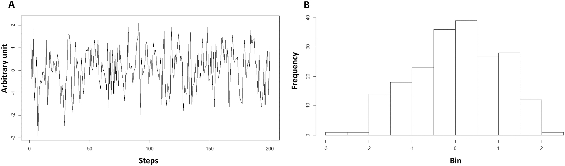
White noise time series A), and its histogram indicating normal distribution B).

Figure 2

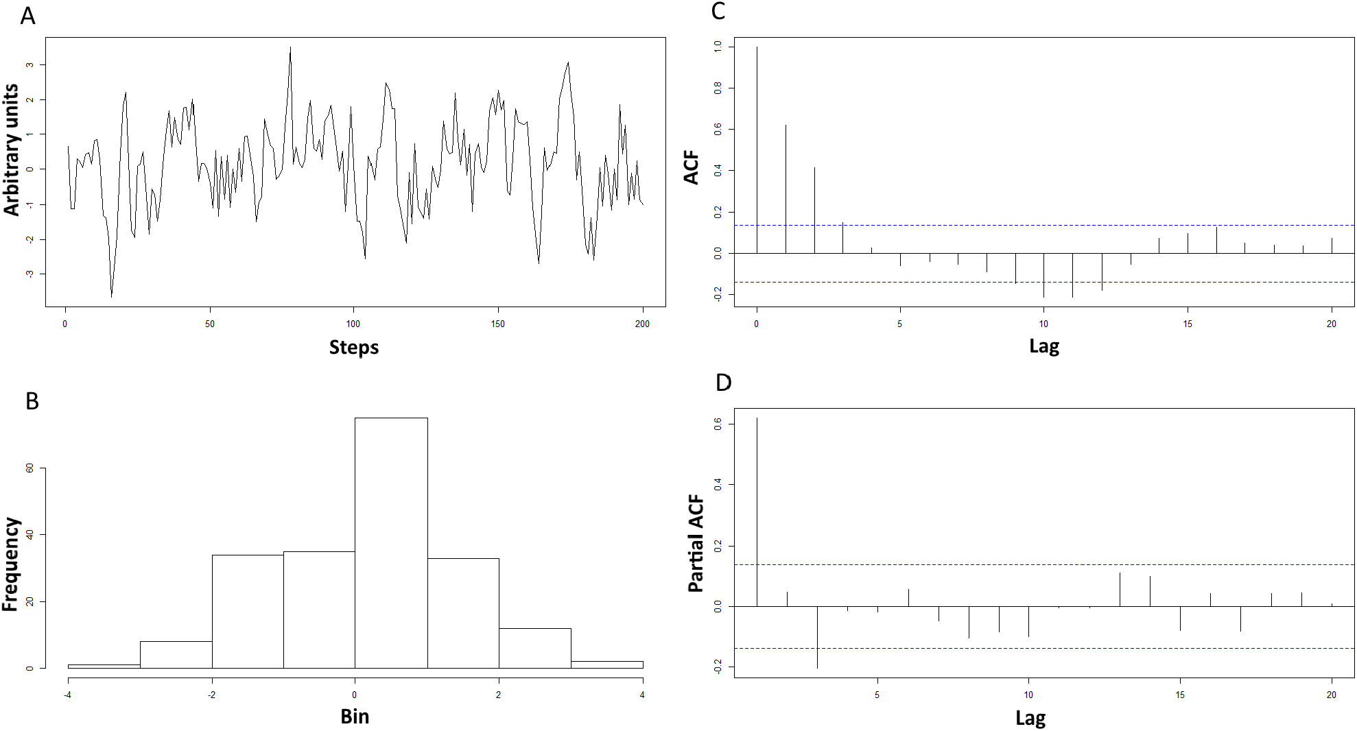
Red noise time series A), its histogram indicating normal distribution B), its autocorrelation function C), and the partial autocorrelation function derived from the series D).

2.1.2 Red noise

The red noise (Figure 2a) was generated by an AR(1) process. The obtained random time series data followed a normal distribution (μ=0.151, σ=1.257), as indicated by the histogram in Figure 2b. The partial autocorrelation function (pACF [45]) confirmed that the generated data came from a first order AR process (ARIMA(1,0,0); Figure 2d).

By fitting an ARIMA(1,0,0) model to the generated red noise time series the parameters of the simulated series were revealed: AR(1)=0.62; intercept=0.15; σ²=0.97; log-likelihood=-280.55; AIC=567.11 [46].

2.1.3 Modification of the generated time series

The last 25% of the time series were modified (from and including the 151^st to the 200^th datum) by (i) adding a constant value (called a “shift”), (ii) adding a trend and (iii) modifying the variance (Figure 3). The modification was commenced using coefficient of variation (CV) based multipliers (m) to ensure relativization of all the modifications, thus facilitating reproducibility (for details see Table 1).

2.2 Breakpoint detection techniques

We hypothesized that the different breakpoint detection methods will be more sensitive to the different modifications, in line with the core of their delineations. Thus, three different types of approach were chosen: one based on primarily detecting change in the first derivative of the trend function of the time series (Section 2.2.1), a second based on a modified cross-entropy method (CE; Section 2.2.2), and a third based on the idea that before and after a breakpoint the distribution of the variable undergoes one or more abrupt change (Section 2.2.3). The methods discussed in the study were chosen based on the facts that these (i) cover the detection of different phenomena, (ii) were published in the last four years and (iii) freely available.

2.2.1 Kink point detection

The method was designed to detect abrupt climate changes with the basic idea of separating trend and noise in the data. The trend describes a temporal change of the expected value which exhibits an abrupt change when the first derivative of the trend function has a discontinuity. Thus, the method indicates a break “kink” point where the continuity of first derivative is obstructed. Decision on trend with kink points against smooth trend, and estimating both the number and locations of these possible points are made employing the generalized cross-validation method. Additionally, a refinement of the methodology is the ability to detect kink points in the temporal changes of the variance, too (for details see [7, 8]).

2.2.2 Multiple Breakpoint Detection via the Cross-Entropy Method (CE)

The Multiple Breakpoint Detection method – implemented in R as a package called ‘ breakpoint ’ [16, 47] – is based on a modified CE approach [48], which is an iterative optimization procedure, yet it is only tuned to detect changes in the mean and not yet in the variance. In every iteration it uses the elite sample (defined by rho) to update the parameters of the sampling distribution. The iteration goes on until a stop criterion (defined by eps) is met (for details see [6]). Specifically, it uses a modified Bayesian Information Criterion [49] to estimate both the number and the corresponding locations of breakpoints. In the present study, due to continuous data the CE. Normal function was used with the distribution set to truncated normal (distyp=2), the maximum number of breakpoints (Nmax) set to five, sample size (M) left as default (200) equal to the total number of observations, and rho=0.25, setting the number of elite samples to 50. All the other options were left as defaults. An additional comment should be made here, namely, that it has been observed that the method is unable to complete the computational task if Nmax> 13.3% of the total number of observations.

2.2.3 Sequential changepoint detection via the CPM Method

The foundations of the Change Point Model (CPM) framework were laid by Hawkins et al. [36], and Hawkins & Zamba [50] to detect changepoints in variance and/or the mean of Gaussian random variables. Numerous CPMs have so far been developed to be applied within this framework to suit the conditions of variously distributed data: parametric, with breakpoints of different origin such as shifts in mean or variance [51], or non-parametric [52], as well. The core of the delineation is that in, e.g. a finite sequence of independent random variables (X₁, •, X_n), where x_t is a particular realization of X_i at the point in time (t_i), the segments before {X₁, •, X_k} and after {X_k+1, •, X_n} a breakpoint (T = k) the distribution of the data is different, and this change can indeed be detected using a two sample hypothesis test [28]. In the present study, since the modelled time series were of Gaussian distribution, the Student-t – tuned for detecting changes in the mean [36] – Bartlett -designed for finding changes in the variance [50] – and Generalized Likelihood Ratio (GLR) statistics – originally tuned for detecting changes in both [51] – were used and compared on the differently modified time series. The Average Run Length (ARL0) – as described in quality control literature [53] – was set to 200, which corresponds to α=0.95, the startup sequence (S) was set to 2,8,10 (corresponding to the default setting 10%=20 pcs. of data) and 32 percent of the total data length and the processStream function was used. S was determined so it would correspond in this study to a certain percentage of the data stream. Generally, regarding S < 10%, the very same breakpoints were estimated. However, the method appeared to be much more successful if the startup sequence was chosen as one third of the total dataset length. Therefore, only those cases are presented in Section 3 in which the method appeared to be the most successful, i.e. S = 32%. The function is tuned to handle a stream of observations and multiple breakpoints. Although only one breakpoint was implemented in the time series, for the sake of comparison with the other methods this was not taken as a known fact. For further details, please see [50].

Table 1.

Table of the applied modifications: the modified value (y) and the value of the original dataset (x) both regarding white and red noise, where m stands for the degree of the modification.

m	Trend, where i = 1 − 50	Shift	Variance
1.5	y=x+i^* 1.5^* CV/100	y=x+CV/10^*1.5	y=x^* CV/10^* 1.5
1	y=x+i^* CV/100	y=x+CV/10	y=x^*CV/10
0.5	y=x+i^* 0.5^* CV/100	y=x+CV/10^*0.5	y=x^* CV/10^* 0.5
0.25	y=x+i^* 0.25^* CV/100	y=x+CV/10^* 0.25	y=x^* CV/10^* 0.25

Figure 3

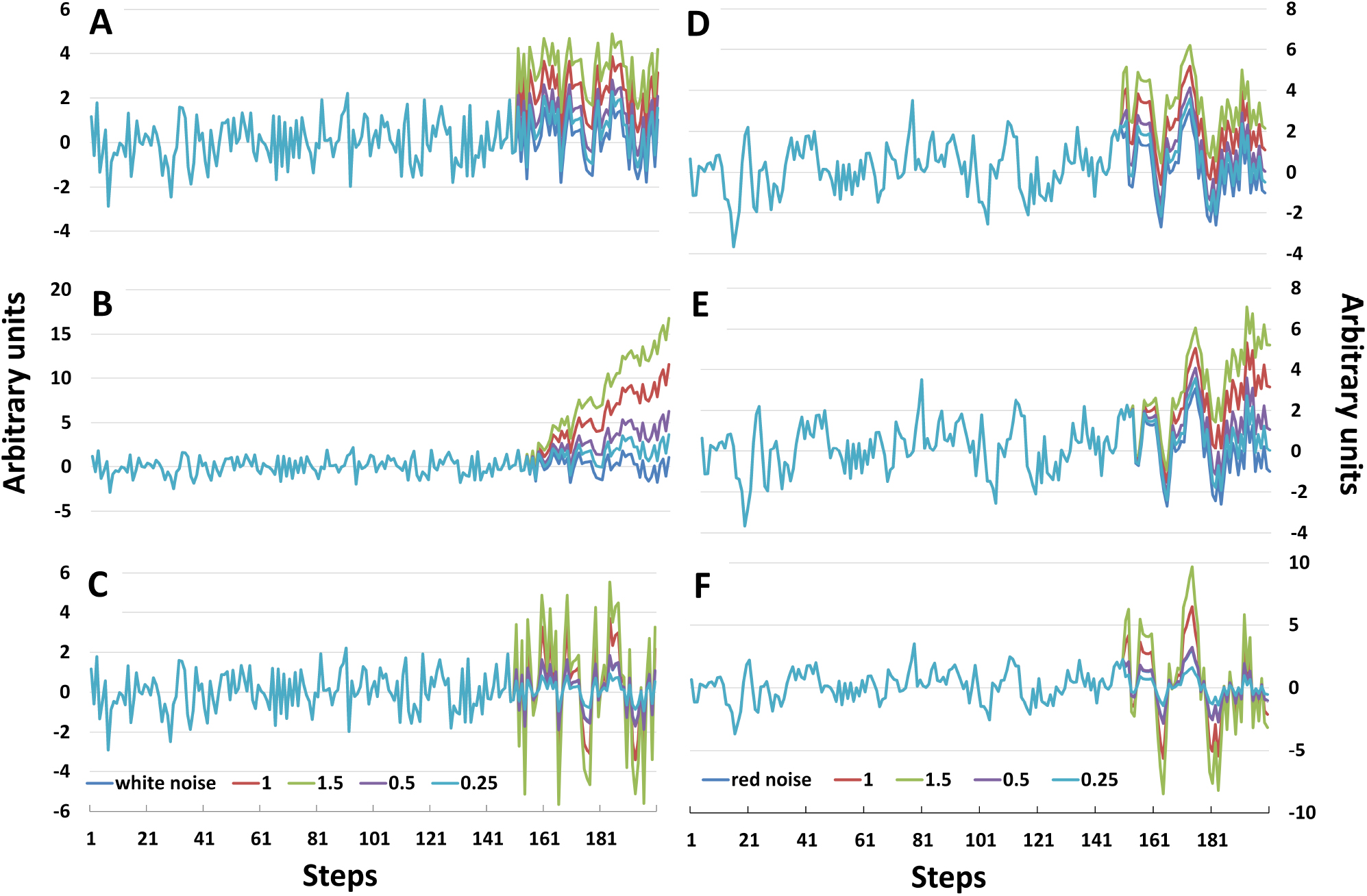
Shift A), trend B), and variance C), modified white noise time series and the shift D), trend E), and variance F) modified red noise time series with the multiplier (m) set to 0.25, 0.5,1 and 1.5.

2.3 Software used

R statistical environment [41] was used to generate the time series and run the calculations using the CE-, [16] and CMP [37] methods, breakpoint, and cpm packages, respectively. The kink point method was applied using our own [7] Fortran code [54].

3 Results

The results show that basically every method is the most applicable if it is a question of finding the breakpoints for which that particular method was designed. However, we also came up against limitations regarding the applicability of the various methods.

As for the modified time series, an ‘acceptance interval’ was introduced. When the detected breakpoints were located at a distance farther than ±5% of the total dataset length from the location of the artificial modifications, the breakpoint was not considered to be accurately found.

3.1 Kink point method

Although, this method was originally designed for detecting trend-type change points, it turned out to be capable of accurately detecting shift-, and variance-type BPs as well. It seems that the location of trend-type modifications is generally over-, while variance-type is under-estimated with this method. As for the shift-type modification, in all cases two BPs were estimated. Another general and important observation is that no BPs were found in the original unmodified datasets.

3.1.1 White noise

Applying the kink point method on trend modified white noise time series all modifications were found with increasing accuracy parallel to the increasing m, with just slight overestimations (Table 2).

With respect to the shift modified datasets (Table 2) BPs were only found if m ≥ 0.5, moreover, not only one, but two BPs were obtained within the acceptance interval. The gap between the two BPs suggests that the kink point detection method handles a shift as two distinct BPs, since this method was originally developed to find discontinuity in the first derivative of the trend function [7]. It is obvious, however, that the smaller the interval between the two BPs, the more accurate the method can be considered.

In the variance modified datasets, BPs were only found if the relative variance of the dataset was increased by at least 100%.

The observations showed that the accuracy of the method is highly dependent on the degree of the implemented modifications; the higher the multiplier, the more accurately were the BPs found with regard to all the three types of modifications (Table 2).

3.1.2 Red noise

In the AR(1) characteristic time series, in general, BPs were found with a slightly lower degree of accuracy than in the white noise ones. The only case with explicit amelioration compared to white noise was at m=1 in the variance modified dataset (BP at 145; Table 2).

Again, the shift modification obliged the kink point method to recognize two BPs located on the two sides of the implemented change. However, the size of the interval between the two BPs was wider than in the case of the white noise time series.

Table 2.

Location (number of data in the sequence) of detected breakpoints by the Kink point method on white and red noise. m stands for the degree of modification. Datasets were modified from the 151^st data.

m	Trend	White noise Shift	Variance	Trend	Red noise Shift	Variance
1.5	152	148;154	145	154	145,158	145
1	154	148;160	140	154	145,158	145
0.5	154	140;160	-	-	-	-
0.25	155	-	-	-	-	-

Table 3.

Location (number of data in the sequence) of detected breakpoints by CE-method with the percentage indicating how many times the particular BP was found. Datasets were modified from the 151^st data, and m stands for the degree of the modification.

m	Trend	White noise Shift	Variance	Trend	Red noise Shift	Variance
1.5	158(10%)	150(45%)	-	146(39%)	147(22%)	-
1	158(16%)	150(47%)	-	146 (47%)	146(57%)	-
0.5	158(32%)	150(82%)	-	147 (100%)	147 (100%)	-
0.25	154(41%)	144 (100%)	-	-(62%)	-(61%)	-

The most important difference arising between the two types of noise was that for white noise, the trend modifications were accurately found, regardless of their degree, even with the smallest multiplier (m=0.25), while in case of red noise this was not true. It was also noticeable that variance-type modifications were not detected when the relative degree of modification was smaller than 100% regarding both white and red noise.

With respect to the kink point detection method it can be said that the best results were obtained with respect to trend-type modifications; however, shift and variance modifications were also accurately located if m ≥ 1.

3.2 CE method

Due to the stochastic characteristics of the CE method [6], its estimates can change slightly from iteration to iteration. Therefore, to get around this problem, the tests were run multiple times, and their distribution was assessed in the course of the analysis. The number of runs (mr) was set to 100 and 200, and with regard to the 3 most frequently occurring BPs, no meaningful difference was observed between the two sets (100; 200). Thus, only the results obtained with mr=100 will be discussed. After assessing the distribution of the obtained breakpoints, so as to better guide the discussion, the location of only the most frequently occurring ones are presented, accompanied by their abundance (%; Table 3). It should be noted here that even according to the authors developing the method, it is not yet able to recognize variance changes [16]. Thus, unsurprisingly, no breakpoints were found in the variance modified time series (Table 3).

In summary, the location of trend-type modifications was overestimated for white noise whereas both trend- and shift-type modifications were underestimated for red noise. It is also important to note that as with the kink point detection method, no BPs were found in the original unmodified datasets here either.

3.2.1 White noise

After having run the analysis on time series characterized by white noise, in the case of trend modified datasets, the located BPs were found to be distributed mainly above the implemented artificial change point, nevertheless still within the acceptance interval (Table 3).

Shift modifications were more accurately estimated than those of trend. The best results (most accurate (150) and highest occurrence (82%)) were obtained if the mean of the original dataset was increased by 50%. In the case of m=0.25, the implemented BP was underestimated.

3.2.2 Red noise

With respect to the datasets characterized by red noise, both trend-, and shift-type modifications were accurately found with high occurrences; they were, however, under-estimated in all cases (Table 3). At m=0.5 for both shift and trend the same BP (147) was found in 100% of the cases, while at m=0.25 in 62 and 61% of the cases, respectively, no BPs were found. In the remainder (38 and 39%) it was falsely estimated to be at the 34^th point.

Regarding the CE method, it can be concluded that (i) it is as yet incapable of handling variance-type BPs, (ii) it is most accurate in locating shift-type BPs in white noise time series, and (iii) in the case of white noise trend-modified processes the locations of BPs are overestimated, while for red noise the opposite is true. Furthermore, the abundance of the most frequently located BPs displays a decreasing tendency with an increasing degree of modification (iv), still giving accurate results, and (v) the most accurate results are obtained if the degree of modification is around 50%.

In time series characterized by AR(1), trend modifications are more successfully located than in the case of AR(0), while regarding shift-type modifications the method appeared to be more accurate when applied to AR(0) time series.

3.3 Change Point Model (CPM) method

All the three test options available for normally distributed data (Student, Bartlett, GLR) were applied on all the modified datasets to reveal the specific discontinuities.

The startup sequence was chosen as 2, 8,10% (10% is same as the default, 20 data points) and 32% of the total length of the data. It was found that under S=10% the exact same output is obtained. The method appeared to be the most successful when the startup sequence was one third of the total dataset length; this way, in most cases only one accurate breakpoint was obtained. It should be noted that during the CPM runs BPs were found in the original unmodified datasets. It therefore had to be tested whether these occurred by chance, or originated from the sensitivity of the CPM method. Thus, a 1000 normally distributed random white and red noise time series were generated without implemented BPs. It was found that in the case of white noise, the Student- and Bartlett tests did not find BPs in about 33%, while GLR did not find any BPs in ∼40% of the time series. In the case of AR(1) type time series, BPs were found technically in almost all cases. Only the Bartlett test was able to produce estimations where no BPs were found in the original unmodified datasets, that is in slightly over 3% of the cases. This phenomenon may presumably be attributed to (i) the sensitivity of the CPM method, and (ii) the fact that it has been developed for datasets with different characteristics than the ones in the present study [50], and this should not therefore be regarded as a “weakness”. Thus, during real-life applications caution is advisable.

Aside from these facts, the accuracy of the CPM method in finding the implemented BPs can indeed be tested, because the BPs found in the original datasets were systematically found in the modified ones as well. However, it is possible to obtain objective results only in those cases where the BPs found in the original dataset were outside the chosen acceptance interval. Therefore, in the following two sections the applicability of the results is restricted to answering the question of whether the different tests found the implemented BPs or not, and to what extent the degree of modification (m) affected these results. In the case of white noise no BPs were found in the original datasets within the acceptance interval, while for red noise this was not true. The Bartlett test on the unmodified data found a BP at the 156^th datum. Therefore, only the Student and GLR test results can only be objectively discussed for red noise.

3.3.1 White noise

Regarding trend modifications, the Student and GLR tests found the exact same BPs regardless of their degree (m) at S=32%. All the BPs were overestimated, and were found inside the acceptance interval, even in the case of the smallest modification (m=0.25). Unsurprisingly, the Bartlett test was only able to find the trend characteristic BPs when the degree of modification was above 50%. In these cases, however, this was accompanied by additional false BPs (Table 4). In the case of S <10%, trend modifications were not found accurately, and the obtained BPs were scattered all over the time series for all three tests. It seems that at S <10%, the artificial BP in the data was recognized as a gradual change (steps) at around the 150^th point.

Shift alternations were accurately found by both Student and GLR tests equally, regardless of the degree of modification. Nonetheless, the smaller the degree of modification, the less accurate BPs were located just as seen previously (Section 3.1). Applying the Bartlett test to shift modified white noise time series no useful results were obtained, since all the BPs were located outside the acceptance interval, along with two pairs already found in the unmodified datasets (Table 4).

It is important to note that variance type alternations were revealed in all cases quite accurately with m ≥100%. With the Bartlett and GLR tests, breakpoints appeared to be accurately located, regardless of the degree of modification, except in cases where the degree of alternation was 50%, in which case, interestingly, no breakpoints were estimated.

It can be concluded that the Student test is the most applicable for detecting shift-type changes, while the Bartlett is successful at recognizing variance-type breaks. The GLR method successfully combines the advantages of these two by detecting changes in both the mean and variance. For trend and shift modifications (which primarily affect the mean), it gave the same BPs as the Student method, while for modifications in the variance, it replicated the Bartlett test results. Trend-type alternations can be estimated most effectively with both Student and GLR tests with S=32%.

3.3.2 Red noise

Breakpoint detection with the CPM method on time series characterized by red noise turned out to be much more challenging than on white noise. As mentioned before, there were cases when BPs were identified in the unmodified datasets. Unfortunately, in case of the Bartlett test, BPs were found in the unmodified time series within the arbitrary chosen acceptance interval (150^th point ±10; ±5% of the total dataset length). Therefore, these test results had to be excluded from the discussion. At the lowest, m=0.25, no meaningful results were obtained.

Trend modifications, taking into account only the results of the Student and GLR tests, did not find BPs within the acceptance interval. Shift type modifications were accurately recognized by the Student and GLR tests only above m=0.5 at the 146^th data point.

In the red noise variance modified time series, only the GLR test was capable of revealing accurate BPs over m=1, with the best result (149 found at m=1.5) for a startup set to 32%. The Student test found one BP for each m=1 and 1.5 just slightly outside the acceptance interval.

In summary, the CPM method was most accurate in the case of shift-type modifications using the Student and the GLR tests, while the Bartlett test (regarding white noise) was most applicable for detecting the variance-type changes.

3.4 Comparison of the test results

The obtained results were compared in detail according to the following criteria: (i/a) how the methods reacted to the different modifications and (i/b) to the change in the multiplier (m) with regard to the accuracy (and in the case of the CE method) and to the abundance of the results, and, (ii) whether any BPs were found in the original, unmodified datasets.

It should again be noted that datasets were modified from the 151^st datum onwards, and there were no BPs placed to the 151^st datum by any of the methods tested (in contrast to placing it at the 150^th). Hence, it can be concluded that the locations indicated by the tests determine the location of the last datum occurring in the sequence before the particular change takes place.

4 Real-life applications

4.1 Application to a historical temperature proxy: vine sprout length data from Hungary

As the timing of life cycle-events recorded in phenological records have been proven to be closely connected to climate variations [55], it becomes more and more important to be able objectively to determine changes in their time series, and thus, hopefully, be able to distinguish between climate-induced and other BPs, as a crucial step before any conclusions are drawn concerning possible climate change.

The Kőszeg (Western Hungary) ‘Book of Vine sprouts’ is a unique collection of life-sized pictorial documents of the vine sprouts with a documented connection to early spring temperatures [56, 57]. Střeštík & Verő [58] were the first to develop a quantitative reconstruction based on this historical phenology evidence. However, after noticing a sharp variance contrast between the 20^th century and the earlier section of the record they tried to eliminate this inhomogeneity by arbitrarily amplifying the variance of the 20^th century part. This would have been a less risky approach if they had omitted either the previous part to their presumed BP or the subsequent part, and/or, preferably, if they had determined the BP in an objective way. The time series was recently reassessed [59], restricting the analysis to only the Burgundy braches – which raises questions not within the scope of the present paper – and determined three BPs (1780; 1820; 1929) using the Bai and Perron multiple breakpoint test [60]. These were subsequently attributed to changes in cultivation/species etc.

We applied the three methods (kink, CE, CPM) so as to determine objectively the suspected BPs. Even a simple visual inspection sheds light on a change in the characteristics of the data passing the midpoint of the record (Figure 4), possibly in variance and mean as well.

Table 4.

Location (number of data in the sequence) of detected breakpoints in white noise modified time series by CPM method (Student, Bartlett and GLR tests). Results outside the chosen accuracy interval (±5% of the total dataset length) are marked with ^*. The underlined BPs were found in the original unmodified datasets as well. Datasets were modified from the 151^st data, m stands for the degree of the modification.

	Trend			Shift			Variance

m	Student	Bartlett	GLR	Student	Bartlett	GLR	Student	Bartlett	GLR
1.5	154	127^*; 152	154	150	127^; 166^	150	154	150	1501
1	154	127^*; 147	154	150	127^{^*}	150	159	150	147
0.5	154	109^; 174^	154	150	46^; 48^	150	-	-	-
0.25	159	109^*	159	154	46^; 48^	154	-	154	154

Table 5.

Location (number of data in the sequence) of detected breakpoints in red noise modified time series detected by the Student and GLR tests of the CPM method. Results outside the chosen accuracy interval (±5% of the total dataset length) are marked with ^*. Only those BPs are listed which were found in the modified datasets. In this case only, the dash (-) means that no other BP was found than the ones in the original datasets. Datasets were modified from the 151^st data; m stands for the degree of the modification.

	Trend		Shift		Variance

m	Student	GLR	Student	GLR	Student	GLR
1.5	130^{^};168^{^}	130^;168^	146	146	161^*	149
1	130^{^};168^{^}	130^;168^	146	146	161^*	146
0.5	-	-	146	146	-	-
0.25	-	-	130^;178^	-	114^;129^;176^*	126^;178^

Table 6.

Summary results of the different BP detection methods on the artificially modified time series.

		Kink	CE	CPM
White noise	Q I/a	Most accurately trend, than shift and lastly variance modifications were found.	Most accurately, trend, than shift was found (method yet incapable of finding variance type BPs).	For Student & GLR most accurately shift, than variance BPs were found. For variance-type BPs Bartlett test was more accurate than GLR.
	I/b	Accuracy increased with m.	Unexpectedly, with m increasing, accuracy decreased along with abundance.	Accuracy increased with m
	QII	None found in the original data.	None found in the original data.	Limited.
Red noise	Q I/a	No pronounced difference between the different modifications		For trend no meaningful result was obtained. For shift, Student- & GLR produced similar accuracy and to find variance type of BPs GLR is the best solution.
	I/b	m ≥ 1, no meaningful difference observed.	m ≥ 0.5, no meaningful difference in accuracy and abundance observed.	-
	QII	None found in the original data.	None found in the original data.	Numerous BPs found in all cases.

The Kink point method was not able to identify any breakpoints in the vine sprout length data, which forecasted that the awaited structural change in the data could not be of the trend type. This hypothesis was further enforced by the other two methods, since those are sensitive to other types of structural change, such as mean and/or variance, and not trend.

The CE method was run 100 times with the same parameters as on the artificial data (Section 2.2.2). The results indicated that most probably one BP exists in the time series, and it is very likely the year 1907, corresponding to the 120^th data point, since 75% of the detected BPs were placed there (Figure 4). In the remaining 25% of the cases, it was estimated to be at the 112^th data point, corresponding to 1899.

As for the CPM results, all three tests were run, supplemented by a fourth, nonparametric one (Mann-Whitney), tuned to locate shifts. These identified numerous BPs. However, having compared these to each other, only two breakpoints were indicated by multiple tests: 119/120 and 201, corresponding to the years 1906/7 and 1988 (Table 7).

Interestingly, neither of the BPs found by the two methods (CE & CPM; Table 7) match those reported by Parisi et al. [59], which raises concerns about their interpretations. However, it should be noted that the datasets used [59] differed slightly from that used in the present study. Parisi et al. [59] re-measured the pictures in the ‘Book of Vine sprouts’, while we used the data published by Strestik & Vero [58] and omitted the values before 1788, so no gaps would occur.

Nevertheless, the BPs placed at the turn of the 20^th century (Table 7) coincided with previous suppositions [58]. The BP found in 1899 matched exactly the first occurrence of the phylloxera disease in the Kőszeg area, which caused a complete change in the species composition of the vineyards [61]. This change had presumably affected viticulture to such an extent that after 1908 the population cannot be further considered as homogeneous. The results may be considered important from several paleoclimatological points of view: in a recent study, for example, because the CPM placed the BP to 1906 and the CE to 1907, the data after 1906 was omitted for spring temperature reconstructions [57].

From the observations of the artificial time series (Table 6) and the results seen above, it can also be concluded that the BP found at the 119/120^th data point is of the shift type, while at datum 201 it may be presumed to be a variance type of change, though the restricted number of data after the BP makes it difficult to decide.

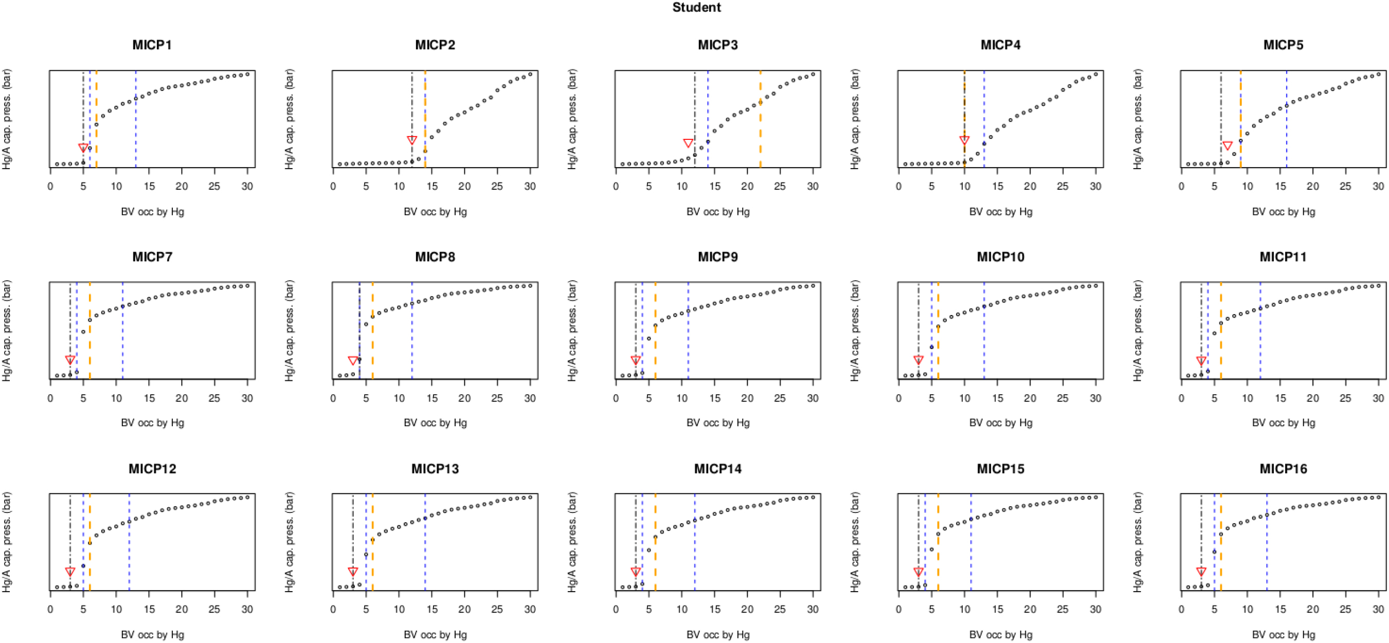
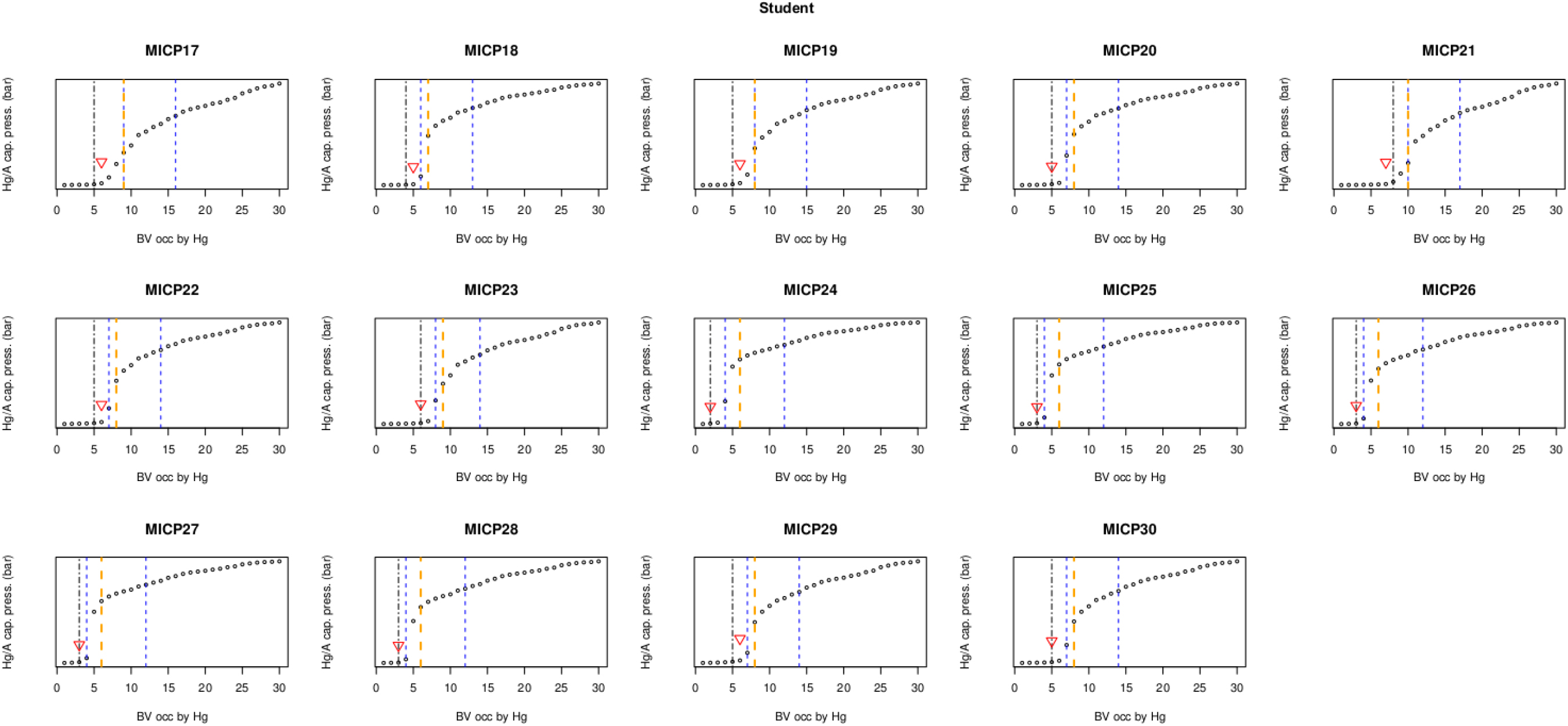
4.2 Application to the closure-correction of mercury-injection capillary-pressure (MICP) curves

In petrophysical analyses, mercury drainage capillary pressure curves serve as a vital stepping-stone in the determination of initial fluid distribution in the subject reservoir rock and thus in determining the efficiency with which a non-wetting phase can be taken from a pore system [62]. In general practice, the raw drainage capillary pressure curves’ assessment starts with the fitting of two linear trends on the data and the discarding of the shorter segment (i.e. closure correction). With the residuals’ capillary curve, a Thomeer evaluation [63] can be conducted, describing the residual curve with a hyperbola. However, closure correction is performed manually, based on the expert’s professional experience (that is, arbitrarily).

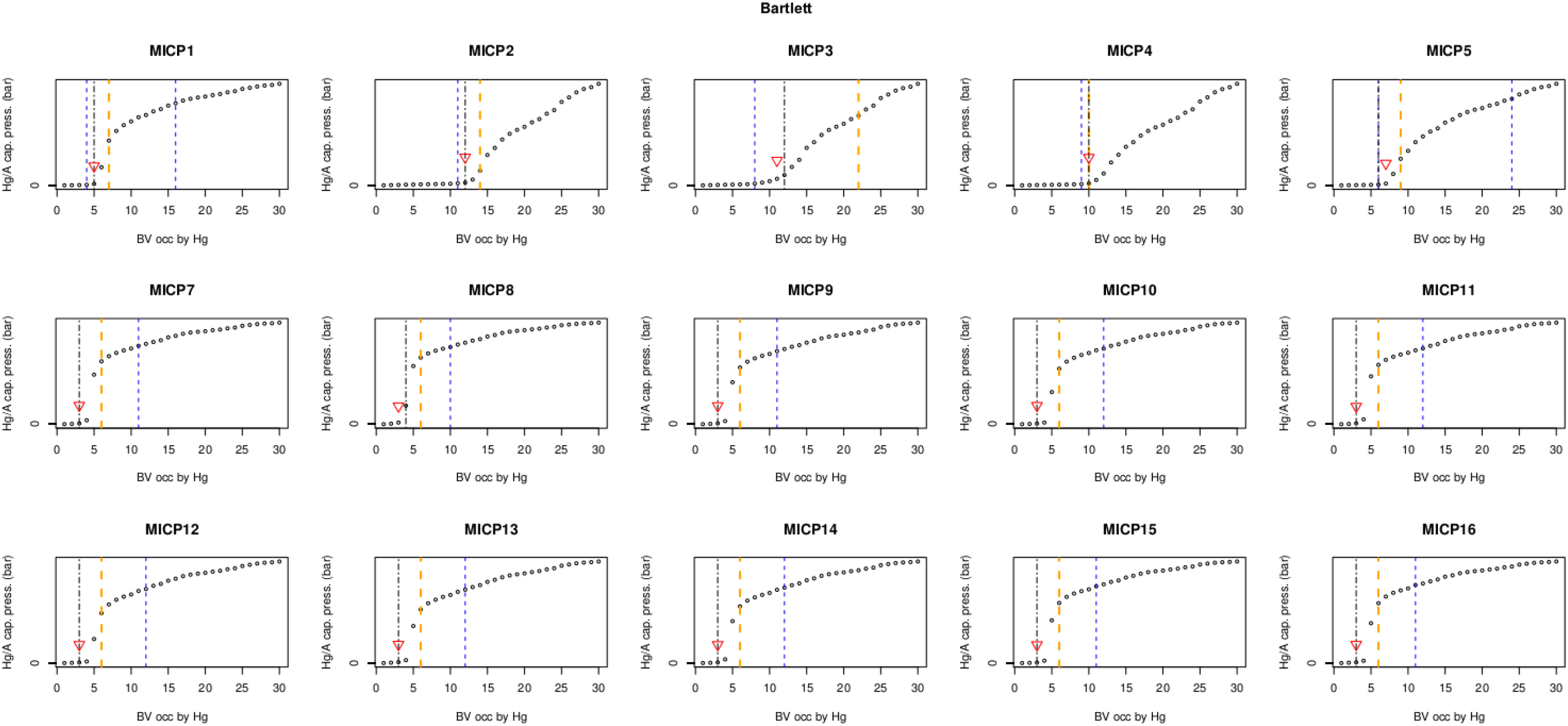
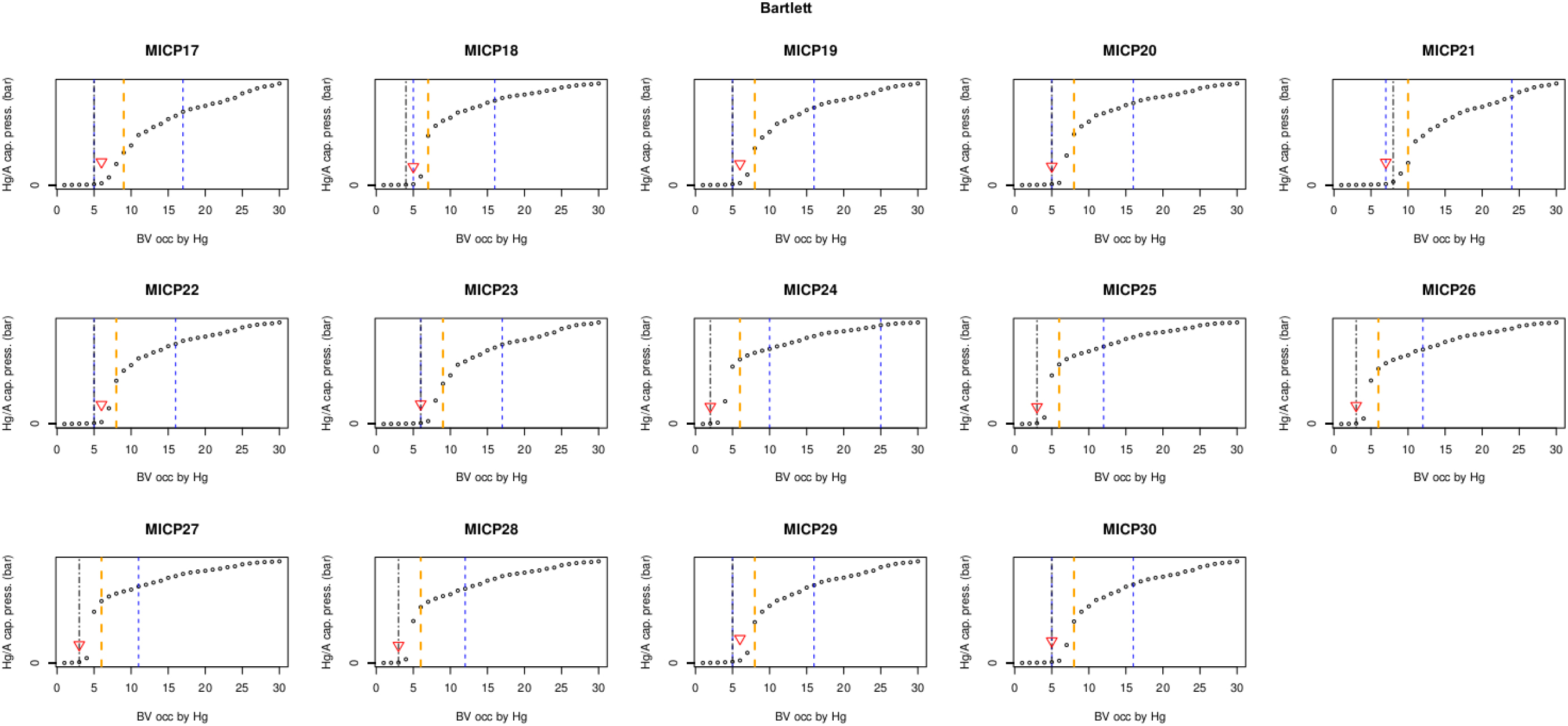
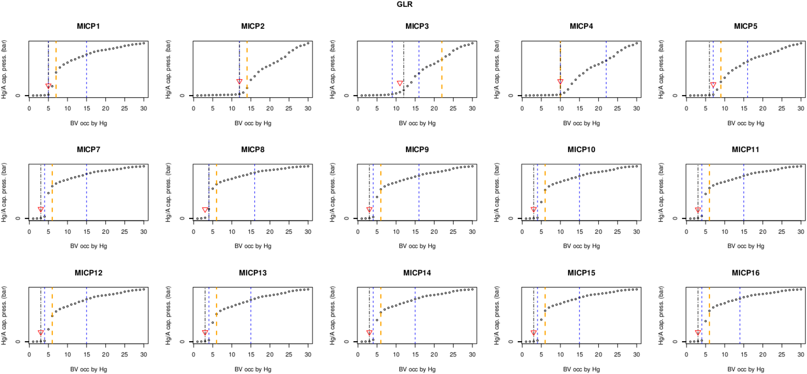
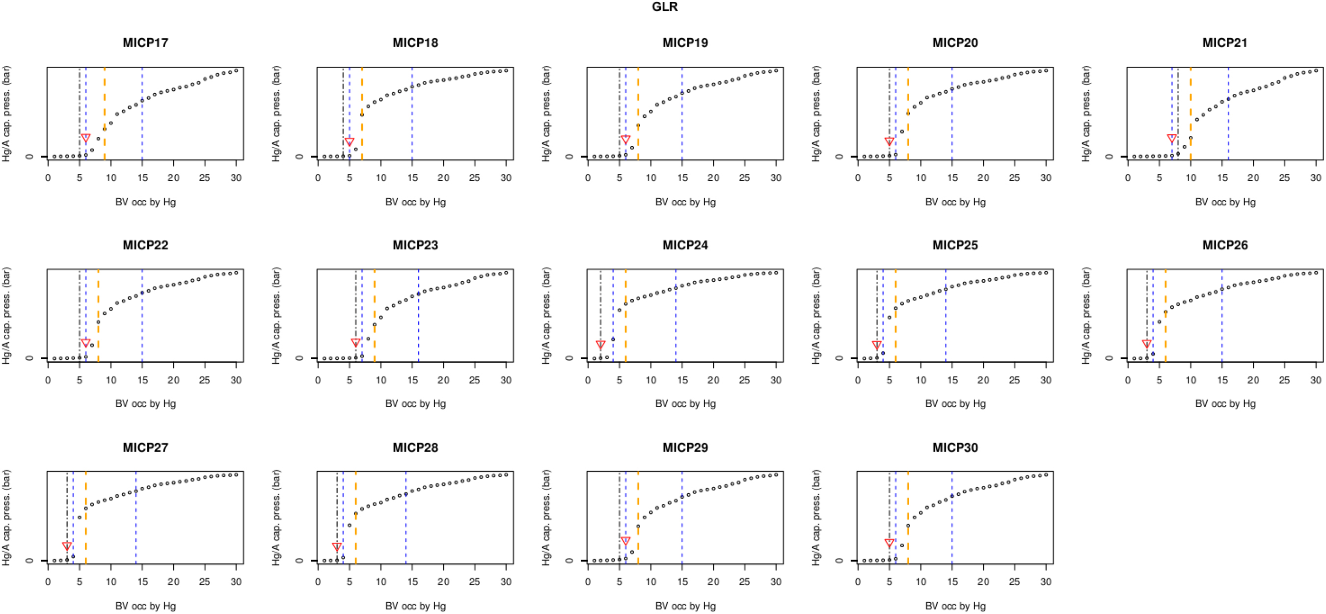
Through the application of the three BP detection methods at hand (kink point, CE and CPM) on the 29 available MICP curves [64], it became possible to validate the expert’s decision and, vice-versa, to evaluate the methods’ efficiency. In the analysis, the values indicating the location of the BPs determined by the expert correspond to the last datum which was discarded. Thus, the break is between the value pointed out as the BP and the following one.

First, the BPs were determined using each method (for details see the Appendix) and then the differences between those and the locations of the BPs determined by the expert were computed and summarized (Table 8).

It can be concluded that in order of decreasing accuracy the kink point, GLR, Student, CE and the Bartlett methods were capable of finding BPs closest to those identified by the expert. The average difference between the expert’s evaluations and the breakpoints found by the kink point method was μ= -0.10, with a standard deviation of σ = 0.56. The tendency was to overestimate the BPs, and the few cases when underestimation was observed belonged mainly to those indicated by the Bartlett and kink point methods (15 out of the 16 underestimations; Table 8).

In summary, the kink point method was shown to be the most suitable to facilitate the industrial task of assessing the closure-correction of MICP curves, and its application would indeed accelerate the process, freeing up human resources.

Figure 4

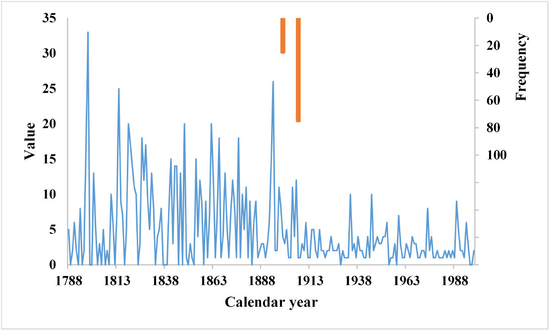
Vine sprout length data A) and the distribution of BPs found using the CE method in the gapless period (1788-1998) B).

Table 7.

BPs found in the vine sprout data using the CPM & the CE method. The BPs found by at least three methods/tests are highlighted.

	CPM			CE
MW	GLR	Bartlett	Student
25	49	14	119	112(25%)
45	51	55	201	120(75%)
119	98	57
	104	98
	126	104
	128	126
	151	128
	153	146
	155	167
	173	169
	175	189
	189	191
	191	201
		201

Table 8.

Descriptive statistics of the differences between the location of the BPs found by the expert and the different methods on the 29 MICP curves. Negative values indicate under-, while positive ones overestimation. The statistics were computed using only the most frequently found CE BPs (average abundance was 33.7%). Data was obtained from Nemes [61].

	CPM
	Kink point	GLR	Student	Bartlett
Min.	−1.00	−2.00	1.00	−3.00	0.00
Max.	1.00	2.00	3.00	9.00	11.00
Med.	0.00	1.00	2.00	7.00	3.00
St.dev.	0.56	0.73	0.72	4.76	1.70
Avg.	−0.10	0.59	1.66	4.00	2.97

5 Conclusions and outlook

By comparing the sensitivity of three breakpoint detection techniques, their basic differences were highlighted. The results draw attention to the fact that the detection of breakpoints is indeed dependent on the degree and type of the modifications and the computational background of the detection methods. Most importantly: (i) the CE & kink point methods did not find any breakpoints in the original dataset, unlike the CPM method (probably due to its basic sensitivity), (ii) breakpoints in AR(0) time series are handled more successfully, and (iii) the most explicit amelioration in accuracy was witnessed starting from m > 0.5. As seen in recent studies, with multiple methods applied together [29], the suspected breakpoints can be more effectively found. In the present study, the information gained from the test on artificial breakpoints and those documented in literature were combined.

On the one hand, documented BPs were verified, while others were questioned in a historic grape phenology dataset; on the other hand, the practice of closure-correction of MICP curves was facilitated and expedited, sparing human resources and leading towards a more objective industrial practice. The interpretation of real life data sets was supported by the experience gained from the “artificial” exercises.

Acknowledgement

Support for this work was provided by the MTA “Lendület” program (LP2012-27/2012). This is contribution No. 30 of 2ka Paleoclimatology Research Group.

References

1 Tsay R.S., Outliers, level shifts, and variance changes in time series, J. Forecasting, 1988, 7, 1-20.10.1002/for.3980070102Suche in Google Scholar

2 Hamed K.H., Rao A.R., A modified Mann-Kendall trend test for autocorrelated data, J. Hydrology, 1998, 204,182-196.10.1016/S0022-1694(97)00125-XSuche in Google Scholar

3 Meehl G.A., Karl T., Easterling D.R., Changon S., Pielke R. Jr., Chagnon D. et al., An introduction to trends in extreme weather and climate events: observations, socioeconomic impacts, terrestrial ecological impacts, and model projections, Bull. Amer. Meteor. Soc., 2000, 81, 413-416.10.1175/1520-0477(2000)081<0413:AITTIE>2.3.CO;2Suche in Google Scholar

4 Karl T.R., Knight R.W., Baker B., The record breaking globaltemperatures of 1997 and 1998: Evidence for an increase in the rate of global warming?, Geophys. Res. Lett., 2000, 27(5), 719-722.10.1029/1999GL010877Suche in Google Scholar

5 Tomé A.R., Miranda P.M.A., Piecewise linear fitting and trend changing points of climate parameters, Geophys. Res. Lett., 2004, 31, L02207.10.1029/2003GL019100Suche in Google Scholar

6 Priyadarshana W.J.R.M., Sofronov G., Multiple Breakpoints Detection in array CGH Data via the Cross-Entropy Method, IEEE/ACM Trans. Comput. Biol. Bioinf., 2015, 12(2), 487-498.10.1109/TCBB.2014.2361639Suche in Google Scholar

7 Matyasovszky I., Detecting abrupt climate changes on different time scales, Theor. Appl. Climatol., 2011,105, 445-454.10.1007/s00704-011-0401-4Suche in Google Scholar

8 Matyasovszky I., Ljungqvist F.C., Abrupt temperature changes during the last 1,500 years, Theor. Appl. Climatol., 2012, 112, 215-225.10.1007/s00704-012-0725-8Suche in Google Scholar

9 Wang G., Xia J., Chen J., Quantification of effects of climate variations and human activitieson runoff by a monthly water balance model: A case study of the Chaobai River basin in northern China, Water Resour. Res., 2009, 45, W00A11.10.1029/2007WR006768Suche in Google Scholar

10 He W.P., Feng G.L., Wu Q., Wan S.Q., Chou J.F., A new method for abrupt change detection in dynamic structures, Nonlin. Proces. Geophys., 2008, 15, 601-606.10.5194/npg-15-601-2008Suche in Google Scholar

11 McCarthy M.P., Titchner H.A., Thorne P.W., Tett S.F.B., Haimberger L., Parker D.E., Assessing bias and uncertainty in the HadAT-Adjusted radiosonse climate record, J. Climate, 2007, 21, 817-832.10.1175/2007JCLI1733.1Suche in Google Scholar

12 Davis R.A., Lee T.C.M., Rodrigez-Yam G.A., Structural break estimation for nonstationary time series models, JASA, Theory and Methods, 2006, 101(473), 223-239.10.1198/016214505000000745Suche in Google Scholar

13 Lindau R., Venema V., On the multiple breakpoint problem and the number of significant breaks in homogenization of climate records, Időjäräs, OMSZ, 2013,117(1), 1-34.Suche in Google Scholar

14 Jinwen Z., Jie M., Measurement for the breakpoints and transition functions for monetary policy operation of China’s Center Bank, Economic Research Journal, 2005, 12, 009.Suche in Google Scholar

15 Ross G.J., Modelling financial volatility in the presence of abrupt changes, Physica A, 2012, 392(2), 350-360.10.1016/j.physa.2012.08.015Suche in Google Scholar

16 Priyadarshana W.J.R.M., Sofronov G., A Modified Cross-Entropy Method for Detecting Multiple Change-Points in DNA Count Data, In Proc. of the IEEE Conference on Evolutionary Computation (CEC), 2012,1020-1027.10.1109/CEC.2012.6256470Suche in Google Scholar

17 Jong K., Marchiori E., Vaart A.V.D., Ylstra B., Weiss M., Meijer G., Chromosomal breakpoint detection in human cancer, Applications of evolutionary computing lecture notes in Computer Science, 2003, 2611, 54-65.10.1007/3-540-36605-9_6Suche in Google Scholar

18 Bakhshi A., Jensen J.P., Goldman P., Wright J.J., McBride O.W., Epstein A.L. et al., Cloning the chromosomal breakpoint of t(14;18) human lymphomas: clustering around JH on chromosome 14 and near a transcriptional unit on 18, Cell, 1985, 41, 899-906.10.1016/S0092-8674(85)80070-2Suche in Google Scholar

19 Varotsos P., Lazaridou M., Latest aspects of earthquake prediction in Greece based on seismic electric signals, Tectonophysics, 1991,188(3-4), 321-347.10.1016/0040-1951(91)90462-2Suche in Google Scholar

20 Varotsos P.A., Sarlis N.V., Skordas E.S., Detrended fluctuation analysis of the magnetic and electric field variations that precede rupture, Chaos, 2009,19, 023114.10.1063/1.3130931Suche in Google Scholar PubMed

21 Varotsos P.A., Sarlis N.V., Skordas E.S., Lazaridou M.S., Fluctuations, under time reversal, of the natural time and the entropy distinguish similar looking electric signals of different dynamics, J. Appl. Phys., 2008,103, 014906.10.1063/1.2827363Suche in Google Scholar

22 Varotsos P.A., Sarlis N.V., Skordas E.S., Long-range correlations in the electric signals that precede rupture: further investigations, Phys. Rev. E, 2003, 67, 021109.10.1103/PhysRevE.67.021109Suche in Google Scholar PubMed

23 Varostos P., Sarlis N.V., Skordas E.S. et al., Natural time analysis of critical phenomena, PNA, 2011,108(28), 11361-11364.10.1073/pnas.1108138108Suche in Google Scholar PubMed PubMed Central

24 Williams S.D.P., Offsets in Global Positioning System time series, J. Geophys. Res., 2003, 108(B6), 2310.10.1029/2002JB002156Suche in Google Scholar

25 Gazeaux J., Williams S., King M., Bos M., Dach R., Deo M., Moore A.W., Ostini L., Petrie E., Roggero M., Teferle F.N., Olivares G., Webb F.H., Detecting offsets in GPS time series: first results from the detection of offsets in GPS experiment. J. Geophys. Res. Solid Earth, 2013, 118(5), 2397-2407.10.1002/jgrb.50152Suche in Google Scholar

26 Manley G., Central England temperatures: Monthly means 1659 to 1973., Q.J.R. Meteorol. Soc., 1974,100(425), 389-405.10.1002/qj.49710042511Suche in Google Scholar

27 Lindau R., Venema V., The uncertainty of break positions detected by homogenization algorithms in climate records, Int. J. Climatol., 2015, D0I:10.1002/joc.4366.10.1002/joc.4366Suche in Google Scholar

28 Shirvani A., Change point analysis of mean annual air temperature in Iran, Atmos. Res., 2015, 160, 91-98.10.1016/j.atmosres.2015.03.007Suche in Google Scholar

29 Haidu I., A stochastic vision of the paleoclimate. Modeling and predictability. In: Late Pleistocene and Holocene Climatic Variability in the Carpathian-Balkan Region, Stefan cel Mare University Press, Suceava, Romania, 2014.Suche in Google Scholar

30 Costa A.C., Soares A., Homogenization of climate data: review and new perspectives using geostatistics, Math. Geosci., 2009, 41(3), 291-305.10.1007/s11004-008-9203-3Suche in Google Scholar

31 Kuglitsch F.G., Auchmann R., Bleisch R., Brönnimann S., Martius O., Stewart M., Break detection of annual Swiss temperature series, J. Geophys. Res., 2012, 117, D13105.10.1029/2012JD017729Suche in Google Scholar

32 Omumbo J.A., Lyon B., Waweru S.M., Connor S.J., Thomson M.C., Raised temperatures over the Kericho tea estates: revisiting the climate in the East African highlands malaria debate, Malar. J., 2011, 10(12), D0I:10.1186/1475-2875-10-12.10.1186/1475-2875-10-12Suche in Google Scholar PubMed PubMed Central

33 Zimmerman D.W., Comparative power of Student T test and Mann-Whitney U test for unequal sample sizes and variances, J. Exp. Edu., 1987, 55(3), 171-174.10.1080/00220973.1987.10806451Suche in Google Scholar

34 Wang J., Zivot E. A Bayesian time series model of multiple structural changes in level, trend and variance, J. Bus. Econ. Stat., 2000, 18, 3.10.1080/07350015.2000.10524878Suche in Google Scholar

35 Topal D., Hatvani I.G., Matyasovszky I., Kern Z., Break-point detection algorithms tested on artificial time series, In: Janina Horvath, Marko Cvetkovic, Istvan Gabor Hatvani (szerk.): 7th Croatian – Hungarian and 18th Hungarian Geomathematical Congress: “The Geomathematical Models: The Mirrors of Geological Reality or Science Fictions?”. Conference venue: Mórahalom, Hungary 21-23.05.2015, Hungarian Geological Society, 2015, 147-154.Suche in Google Scholar

36 Hawkins D.M., Qiu P., Kang C.W., The Changepoint Model for Statistical Process Control, J. Quality Technology, 2003, 35(4), 355-366.10.1080/00224065.2003.11980233Suche in Google Scholar

37 Ross G.J., Parametric and Nonparametric Sequential Change Detection in R: The cpm Package, J. Stat. Softw., 2015.10.18637/jss.v066.i03Suche in Google Scholar

38 Franke J., Frank D., Raible C.C., Esper J., Brönnimann S., Spectral biases in tree-ring climate proxies, Nat. Clim. Chang., 2013, 3, 360-364.10.1038/nclimate1816Suche in Google Scholar

39 Vasseur D.A., Yodzis P., The color of environmental noise, Ecology, 2004, 85(4), 1146-1152.10.1890/02-3122Suche in Google Scholar

40 Pelletier J.D., Turcotte D.L., Long-range persistence in climatological and hydrological time series: analysis, modelling and application to drought hazard assessment, J. Hydrology, 1997, 203, 198-208.10.1016/S0022-1694(97)00102-9Suche in Google Scholar

41 R Core Team, R: A Language and Environment for Statistical Computing, R Foundation for Statistical Computing, Vienna, Austria. 2008, ISBN 3-900051-07-0, URL http://www.R-project.org.Suche in Google Scholar

42 Kovacs J., Markus L., Szalai J., Kovacs I.S., Detection and evaluation of changes induced by the diversion of River Danube in the territorial appearance of latent effects governing shallow ground water fluctuations, J. Hydrology, 2015, 520, 314-325.10.1016/j.jhydrol.2014.11.052Suche in Google Scholar

43 Markus L., Berke O., Kovacs J., Urfer W., Spatial Prediction of the Intensity of Latent Effects Governing Hydrogeological Phenomens, Environmetrics, 1999,10(5), 633-654.10.1002/(SICI)1099-095X(199909/10)10:5<633::AID-ENV378>3.0.CO;2-8Suche in Google Scholar

44 Matyasovszky I. Meteorológiai idősorok modellezése ARMA folyamatoksegitségével, PhD Thesis, Eötvös Lorand University, Faculty of Meteorology, Budapest, 1986 (In Hungarian).Suche in Google Scholar

45 Box G.E.P., Jenkins G.M., Reinsel G.C., Time Series Analysis, Forecasting and Control, NJ: Prentice Hall, Englewood Cliffs, 1994.10.1002/9781118619193Suche in Google Scholar

46 Akaike H., A new look at the statistical model identification (PDF), IEEE Trans. Autom. Control, 1974, 19(6), 716-723.10.1109/TAC.1974.1100705Suche in Google Scholar

47 Priyadarshana W.J.R.M., Sofronov G., The Cross-Entropy Method and Multiple Change-Points Detection in Zero-Inflated DNA read count data, In: Y.T. Gu, S.C. Saha (Eds.) The 4th International Conference on Computational Methods (ICCM2012), 2012, 1-8, ISBN 978-1-921897-54-2.Suche in Google Scholar

48 Evans G.E., Sofronov G., Keith J.M., Kroese D.P., Identifying change-points in biological sequences via the cross-entropy method, Ann. Oper. Res., 2011,189(1), 155-165.10.1007/s10479-010-0687-0Suche in Google Scholar

49 Zhang N.R., Siegmund D.O., A modified Bayes information criterion with applications to the analysis of comparative genomic hybridization data, Biometrics, 2007, 63, 22-32.10.1111/j.1541-0420.2006.00662.xSuche in Google Scholar

50 Hawkins D.M., Zamba K.D., A Change-Point Model for a Shift in Variance, JQT, 2005, 37(1), 21-31.10.1080/00224065.2005.11980297Suche in Google Scholar

51 Hawkins D.M., Zamba KD., Statistical Process Control for Shifts in Mean or Variance Using a Change point Formulation, Technometrics, 2005, 47(2), 164-173.10.1198/004017004000000644Suche in Google Scholar

52 Ross, G.J., Tasoulis, D.K., Adams N.M., Nonparametric Monitoring of Data Streams for Changes in Location and Scale, Technometrics, 2011, 53(4), 379-389.10.1198/TECH.2011.10069Suche in Google Scholar

53 Fu J.C., Spiring F.A., Xie H., On the average run lengths of quality control schemes using a Markov chain approach, Statist. Probab. Lett., 2002, 56, 369-380.10.1016/S0167-7152(01)00183-3Suche in Google Scholar

54 Backus J., The history of Fortran I, II, and III, History of programming languages I. ACM, 1978,13(8), 165-180.10.1145/960118.808380Suche in Google Scholar

55 Vliet V.A.J.H., Schwartz M.D., Phenology and climate: the timing of life cycle events as indicators of climatic variability and change, Int. J. Climatol. 2002, 22(14), 1713-1714.10.1002/joc.816Suche in Google Scholar

56 Berkes Z., ÉghajlatingadozàsoktUkrozó’dése a koszegiszolohajtasok hosszaban / Spiegelung der Klimaschwankungen in dem Längenwachstum der Weinreben-Triebe in Kőszeg, Magyar Kiralyi Orszagos Meteorológiai és Földmâgnességi Intézet, Budapest, Hungary, 1942 (in Hungarian and German).Suche in Google Scholar

57 Kern Z., Németh A., Gulyás M.H., Popa I., Levanič T., Hatvani I.G., Natural proxy records of temperature- and hydroclimate variability with annual resolution from the Northern Balkan-Carpathian region for the past millennium – review & recalibration, Quaternary International, 2016 (in press) DOI:10.1016/j.quaint.2016.01.012.10.1016/j.quaint.2016.01.012Suche in Google Scholar

58 Střeštík J. Verő J., Reconstruction of the spring temperatures in the 18th century based on the measured lengths of grapevine sprouts, Időjârâs, 2000, 104, 123-136.Suche in Google Scholar

59 Parisi S.G., Antoniazzi M.M., Cola G., Lovat L. et al., Spring thermal resources for grapevine in Kőszeg (Hungary) deduced from a very long pictorial time series (1740-2009), Climatic Change, 2014, 126, 443-454.10.1007/s10584-014-1220-2Suche in Google Scholar

60 Bai J., Perron P., Estimating and testing linear models with multiple structural changes, Econometrica, 1998, 66(1), 47-78.10.2307/2998540Suche in Google Scholar

61 Bariska I., A koszegi bor, Escort 96 BT, Sopron, Hungary, 2001 (In Hungarian).Suche in Google Scholar

62 Wardlaw N.C., Taylor R.P., Mercury capillary pressure curves and the interpretation of pore structure and capillary behaviour in Reservoir Rocks, Bulletin of Canadian Petroleum Geology, 1976, 24(2), 225-262.Suche in Google Scholar

63 Thomeer J.H.M., Introduction of a Pore Geometrical Factor Defined by the Capillary Pressure Curve, JPT, 1960,12(03), 73-77.10.2118/1324-GSuche in Google Scholar

64 Nemes I., Revisiting the applications of drainage capillary pressure curves in water-wet hydrocarbon systems, Open Geosci., 2016 (in press), DOI:10.1515/geo-2016-0007.10.1515/geo-2016-0007Suche in Google Scholar

A Appendix Detecting breakpoints in artificially implemented and real-life time series using state-of-the-art methods

The following graphs represent the breakpoints found by the Expert (red triangle pointing down), found by the specific test of the CPM method (blue broken vertical line), the CE method (thick orange broken vertical line) and the Kink point method (black broken and dotted vertical line). The measurement unit of capillary pressure for Hg/Air is in bars, however the axis has been rescaled arbitrarily.