Redistricting for Proportionality

1 Introduction

Most American legislative elections are plurality contests in single-member districts, a system we will abbreviate by PSMD: the single candidate with the most votes is elected from each geographical district. This stands in contrast to much of the rest of the world, where legislatures are filled by a mechanism that has proportionality guarantees by design, such as a “party list” system that awards seats to political parties in proportion to their vote share. The positive case for PSMD as a system centers on the importance of local and regional choice, with voters directly choosing their representatives; PSMD offers the prospect that preferences that are in the minority on a statewide level can secure majority support in a smaller geography. However, it has long been observed that actual PSMD elections are routinely disproportional, and recent years have seen increasingly sophisticated modeling that shows that even blind PSMD—via randomized legally valid districts—is disproportional in ways that are unpredictable from state to state, because they depend on the precise spatial arrangement of vote preferences. Nevertheless, public perceptions of fair outcomes remain closely tied to proportionality, i.e. the degree of congruence between vote share and seat share. In this paper, we consider whether PSMD can be made compatible with a fairness norm calling for proportional outcomes. That is, it possible to counteract the central tendencies of party-blind districting and to expressly design districts that are likely to produce proportional representation?^[1] Below, we address this question in highly practical terms, by considering how a test of gerrymandering could be administered in law, via the “FTV Test” set down in draft Congressional legislation in 2021.

That is, suppose a state were to adopt partisan proportionality as a goal in its law or guidelines for redistricting, reflecting a preference for a plan that is likely to elect a delegation with each party’s seat share approximating its vote share. Indeed, one state—Ohio—has proportionality written into its state constitution as a policy goal.^[2] Is that a feasible goal for mapmakers? Or is this an unattainable goal—and therefore an unreasonable legal standard?

After regaining control of both houses of Congress in 2021, Democratic lawmakers attempted several times to pass a bill that would address redistricting. In particular, they sought to rein in partisan gerrymandering in the wake of the 2019 Rucho v. Common Cause Supreme Court decision that declared it non-justiciable in federal courts. Here is the proposed test from Senate Bill 2747, the “Freedom to Vote: John R. Lewis Act” (S.2747 – Freedom to Vote Act 2747), paraphrased succinctly. We will call it the FTV Test (See Appendix B for full text.)

According to a recognized metric of partisan fairness, a plan must yield nearly (within a set tolerance) the ideal /target seat share for each party in at least three out of a prescribed list of four recent elections.

The metric that sets the target was left unspecified, as we explore below, but the four elections were designated in the bill to be the two most recent contests for President and for U.S. Senate. If the test is failed—i.e. if the tolerance is exceeded in two or more of the four contests—this triggers a presumption that the plan is gerrymandered, which can then be rebutted by the state. But as an initial matter, this is an unabashedly simple and results-based (not intent-based) test.

In this paper we consider what kinds of fairness metrics are potentially suitable for use in the test, first discussing them in normative terms. Circling back to the motivating question above, we focus on the viability of using the FTV Test with a proportionality target. We focus on five states that had extensive legal challenges with a partisan gerrymandering component circa 2018: North Carolina (challenged in federal and state court), Maryland (federal), Pennsylvania (state), Texas (federal), and Wisconsin (federal).^[3] We add Massachusetts, which is known to have a very uniform political geography, making the state a hard case for many fairness norms, as we will see below. We are armed with large collections of alternative districting plans generated by computer as well as alternative plans drawn by courts and journalists, and we use contemporaneous election data from the period preceding 2018. We will demonstrate that in the contested states, mapmakers can reasonably produce examples that satisfy the FTV Test for proportionality, suggesting that the test is not too stringent. Massachusetts give us an example where proportionality is out of reach, and is used here to illustrate that the FTV test handles that case well with the rebuttal element in its design. But of course this proposed policy aims to validate plans for adoption that are likely to retain their good properties into the future. This leads us to investigate whether plans that are near-proportional in an earlier election window will tend to remain so in subsequent years. The findings there are encouraging as well.

2 Proportionality and Other Ideals

2.1 Norms of Fairness

By design, the FTV Test leaves open an obvious question—what is the ideal seat share? Several possibilities might be considered. Let us denote by V the statewide share of the (major-party) vote that belongs to a political party, and by S their share of representation, for a given vote pattern and districting plan.

2.1.1 Normative possibilities for representational outcome

1. Proportionality. The ideal seats outcome in a given election is S = V.

   Normative rationale: democracy means that public preferences should be converted to representation. This standard keys representation directly to the share of votes secured. As a standard for single-member districts, it seeks for the delegation as a whole to reflect statewide preferences while individual representatives reflect local preferences.

2. Efficiency gap. ^[4] The ideal seats outcome in a given election is S = 2V − ½.

   Normative rationale: some amount of bonus for the party with more support may provide a more effective ability to legislate, particularly to avoid near-parity and a corresponding deadlock. In addition, an amplified advantage for the party with more support can make a system more responsive to shifts in voter preference, which inclines against entrenchment of incumbents. This standard proposes a double-bonus, in which every additional point of vote share deserves two points of seat share. This slope of two also corresponds to equalizing the parties’ “wasted votes” under some simplifying assumptions.

3. Ensemble mean. The ideal seats outcome in a given election is the average S over all the districting plans in an algorithmically generated “ensemble” of comparator plans.

   Normative rationale: we are committed to districts because they can secure regional or neighborhood-specific representation, because they may allow for minority representation within a plurality system, and/or because they are supported by a long history. Since we want to eliminate distortions caused by partisan control of the lines, we should key our notion of fairness to the typical consequences of party-blind redistricting, effectively converting a procedural norm to a substantive norm.

We note that there are quite a few other notions of partisan fairness in the literature, in addition to other ways to operationalize the norms cited here.^[5] The partisan symmetry family of metrics (which includes the mean-median gap, the partisan bias score, and so on) is particularly prominent, but these metrics do not identify a target or ideal seat share in a given election. Advocates of partisan symmetry, principally Gary King and collaborators, argue that this feature—that the scores are not prescriptive of seat outcomes—is a conceptual strength (see [Katz, King, and Rosenblatt 2020] and its references). Whether or not this is so, it means that symmetry scores can not be plugged into an outcome-oriented evaluation test like this one.^[6] The same holds for declination (Warrington 2018), which is denominated in an abstract trigonometric unit (the arctangent of a certain angle in a plot of votes by district) that has no direct relationship to the seats outcome.^[7]

Reasonable people could differ about which normative argument listed above is the most persuasive. We argue here for proportionality. The definition is straightforward, the intuitive case for the norm is clear, and there are no arbitrary or black-box elements in the construction of the standard.

By contrast, the slope of two in the efficiency gap standard is arguably somewhat arbitrary and in any case has counter-intuitive effects: for example, a proportional outcome is often labeled as a gerrymander according to EG (for instance, if a party has 60% of the seats and 60% of the representation, i.e. S = V = 0.6, this registers as a significant gerrymander against that party). Secondly, if a state had a 75–25 voting advantage for one party, then no matter how large the delegation, efficiency gap advocates would find a 100–0% sweep of the seats to be ideal. (For a discussion of general features of the EG metric, see for instance [Duchin and Bernstein 2017].).

There are at least two obstructions to enshrining an ensemble-based standard, like the ensemble mean described above, in a simple litmus test for gerrymandering. One is that there are many details of ensemble construction that can have subtle impacts on the representational outcomes. (Should county preservation be encouraged in the algorithm that draws districts, or not?—and if so, how? If the modeler aims to draw a representative sample of plans, from what probability distribution should it be drawn? and so on.) As ensemble practitioners ourselves, we find the method to be best suited to holistic hypothesis testing about the consequences of different operational frameworks of rules; ensembles are far less suitable for deriving a manageable (still less a canonical) ideal outcome. Without a close look at the design choices of the modeler, ensembles risk becoming a high-stakes black box. The second major issue is the glaring question of whether it is normatively sound to promote the central tendencies of PSMD to the status of an ideal. Districting algorithms can produce plans that are neutral with respect to partisan (and racial, and other) data, but clearly the facial neutrality of a procedure is no guarantee of the fairness of the outcome in any larger social or political sense.^[8] Indeed, if we are persuaded from first principles that proportionality is a healthy goal, then well-designed ensembles give us a measure of just how much blind-PSMD falls short of fairness. In this article, we will use the method of ensembles to generate a batch of plans that we can scan for some desirable properties—that is, the algorithms are mainly engines of examples—but we will studiously resist the move that declares the typical outcome to be the ideal.

2.2 Quantitative Formulation of Disproportionality and Near-Proportionality

Definition 1.

Given a districting plan D and an election E , the disproportionality (from the Republican point of view, say) is the difference between the seat share and the vote share. Adopting notation to remind ourselves that these quantities depend both on D and on E , we can write

d i s p r o p = S − V , or more fully ,   d i s p r o p ( D , E ) = S ( D , E ) − V ( E ) ,

where S = S ( D , E ) is the share of districts that have Republican majorities in D under E and V = V ( E ) is the statewide Republican vote share. This score obtains its ideal when disprop = 0, i.e. when S = V.

For example, in North Carolina (k = 13 before the 2020 reapportionment), the 2016 Presidential election had V ≈ 0.520, i.e. very nearly 52% Republican vote share statewide. Under that cast vote pattern, 10/13 of the Congressional districts had Republican majorities, so the enacted plan under Pres16 has a disproportionality of 10/13 − 0.520 = 0.249, meaning that Republicans got more seats than their vote share by a huge margin, amounting to nearly a quarter of the delegation. This is a signed metric; a negative disprop would similarly indicate Republican disadvantage. While this score is built from just one election pattern, we will make use of as many statewide contests as are available—serially, not by averaging—to best understand the political geography of the state. Table 1 shows statistics from nine elections from the period leading up to 2018.

Given our districting plan D , studying disproportionality longitudinally, over the course of a suite of elections, can help to highlight trends. In particular, if the disprop values have high variance, we can regard the plan as being quite volatile with respect to proportionality, such as by favoring one party in some elections and the opposite party in others. If the values have high magnitude and low variance (which implies a consistent sign), then the plan strongly and consistently favors one party. In order to understand whether the means and variances are high or low in context of reasonable North Carolina alternatives, we then show in Figure 1 how they compare to an ensemble of 100,000 alternative plans created by a race- and party-neutral process.^[9] We include in the comparison a variety of handmade plans as points of comparison, including plans made by journalist and political analyst Dave Wasserman as part of the 538 Atlas of Redistricting project (Bycoffe et al. 2018). Wasserman designed plans with the intention of demonstrating Democratic gerrymanders (538-Dem), Republican gerrymanders (538-GOP), and proportionality-favoring (538-Pro) alternatives in each state. The 538 plans help to illustrate that a conventional mapmaker who seeks to promote some objective, drawing by hand and without algorithmic assistance, can often rival or surpass the outputs of a large neutral ensemble generated by computer.^[10] This should raise our confidence that if (say) 10 or 20 percent of a neutral ensemble has a desirable property, it will correspond to a feasible ask for a skilled mapmaker, even without hyper-partisan tuning.

Disproportionality scores themselves do not vary continuously, but by jumps, since the S term must be one of 0, 1/k, 2/k, …, 1 for a delegation of size k. In particular, it will typically not be possible to get the seat share to exactly match the vote share. So instead of demanding a perfect score, we should hope that a plan scores a disproportionality sufficiently close to zero on a sequence of past elections.

Table 1:

Election results from a series of “up-ballot” statewide contests E 1 , … , E 9 in North Carolina (with k = 13 seats), laid over four districting plans: the legislature’s enacted plan from 2012, their proposed remedial plan from 2016, a plan designed by a bipartisan panel of retired judges without partisan data, and a plan designed for a journalistic project with the goal of proportionality. The table shows the ideal seats target out of 13 for each standard. Comparing targets under Sen10 (V = 0.560) and Gov12 (V = 0.559) reflects the fact that the ideal specified by ensemble mean is sensitive to the specific geography of the votes, while the other two targets depend only on V. Comparing Sen08 and Sen10 shows that the EG standard is more responsive to vote swings than proportionality, while ensembles in this case are arguably over-responsive. “R seats” counts districts in each plan with more R votes than D votes in the given election pattern.

	Election	Gov08	Sen08	Sen10	Gov12	Pres12	Sen14	Pres16	Sen16	Gov16
	R vote share	0.483	0.457	0.560	0.559	0.511	0.508	0.520	0.530	0.500
targets	Proportional	6.3	5.9	7.3	7.3	6.6	6.6	6.8	6.9	6.5
	EG = 0	6.0	5.4	8.1	8.0	6.8	6.7	7.0	7.3	6.5
	Ensemble mean	4.3	3.0	10.3	9.7	7.3	7.6	7.8	8.5	7.3
Leg12	R seats	8	10	10	10	10	10	10	10	10
	R seat share	0.615	0.769	0.769	0.769	0.769	0.769	0.769	0.769	0.769
	disprop	0.132	0.312	0.209	0.211	0.258	0.261	0.249	0.239	0.270
Leg16	R seats	7	5	10	10	10	10	10	10	10
	R seat share	0.538	0.385	0.769	0.769	0.769	0.769	0.769	0.769	0.769
	disprop	0.055	−0.072	0.209	0.211	0.258	0.261	0.249	0.239	0.270
Judges	R seats	4	4	9	9	8	9	8	9	8
	R seat share	0.308	0.308	0.692	0.692	0.615	0.692	0.615	0.692	0.615
	disprop	−0.175	−0.149	0.132	0.134	0.105	0.184	0.096	0.162	0.116
538Pro	R seats	5	6	9	7	7	7	7	7	7
	R seat share	0.385	0.462	0.692	0.538	0.538	0.538	0.538	0.538	0.538
	disprop	−0.098	0.005	0.132	−0.020	0.028	0.030	0.019	0.008	0.039

Figure 1:

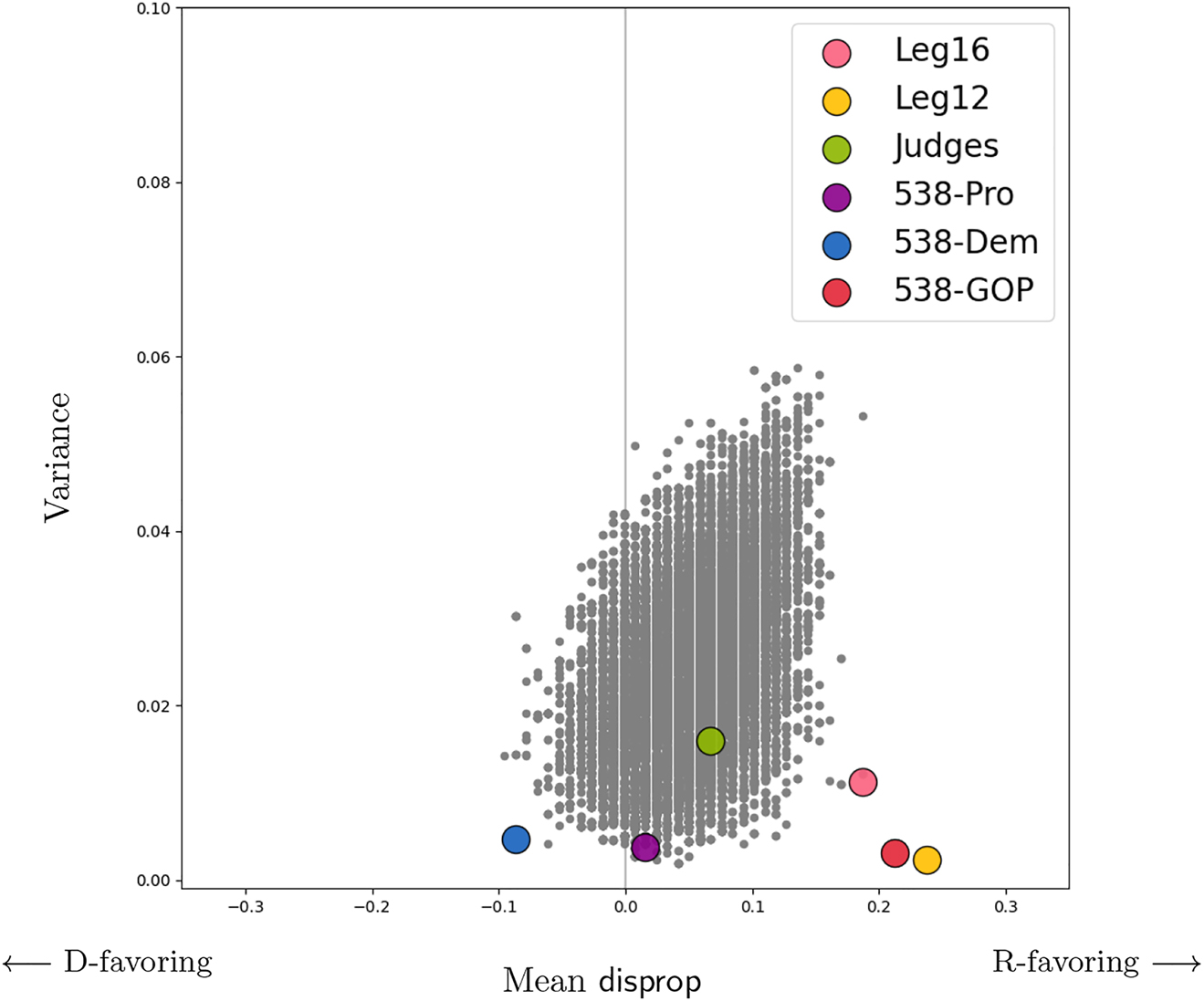
Statistics on disproportionality from North Carolina, with a party-neutral ensemble of 100,000 alternative plans plotted in gray. Handmade plans are marked with colored dots. Note that both legislative plans have high disproportionality, while the judges’ plan is much closer to a typical map in the ensemble. The 538 proportional plan succeeds at being very proportional with low variance, even though it was made using a different vote index. (This figure is repeated in Figure 5 below, alongside corresponding plots for the five other states studied here.)

Definition 2.

(Near proportionality). Given a threshold t > 0, a plan-election pair ( D , E ) is near-proportional if | d i s p r o p ( D , E ) |   < t .

This definition will help us study the FTV Test, which employed a threshold for Congressional plans of whichever is greater, one seat or 7%. That is, the language of the bill specified t = max (0.07, 1/k), where k is the number of seats. A proposed districting plan would be flagged as “materially favoring” a political party if its disproportionality exceeds t for at least two out of four recent Presidential and Senate elections. In other words, a plan needs to pass for at least three out of these four contests to pass the test overall. For example, if North Carolina’s enacted plan had been assessed in 2018 as part of the litigation that year, its pass rate in the previous two Senate and two Presidential races would be zero out of four, since the pro-Republican disproportionality is over 23% in all four elections, while the allowed threshold would be only 7.7% (one seat out of 13). The Judges’ plan reduces the disproportionality in every one of these four elections, but nevertheless also misses the mark all four times. This may not be surprising in light of the fact that the Judges did not have a mandate to design for proportionality, but instead to largely disregard partisanship. The ensemble comparison in Figure 1 gives us evidence that they succeeded.

In this paper we focus on assessing the soundness of the FTV Test, granting its choice of elections E 1 , … , E 4 and threshold t and considering possible standards to set the target for representation. We attempt to show that it is not too stringent and not too loose, applying a kind of Goldilocks principle.^[11] For us, the evidence that supports a positive Goldilocks conclusion is that at least 10% of a blind ensemble passes and at least 10% of a blind ensemble fails in every state but Massachusetts—and the test has an out that would work well in that hard case. Furthermore, the FTV Test and the use of a neutral ensemble of computer plans correctly handles the plans that came to us with a ground-truth label as gerrymandered, party-blind, or proportionality-seeking. It would be interesting to also consider how the choice of elections and thresholds interacts with the standard to make a sound test, but we leave further considerations in this direction to future work.^[12]

3 Validating Proportionality on Past Elections

Two questions are immediately posed by this discussion: first, how easy is it to design a near-proportional plan, even with perfect knowledge of the set of elections to be used in the test? And second, is past proportionality likely to predict future proportionality?

3.1 How Attainable is Near-Proportionality?

Figure 2 shows 100,000 population-balanced plans in each of six states, broken down by their success rate for near-proportionality in the four indicated elections.

Figure 2:

Breakdown of 100,000 districting plans on each of NC, PA, WI, MA, MD, and TX, scored by near-proportionality using the most recent two presidential and Senate races with t = max (0.07, 1/k), as in the FTV test. Each slice of the pie shows how many plans had a near proportionality score of X/4, with X ranging from 0 (red) to 4 (green), counter-clockwise around the circle. For each state, the blue and green sectors show the share of plans that would pass the test with three or four successes, respectively. More than a quarter of neutrally-drawn plans pass the test in North Carolina, Maryland, Texas, and Wisconsin; in Maryland, it’s well over half. Thousands pass in Pennsylvania, while none at all do so in Massachusetts.

In the states from our dataset, we can see appreciable differences in whether the central tendencies of PSMD support the selection of plans with near-proportional historical outcomes. It is fairly common (25–30% frequency) for our process to generate a near-proportional plan by chance in North Carolina and Texas, while enforcing only contiguity, population balance, and a preference for compactness. In Maryland and Wisconsin, it is even more frequent, occurring over 40% of the time in our sample. The Pennsylvania sample gives over 13,000 examples of compliant plans, i.e. more than one in eight plans that were generated passes the test. (Recall that only a single compliant plan is ultimately needed, with no badge of typicality required in the test.) Finally, in Massachusetts, a proportional plan simply never occurred in our sample.^[13]

Accordingly, ensemble evidence could clearly be used to protect an FTV-failing plan in Massachusetts from invalidation. Pennsylvania might attempt to rebut the presumption of a gerrymander, arguing that proportionality is difficult to secure. But on this reading of the bill’s intent, that attempt would fail and the other four states would have still more difficulty defending failing plans.

3.2 How Predictive is past Proportionality?

Given a plan that is shown to materially favor one party with respect to recent electoral data under a proportionality standard, is that property likely to persist into the future? Conversely, given a plan that secures proportional outcomes with respect to several past elections, how confident can we be that it will continue to do so? An empirical investigation of this question, starting again with North Carolina, is shown in Figures 3 and 4.^[14]

Figure 3:

A simple visualization of the predictive power of near-proportionality. Here, the training score is the number of near-proportional elections at t = 0.07 from an earlier set of contests. The test score shows the number of near-proportional elections with the same threshold for a later set of elections. In North Carolina, the proportionality performance on the later elections improves steadily as the earlier performance is increased. However, Massachusetts is different, as usual. The 2012–2014 period includes some election geography that makes it possible to achieve proportionality, so some maps earn a good training score. However, the 2016 and 2018 elections revert to form for the state, affording no instances of near-proportionality.

Figure 4:

Near-proportionality predictions, continued. All four of these states show an overall tendency for near-proportionality (t = 0.07) on earlier elections to secure improved proportionality on later elections. With a minor exception in Wisconsin, where plans with a training score of 0–1 slightly outperform those that score 2–3, higher training scores always secure higher average test scores.

In these plots, the top histogram shows the breakdown of the ensemble by training score, which is the number of near-proportional outcomes from the earlier elections. Below that are histograms showing the test scores (near-proportionality in later elections) for the subset of plans with each training score, in turn. (The language of “training” and “testing” is borrowed from machine learning, where one collection of data is used to fit a model and a second collection of data is used to test the success of the model at making a prediction or classification.)

For instance, the North Carolina ensemble has 36,711 plans with a training score of zero, shown in the red bar. Below that, the red histogram breaks those plans down by test score, showing that the most common test score is also zero, while the gray line marks their average test score at 0.59. There are 39 plans with a training score of 4, barely visible in the top histogram, and expanded in green below (average test score 3.72). Texas and Wisconsin had more training score values achieved in the ensemble than the other states, so the training scores are grouped in pairs.

The results are quite encouraging. In several states—North Carolina, Maryland, and Wisconsin—there is a pronounced trend for plans that are more often near-proportional in an earlier electoral window to stay so in a subsequent window. In Texas and Pennsylvania, there is not much variation in the test score, but the small differences incline the right way. Massachusetts, as usual, bucks the trend due to the uniform partisan geography in the later set of elections.

4 Finding Proportional Alternatives

In this section we present summary data showing that alternative plans can succeed from the point of view of average performance on the largest dataset available, as a complementary view to the serial performance considered above. We choose to average em scores rather than averaging the elections into a blended index. Election averaging, especially for a range of contests up and down the ballot, is fraught with issues of proper weighting given variable turnout, and can obscure consistent patterns that are important for understanding likely outcomes (see footnote 14 above).

When we do compute a mean disproportionality, the variance is also informative. If the state dataset includes elections that are variable in their party lean, then the mean and the variance of disprop combine to give a good view of a plan’s properties. Low-variance plans with disprop ≈ 0 across a diverse set of elections would be especially strong choices under a norm of proportionality. By contrast, the most egregious—and most successful—gerrymanders would have high-magnitude disprop and low variance.

In Figure 5, we present the data corresponding to North Carolina’s Figure 1 for other states under discussion. As in that figure, we include the Wasserman/538 Proportional, Democratic, and Republican plans. Notably, the 538 project used a different method to measure proportionality, using an election index based on averaging Presidential contests to designate a target seat split; this is then paired with Congressional voting history to gauge the lean of the seats.^[15] Thus, if the 538 proportionally partisan (“538-Pro”) map succeeds in FTV Test terms, it is a good sign that the FTV standard is robust to different ways of aiming at proportionality.

Figure 5:

The gray scatterplots show the mean and variance of disprop for each state’s ensemble of 100,000 plans. (The MA dataset looks smaller because many of the points coincide.) The colored dots show the corresponding data for plans made by people, including legislators, courts, and journalists. Besides legislative proposals and the 538 plans, these include a plan made by a bipartisan panel of retired judges in NC; a plan proposed by the Governor and a remedial plan ultimately adopted by the court in PA; and a limited modification of the legislative plan in TX that was drawn by a court (in the name of VRA compliance). Colored dots are vertically jittered for visibility. NC plot is repeated from Figure 1.

In Massachusetts, the enacted plan—which performs the same as 538-Dem—is typical of the ensemble. Maryland’s enacted plan is fairly D-favoring, with moderately low variance. By contrast, the benchmark plan from the previous cycle (though it would have become malapportioned in the intervening years) behaves similarly to the 538 Proportional map. In Pennsylvania, the 538 team used the same plan as both a Democratic and Proportional map. It is indeed fairly proportional, with disprop ≈ 0 and low variance. The 2011 enacted plan, the legislators’ proposed replacement plan from 2018, and the 538 Republican gerrymander are all strongly R-favoring, somewhat mitigated by moderate variance. The Texas 538 Proportional plan once again lives up to its name. The court’s VRA remedial plan displays a consistent Republican skew, with low variance, but the 538 Republican plan goes further. And Wisconsin follows the trend that a plan aimed at proportionality can succeed.

We can make a few other observations from the scatterplots. For instance, the Massachusetts scatterplot shows considerably higher variance than in the other states because it includes not only President and Senate races but also others such as Governor’s races, which can incline quite Republican in an otherwise Democratic-leaning state. The larger states (PA, TX) have more consistent statewide election shares, which contributes to lower variance in disproportionality.^[16]

5 Conclusions

The 50 United States are often called “laboratories of democracy,” and they are constitutionally entitled to construct state-specific legal frameworks for the “times, places, and manner” of elections, within the bounds of federal law. The manner includes a choice of systems (such as plurality elections in single-member districts, or PSMD) and a choice of norms for redistricting. For Congress, 45 of 50 states conducted PSMD elections in 2022.^[17] In this paper, we explore whether it might be compatible with PSMD for states to adopt proportionality as a goal for Congressional districting. We find evidence that the ease of securing a series of proportional outcomes varies by state, but that even party-blind redistricting can readily produce many examples in most states that we study—which includes all of the major legal hotspots from the previous Census cycle.

Our empirical work clarifies how to perform the simple “FTV Test” for extreme partisan gerrymanders that was set down in the draft legislation of the Freedom to Vote Act, and we confirm that the test is neither vacuous nor overly stringent. Applied with a proportionality target, the test requires that at least three out of four designated elections produce near-proportional outcomes; if not, then a reason for deviation must be provided to a court. We consider five states that were widely regarded as partisan gerrymanders and challenged in court, and one more (Massachusetts) that was not but that has a notable political geography. The results are summarized in Tables 2 and 3.^[18]

In Massachusetts, the legislature’s plan scores 0 out of 4 with all deviations in a Democratic direction, but in fact every one of our 100,000 blind plans scores 0 out of four in the same way, indicating that this disproportionality is explained (and likely forced) by political geography. This provides ample evidence to rebut the presumption of gerrymandering, and it fits with earlier research findings in (Duchin et al. 2019). The case of Massachusetts illustrates the utility of setting up the FTV test as a rebuttable presumption of gerrymandering, so as to avoid requiring what is potentially impossible. In the other five states, the 538 Proportional plan and at least 1/10 of a neutral districting ensemble pass the test. As noted above, the randomized algorithms employed here explore the central tendencies of the PSMD system, and it is common for a mapmaker with a goal to produce plans that surpass the extremes of a neutral ensemble. Together, the 538 and ensemble evidence should give a court ample grounds to deny an attempted rebuttal in these five states.

Proportionality is a straightforward and intuitive normative standard, and in most states studied here, it is achievable in a single-member/plurality district system without extreme partisan tuning—in every state but Massachusetts, a substantial share of maps from a partisan-blind process pass the test. Taken together, our findings provide ample evidence that the FTV Test for redistricting is sound when used with a proportionality target (and a safety valve of rebuttability), in that it is both manageable and reasonably comports with the “ground truth” determinations from courts that identified certain plans as impermissible partisan gerrymanders. This should provide encouraging empirical support for policymakers to reintroduce a similar test at the federal level, or to specify a proportionality target at the state level.

Though proportionality is not to be automatically expected from plurality in single-member districts, even absent a gerrymandering agenda, the findings here should raise our confidence that in many cases proportionality can nonetheless be pursued—and achieved.

References

Benadè, G., A. Procaccia, and J. T. Foltz. You Can Have Your Cake and Redistrict it Too. Preprint. Also available at https://www.gerdusbenade.com/files/21_gt.pdf.Suche in Google Scholar
Bycoffe, A., E. Koeze, D. Wasserman, and J. Wolfe. The Atlas of Redistricting. https://projects.fivethirtyeight.com/redistricting-maps/ (accessed January 25, 2018).Suche in Google Scholar
Campisi, M., T. Ratliff, S. Somersille, and E. Veomett. “Geography and Election Outcome Metric: An Introduction.” Election Law Journal 21 (3): 2022–219.10.1089/elj.2021.0054Suche in Google Scholar
Cannon, S., A. Goldbloom-Helzner, V. Gupta, J. N. Matthews, and B. Suwal. 2022. “Voting Rights, Markov Chains, and Optimization by Short Bursts.” Methodology and Computing in Applied Probability. to appear.10.1007/s11009-023-09994-1Suche in Google Scholar
Cover, B. P. 2018. “Quantifying Partisan Gerrymandering: An Evaluation of the Efficiency Gap Proposal.” Stanford Law Review 70: 1131.Suche in Google Scholar
DeFord, D., N. Dhamankar, M. Duchin, V. Gupta, M. McPike, G. Schoenbach, and K.-W. Sim. 2022. “Implementing Partisan Symmetry: Problems and Paradoxes.” Political Analysis. to appear, https://doi.org/10.1017/pan.2021.49.Suche in Google Scholar
DeFord, D., M. Duchin, and J. Solomon. 2021. “Recombination: A Family of Markov Chains for Redistricting.” Harvard Data Science Review 3 (1), https://doi.org/10.1162/99608f92.eb30390f.Suche in Google Scholar
DeFord, D., M. Duchin, and J. Solomon. 2020. “A Computational Approach to Measuring Vote Elasticity and Competitiveness.” Statistics and Public Policy 7 (1): 69–86, https://doi.org/10.1080/2330443x.2020.1777915.Suche in Google Scholar
DeFord, D., N. Eubank, and J. Rodden. 2021. “Partisan Dislocation: A Precinct-Level Measure of Representation and Gerrymandering.” Political Analysis 30 (3): 403–25, https://doi.org/10.1017/pan.2021.13.Suche in Google Scholar
Duchin, M., and M. Bernstein. 2017. “A Formula Goes to Court: Partisan Gerrymandering and the Efficiency Gap.” Notices of the American Mathematical Society 64 (9): 1020–4, https://doi.org/10.1090/noti1573.Suche in Google Scholar
Duchin, M., T. Gladkova, E. Henninger-Voss, B. Klingensmith, H. Newman, and H. Wheelen. 2019. “Locating the Representational Baseline: Republicans in Massachusetts.” Election Law Journal 18 (4): 388–401, https://doi.org/10.1089/elj.2018.0537.Suche in Google Scholar
Eguia, Jon X. 2022. “A Measure of Partisan Advantage in Redistricting.” Election Law Journal 21 (1): 84–103.10.1089/elj.2020.0691Suche in Google Scholar
Katz, J. N., G. King, and E. Rosenblatt. 2020. “Theoretical Foundations and Empirical Evaluations of Partisan Fairness in District-Based Democracies.” American Political Science Review 114 (1): 164–78, https://doi.org/10.1017/s000305541900056x.Suche in Google Scholar
Landau, Z., and F. Su. 2014. “Fair Division and Redistricting.” In The Mathematics of Decisions, Elections, and Games, 17–36. Providence, Rhode Island: American Mathematical Society.10.1090/conm/624/12472Suche in Google Scholar
MGGG Redistricting Lab. GerryChain Python Package. GitHub Repository. Also available at https://github.com/mggg/gerrychain.Suche in Google Scholar
MGGG Redistricting Lab. Paper Replication Materials. Also available at GitHub Repository. https://github.com/gabeschoenbach/Proportionality-Paper.Suche in Google Scholar
McGhee, E. 2017. “Measuring Efficiency in Redistricting.” Election Law Journal 16 (4), https://doi.org/10.1089/elj.2017.0453.Suche in Google Scholar
Rodden, J., and T. Weighill. 2022. “Political Geography and Representation: A Case Study of Districting in Pennsylvania.” In Chapter 5 in Political Geometry, edited by M. Duchin, and O. Walch. Birkhauser.10.1007/978-3-319-69161-9_5Suche in Google Scholar
S.2747 – Freedom to Vote Act. Also available at https://www.congress.gov/bill/117th-congress/senate-bill/2747/text.Suche in Google Scholar
Stephanopoulos, N., and E. McGhee. 2015. “Partisan Gerrymandering and the Efficiency Gap.” University of Chicago Law Review 82: 831–900.Suche in Google Scholar
Veomett, E. 2018. “Efficiency Gap, Voter Turnout, and the Efficiency Principle.” Election Law Journal 17 (4): 249–63, https://doi.org/10.1089/elj.2018.0488.Suche in Google Scholar
Warrington, G. S. 2018. “Quantifying Gerrymandering Using the Vote Distribution.” Election Law Journal 17 (1): 39–57, https://doi.org/10.1089/elj.2017.0447.Suche in Google Scholar
© 2023 the author(s), published by De Gruyter, Berlin/Boston
This work is licensed under the Creative Commons Attribution 4.0 International License.