Regional Environment Risk Assessment Over Space and Time: A Case of China
-
Xiangsheng Dou
 und
Fizza Ishaq
und
Fizza Ishaq

Abstract
Faced with increasingly serious environmental risks, it is necessary to conduct a comprehensive evaluation of the regional environment to provide a solid foundation for environmental policies and actions in the future. This article builds a composite environment risk index that considers spatiotemporal factors and uses annual socio-economic and environmental data of China’s 31 provincial administrative regions from 2004 to 2019 to quantitatively analyze environmental risks. Furthermore, the article employs a panel data model to empirically test the key factors that lead to environmental risks. Moreover, this article employs SVAR models to analyze the dynamics of regional environmental systems in China. The study finds that, at least at this stage, the environmental risks in provincial regions in China are still relatively high, and the key factors of the risks are economic growth, urbanization development, secondary industry growth, and green policy. Therefore, China must adopt more stringent environmental protection policies and actions in the future.
1 Introduction
To implement the Paris Agreement reached by the 193 member states of the United Nations in 2015 and achieve the Sustainable Development Goals (SDGs) by 2030, China has been actively taking comprehensive environmental protection actions to improve the environment at national and regional levels (United Nations, 2015a,b). However, due to differences in environmental resources and development conditions, different ecological and environmental situations may occur even if each region practices stricter environmental protection. This requires a scientific assessment of environmental risks. The spatial–temporal factor analysis of regional environment status can help every region recognize the existing problem, so as to further implement corresponding policies and measures toward the goal of the SDGs (Liu et al., 2021; United Nations, 2021).
The environmental quality of a region is determined by many factors, such as natural resources (especially water resources), natural disasters, waste discharge, and pollution treatment (Afridi et al., 2021; Bryan et al., 2018; Xu et al., 2020). In a certain period of time, if they change significantly or drastically, it indicates that the environment is at greater risk. In order to extract effective information from multi-dimensional environment indicators, it is necessary to construct a composite environment risk index to quantify environmental risks.
However, the construction of a composite environmental risk index faces two thorny issues. The first is that the indicators have different units and quantity levels, which can lead to heterogeneity and incompatibility of the indicators. This requires standardizing the raw data of the indicators through the scientific method. Another is the determination of the weight of each indicator in the total composite index, as it needs to consider the dual effects of time and space.
At present, multi-level and multi-indicator evaluation methods have been widely used, and some composite indexes, such as the Bertelsmann Index (Lafortune et al., 2018; Miola & Schiltz, 2019; Sachs et al., 2018, 2021) and the Distance Measure Index (OECD, 2017), have constructed. The SDG Index used for sustainability evaluation is another famous composite index. It was constructed through multi-dimensional indicators, which have achieved good results in actual evaluation (Halkos & Argyropoulou, 2022).
However, due to the need to address the issue of the different units of indicator data and the objective determination of weights for each indicator in the application of multi-indicator synthesis methods, further improvement and refinement is necessary. Especially, the existing methods do not solve the heterogeneity of the indicators of variables, because they only perform general non-dimensionalization (such as range standardization and non-dimensionalization) of the variable’s indicators (Li, 2021; Liu et al., 2019; Streimikiene et al., 2021). Moreover, when synthesizing different index of variables, the weight of each index needs to be determined first, but the usual method (e.g., simple average method, subjective scoring method, and fuzzy decision method) has greater subjectivity, which affects the reliability of the measurement (Dhiman & Deb, 2020; Ervural et al., 2018; Palczewski & Sałabun, 2019).
In order to improve the reliability of the measurement, this article makes an improvement from three aspects. First, the relative distance between individuals and their mean is used to define the risks. The mean here contains the dual information of a specific indicator at different times and different spaces. This method can not only realize the dimensionlessness of the index of the variable but also enhance the comparability of the results over time and space.
Second, the article unitizes the risk variables defined above to ensure that the calculated values of each relative risk index are within the range of 0 and 1. This method can not only realize the homogeneity, comparability, and synthesizing of data but also reduce the problem of possible divergence and instability (Dou, 2022).
Finally, the article uses the unitized index data to calculate the weights. Because of the homogeneity of the unitized data, it may realize the scientific determination of the weights in the calculation of the composite index when they are used to determine the weight. It solves the uncertainty of weight determination in traditional multi-standard decision analysis such as simple average method, subjective scoring method, and fuzzy decision method.
The research shows that the composite risk index proposed here is suitable for the evaluation of complex system objects such as natural ecological and environmental systems. Moreover, it can also be applied to more complex cases and more broad fields such as society, economy, finance, management, technology, and so on.
This article attempts to addresses three problems using our own method and model. First of all, what is the actual situation of the environment (risks) in each region. Second, what is the dynamic evolution process and trend of the environment (risks) in each region over time. Third, the article empirically analyses the key factors that lead to the environmental risks in various regions.
The study finds that the environment quality of each province-level region is unstable during the selected sample period, and most of the regions are in a risk or high-risk state in recent years. The empirical results indicate that the key factors leading to environmental risks are economic growth, urbanization development, secondary industry growth, and green policies (e.g., environmental governance, environmental protection investment, energy safety, technologies and innovations, environmental education, and environmental sensitivity). Generally, economic growth, secondary industry growth, and green policies are conducive to reducing environmental risks, while urbanization will exacerbate environmental risks.
The remainder of the article is structured as follows. The second section elaborates on environmental risk measurement and evaluation. The third section is an empirical analysis of the determinants of regional environmental risks. Section 4 is a dynamic test of the regional environment system. In Section 5, we discuss the results. The last is the conclusion.
2 Measurement and Evaluation of Regional Environment Risks
2.1 Method and Model
We first consider the case of a general two-level indicator system here. We use
Our goal is to perform a weighted average of the variable values (
where
Similarly, the calculated first-level comprehensive indicators (
where
In order to achieve comparability over time and space, different individuals and times of the same index (including primary and secondary indicators) use the same weight. That is:
The above is a general solution idea. In order to measure the environmental risk, let us redefine the value of the variable X. For the sake of simplicity, we here use the absolute value of the relative deviation to measure the risk, and it is calculated as follows:
where
However, due to the different orders of magnitude of different indicators including the first and second levels, the difference in the risk values is often large and lacks comparability, which brings difficulties to the determination of the weights. It has puzzled academia in the construction of the composite index of multidimensional indicators for a long time.
Traditional methods of weight determination are often subjective, which reduces the credibility of research results. In order to solve this problem, we will unitize (process through logistic function conversion) the risk value (
where
For the variable value
where
The weight of the corresponding second-level index
where
The unit risk composite index
Similarly, we can calculate the weight
where
We can calculate the final unit risk index (UERI) of each individual i in different periods from formulas (9) and (11) as follows:
The unit risk index (UERI) is de-unitized and multiplied by 100 to obtain the composite risk index (ERI) for different periods as follows:
2.2 Indicator and Data
Generally, the broad sense of space should include three aspects: geographical space, international space, and China’s regional space (Streimikiene et al., 2020, 2021; Streimikiene & Kyriakopoulos, 2023). However, this article focuses on the study of China/s provincial administrative region (space). Due to the vast territory of China and the distinct characteristics of each region, the use of provincial-level regional sample data in China has good display performance. As for the time dimension, theoretically, the longer the time, the better the display. However, in practice, too long a time span can lead to data incompatibility, as early China did not pay attention to environmental issues until the beginning of this century when they gradually became more important. In addition, there is also an issue of early data loss. Therefore, the sample period selected in this article is from 2004 to 2019.
Considering the availability of data, the conciseness of research, and the comparability of results, this article selects indicators from four dimensions such as water resources, natural disasters, waste discharge, and environmental governance investment, as their changes can directly lead to fluctuations and risks in the environmental system.
Furthermore, the indicator of the water resources has three sub-indicators of surface water, groundwater, and other water resources (unit: 100 million cubic meters). The indicators of natural disaster have four sub-indicators, including flood, drought, wind, and hail disaster and freezing disaster (unit: thousand hectares). The indicators of waste discharge has three sub-indicators of wastewater, waste gas, and garbage (unit: 10,000 tons). The indicators of environmental governance investment include six sub-indicators such as waste water, waste gas, solid waste, noise, other governance, and forestry project investment (unit: ten thousand yuan) (Dou, 2015, 2016; González-González et al., 2021; Noori et al., 2021; Shi & Moser, 2021).
This article uses annual data of 31 provincial administrative regions in China from 2004 to 2019. The raw data come from China’s National Bureau of Statistic (2021). In order to improve the reliability of the measurement results, we have performed statistical processing on individual missing or abnormal data.
2.3 Results and Evaluation
2.3.1 Descriptive Statistical Analysis
Figure 1 shows the descriptive statistics of the environment risks of 31 provincial administrative regions in China. Obviously, almost all the provincial regions show a skewed distribution. However, Shanxi, Liaoning, Jiangxi, Shandong, Hubei and Shaanxi show significant left-skewed distributions, while other regions show right-skewed distributions. This indicates that the environment risks in most areas are high.
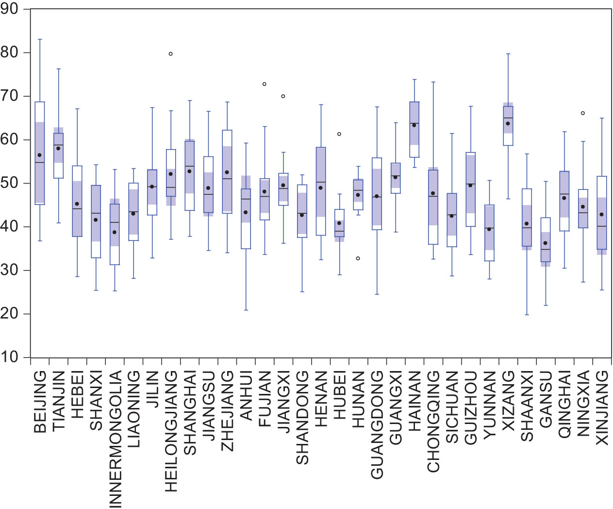
Box plot of the ecological risk index of each provincial region.
In terms of maximum value, Beijing has the highest maximum value, and Xizang is in second place. Moreover, the maximum value of Tianjin, Hainan, and Chongqing is significantly higher than other regions.
In terms of minimum value, Shaanxi and Anhui have the same and the lowest minimum, and Gansu has the second minimum. In addition, Shandong, Guangdong, Inner Mongolia, and Shaanxi have minimum values that are relatively close and slightly higher than Gansu.
As for the mean value, Xizang has the largest mean value, Hainan’s mean value is second and closer to Xizang, and Gansu’s mean value is the smallest. This result is closely related to the special natural and socio-economic conditions of each region.
2.3.2 Change in Environment Risks
The research indicates that, the environment of 31 provincial regions in mainland China shows an unstable state during the sample period. Moreover, most of the provincial-level regions have large fluctuations.
We find that, first of all, the time trend of environment changes in most areas is not significant, and it does not show significantly and relatively stable phase characteristics. Second, the environment in most regions shows divergent changes. Finally, although the environmental protection policies and measures of the national and various regions have become increasingly strict in recent years, the phenomenon of tail-lifting is prominent (Figure 2).
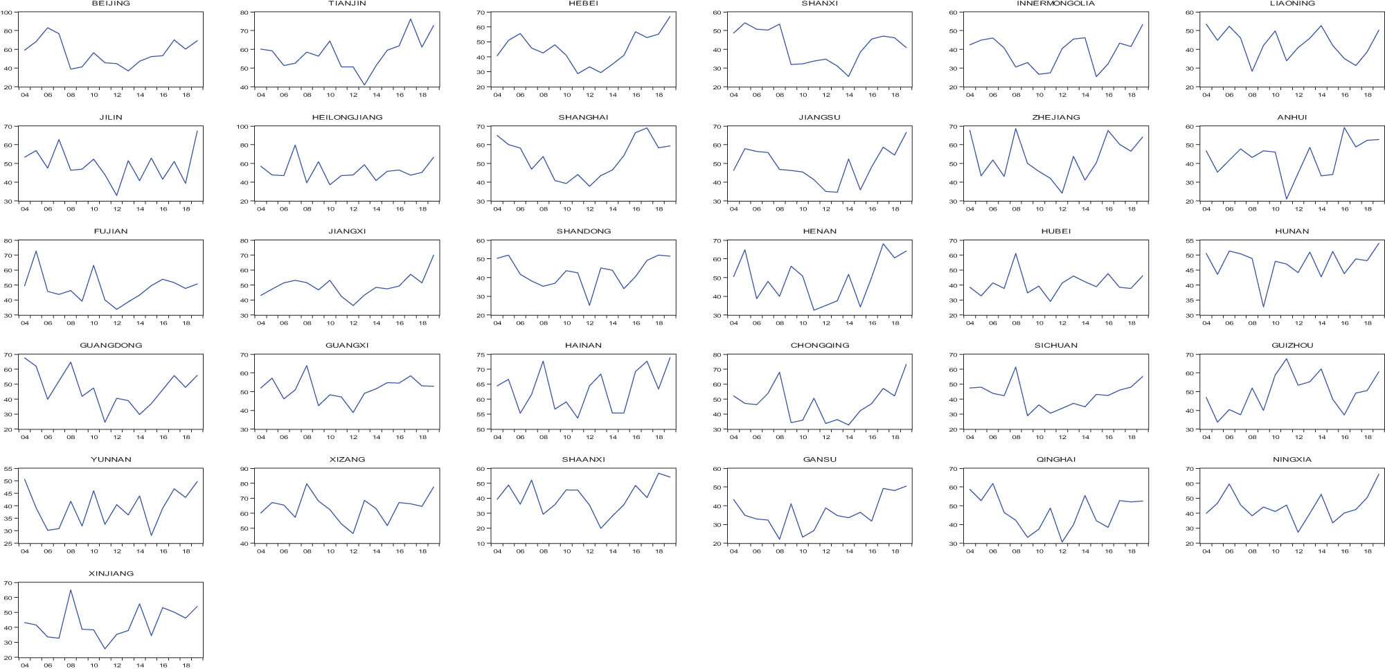
Changes in environmental risks in provincial regions.
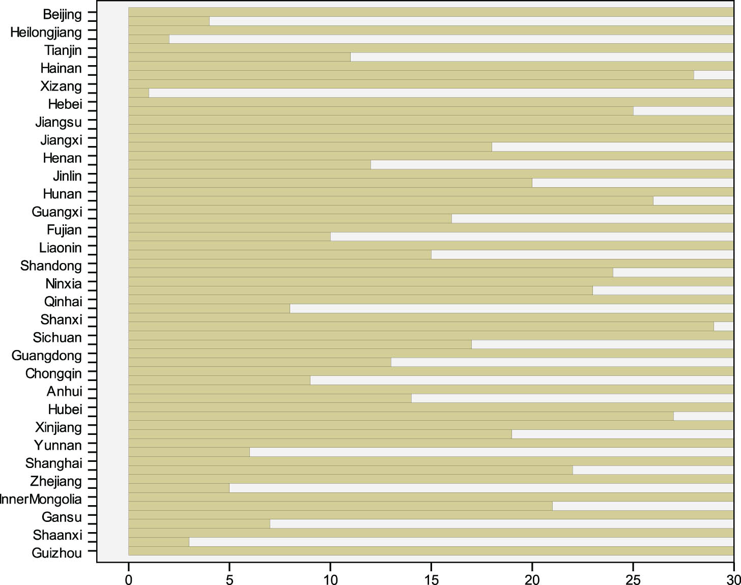
2.3.3 Analysis of Environmental Risk Dashboard Graph
For the sake of intuitive analysis, we divide the environmental risk index from 0 to 100 into five levels: (0, 20), (20, 40), (40, 60), (60, 80), and (80, 100). They represent no-risk, low-risk, risk, high-risk, and extreme risk, respectively. Correspondingly, we use dark green, light green, yellow, blue, and red squares to represent them, respectively. Then, we draw a Dashboard graph according to the various provincial regions in different years (Schmidt-Traub et al., 2017).
Figure 3 shows that most of the province-level regions in China have high environmental risks, and they have been in a risky or high-risk state in recent years. The environmental risks in Beijing are relatively high in the early stage, which has improved slightly after governance, but become serious in the later stage. This shows that the environmental pressure on Beijing, the capital of China, is increasing. Tianjin, Shanghai, and Zhejiang have similar situations to Beijing, but to a lesser degree.
![Figure 3
SDG Dashboards 2004–2019. Note: We divide the environment risk index from 0 to 100 into five levels: [0, 20], [20, 40], [40, 60), [60, 80], and [80, 100]. They respectively indicate no risk, low risk, risk, high risk, and extreme risk. Correspondingly, we use dark green (), light green (), yellow (), blue (), and red () squares to represent them, respectively.](/document/doi/10.1515/econ-2022-0049/asset/graphic/j_econ-2022-0049_fig_003.jpg)
SDG Dashboards 2004–2019. Note: We divide the environment risk index from 0 to 100 into five levels: [0, 20], [20, 40], [40, 60), [60, 80], and [80, 100]. They respectively indicate no risk, low risk, risk, high risk, and extreme risk. Correspondingly, we use dark green ( ), light green (
 ), yellow (
 ), blue (
 ), and red (
 ) squares to represent them, respectively.
Among the 31 provincial-level regions, Xizang has the most prominent environmental problems with 12 blue and 4 yellow in the sample period, which is significantly at risk and high risk. Followed by Hainan, there are 10 blue and 6 yellow in the sample period, which is also at risk and high risk. This may be closely related to the special conditions of the two provincial regions.
2.4 Regional Comparative Analysis
In order to better examine the particularities of each region, we used systematic cluster analysis to classify the environmental risks of China’s 31 provincial administrative regions (Figure 4). According to Figure 4 and our research purpose, we divide them into seven types.
The ice chart of hierarchical cluster analysis.
Among the seven types, Beijing (Type I), Heilongjiang (Type II), and Guizhou (Type VII) become a separate category, which shows that they are quite different from other regions, and have their own environment and socio-economic characteristics. Beijing, as the capital of China, despite its huge investment in environmental protection, the excessive accumulation of population and economic resources has led to greater risks to the environment. Heilongjiang is located in the northernmost part of China, and is one of the three northeastern provinces that are lagging behind in development at this stage. Although its ecological conditions are relatively good, its socio-economic conditions are relatively weak. Guizhou is one of the most underdeveloped regions in China and has a relatively special natural environment as well as a relatively backward social economy.
Type III includes three regions of Tianjin, Hainan, and Xizang. Tianjin is one of the most developed regions in China, but water resources are scarce and the natural environment is highly volatile. Hainan is an independent island with rich tropical biological resources, but the environmental and socio-economic conditions have changed significantly due to large-scale development in recent years. Xizang is an area with rich ecological resources but the most fragile natural ecosystem in China, so it is greatly affected by climate change. The high environmental risks of Hainan Province and Xizang Autonomous Region are inseparable from their own special environment and climatic conditions. Natural disasters occur frequently in Hainan Province, while the ecological environment of the Xizang Autonomous Region is fragile and natural disasters occur frequently. Therefore, the environment management in these special areas is difficult.
Shanghai and Zhejiang are Type V regions. They are all developed areas in China and geographically adjacent, but the area of jurisdiction is relatively small. Because of their excessive concentration of population and economic resources, they have similar ecological and environmental risks.
InnerMongolia, Gansu, and Shaanxi in Type VI are located in the northwestern region of China, and their environment has similarities. InnerMongolia is one of the most developed areas of animal husbandry in China, but the environment is at a relatively high risk due to pasture degradation and extreme climate change. Both Gansu and Shaanxi have a serious water shortage and drought problem, which has led to serious soil desertification and soil erosion. Therefore, their environmental risks are prominent.
Except for the above six types of regions, the rest of the regions belong to Type IV, which covers 20 provincial administrative regions. For example, Hebei, Shanxi, Liaoning, Jilin, Jiangsu, Anhui, Fujian, Jiangxi, Shandong, Henan, Hubei, Hunan, Guangdong, Guangxi, Chongqing, Sichuan, Yunnan, Qinghai, Ningxia, and Xinjiang. They can be geographically divided into the eastern coastal region (Fujian, Guangdong, Jiangsu, and Shandong), the northwest region (Qinghai, Ningxia, and Xinjiang), the southwest region (Guangxi, Sichuan, and Yunnan), and the central inland region (the rest). The environmental risks in these areas are either caused by the environmental governance lagging behind the socio-economic development or caused by the shortage of water resources and climate change or caused by the combination of the two.
3 Determinants of Regional Environmental Risks
3.1 Model and Data
The environmental risk of a region is determined by many factors. However, for China at this stage, the effects of several key socio-economic factors are important. The first is the impact of economic growth on the environment. On the one hand, economic growth has a negative impact on the environment; on the other hand, economic growth has increased the fiscal revenue of regional governments, and it will help the government to increase investment in environmental governance, which is conducive to the improvement of the environment (Li et al., 2021; Shi et al., 2020).
The growth of the secondary industry has both favorable and unfavorable effects. At this stage, as the secondary industry occupies a large proportion of GDP, its development can significantly promote economic growth. At the same time, since the secondary industry has the characteristics of high inputs, high energy consumption, high outputs, and high emissions, it has an adverse impact on the environment. The final result depends on the strength of the both (Chen et al., 2020; Zhang & Liu, 2021).
In recent years, China’s urbanization has developed rapidly, but the impact of urbanization on the environment is significant. First of all, the development of urbanization (especially the development of small cities) directly erodes the environmental resources such as land resources, forest resources, and water resources, and this impact is irreversible. Second, although urbanization has a resource agglomeration effect, the city itself needs to consume a lot of resources and produce a lot of waste, which has a significant adverse impact on the environment (Ahmed et al., 2020; Yao et al., 2021).
Green policies play an important role in improving the environment. China has not only adopted strict environmental protection policies but has also continuously increased its investment in environmental governance. In terms of industrial policies, the state has been investing large amounts of financial funds in recent years to transform traditional high-energy-consumption and high-pollution industries, and actively support the development of green and low-carbon industries. At present, the government has formulated and implemented a complete set of green policies, which has fundamentally improved the environment (Cao et al., 2021; Qin et al., 2021; Yang et al., 2021).
According to the above theoretical analysis and considering the reality of China’s economic development and environmental changes at this stage, this article selects the key factors of economic growth, secondary industry growth, urbanization development, and green policy for empirical analysis. The equation is set as follows:
where ERI stands for environment risk, ED stands for economic growth, GP stands for green policy, IR stands for secondary industry growth, UR stands for urbanization development, i represents cross-sectional individual, t means time, and ε is white noise series.
Because the socioeconomic development and the natural environment of the regions are different, the environmental risks of the regions in China are different. In order to clarify the real situation of the environment in various regions, this article takes 31 provincial administrative regions in mainland China as the research object, and the sample period is from 2004 to 2019. All data come from the yearbook of the National Bureau of Statistics (2021).
3.2 Baseline Model Estimation
Table 1 reports the estimation results of equation (14). It can be seen that economic growth (ED), urbanization development (UR), secondary industry growth (IR), and green policies (GP) have all a significant impact on the environment. The empirical results show that the faster the economic growth of a region, the smaller the environmental risk in the region. This is because the government has attached great importance to environmental protection in recent years, which has forced the government to increase financial investment in environmental governance as much as possible, while economic growth has laid the financial foundation for the government to increase financial investment. In addition, strict ecological and environmental protection policies have reduced the impact of social and economic development on the environment.
The estimation result of the equation (14)
| Variable | Coefficient | Std. Error | T-Statistic | Prob. |
|---|---|---|---|---|
| LnED | −0.0570 | 0.0273 | 2.0917 | 0.0370 |
| LnGP | −0.0721 | 0.0293 | 2.4591 | 0.0143 |
| LnIR | −0.4544 | 0.0681 | 6.6748 | 0.0000 |
| LnUR | 0.1986 | 0.0912 | 2.1789 | 0.0298 |
| C | 5.4115 | 0.3724 | 14.5300 | 0.0000 |
In theory, the development of the secondary industry can make an adverse impact on the environment. However, the empirical results here show that it is beneficial to reduce environmental risks (Table 1). One possible explanation is that the key secondary industries in all regions are concentrated in cities, and the government has implemented strict environmental protection policies for industrial enterprises with high energy consumption, high emissions, and high pollution, which has prompted enterprises to improve efficiency (Chen et al., 2020), thereby minimizing the adverse effects of the development of the secondary industry on the environment. Moreover, since the secondary industry accounts for a large proportion of GDP at this stage, the better the development of the secondary industry in a region, the faster the economic growth, which is conducive to improving the environment.
The implementation of the green policy is important to the improvement of the environment, as it helps to significantly reduce the environmental risks. The role of the green policy is that it not only increases the financial investment of the central government and the regional governments in the governance of the environment but also strictly restricts the economic behavior of economic agents that may deteriorate the environment. In recent years, the breadth and depth of the implementation of green policies in all regions has been continuously increasing, effectively reversing the continuous deterioration of the environment in the early stages of reform and opening up (Kahn et al., 2022).
The empirical results show that the development of urbanization will exacerbate the environmental risks. China’s urbanization is characterized by extensive and rapid progress. The first is that all regions have been making great efforts to promote urbanization, which not only encroaches on a large amount of land, forests, and other ecological resources, but also the excessive expansion of the city in the short term, resulting in a large population agglomeration and industrial development, has caused the growth of urban wastes to make great pressure on the environment. Second, the development of some small- and medium-sized cities lacks scientific planning and strict governance, resulting in a comprehensive and irreversible impact on the local environment.
3.3 Analysis of Individual Differences
Figure 5 reports the differences of the individuals. We can find that the environmental risks of provincial administrative regions in China are different. From the perspective of individual differences, the environmental risk level of Beijing, InnerMongolia, Yunnan, and Gansu is below 5.3. Nine areas, including Liaoning, Jilin, and Jilin, Shanghai, Anhui, Shandong, Hubei, Sichuan, Shaanxi, and Xinjiang, are between 5.3 and 5.4. Twelve areas, such as Hebei, Shanxi, Heilongjiang, Fujian, Hunan, Guangdong, Guangxi, Hainan, Chongqing, Guizhou, Qinghai and Ningxia, are between 5.4 and 5.5. Five areas, including Tianjin, Jiangsu, Zhejiang, Jiangxi, and Henan, are between 5.5 and 5.6. Only Xizang is above 5.6.
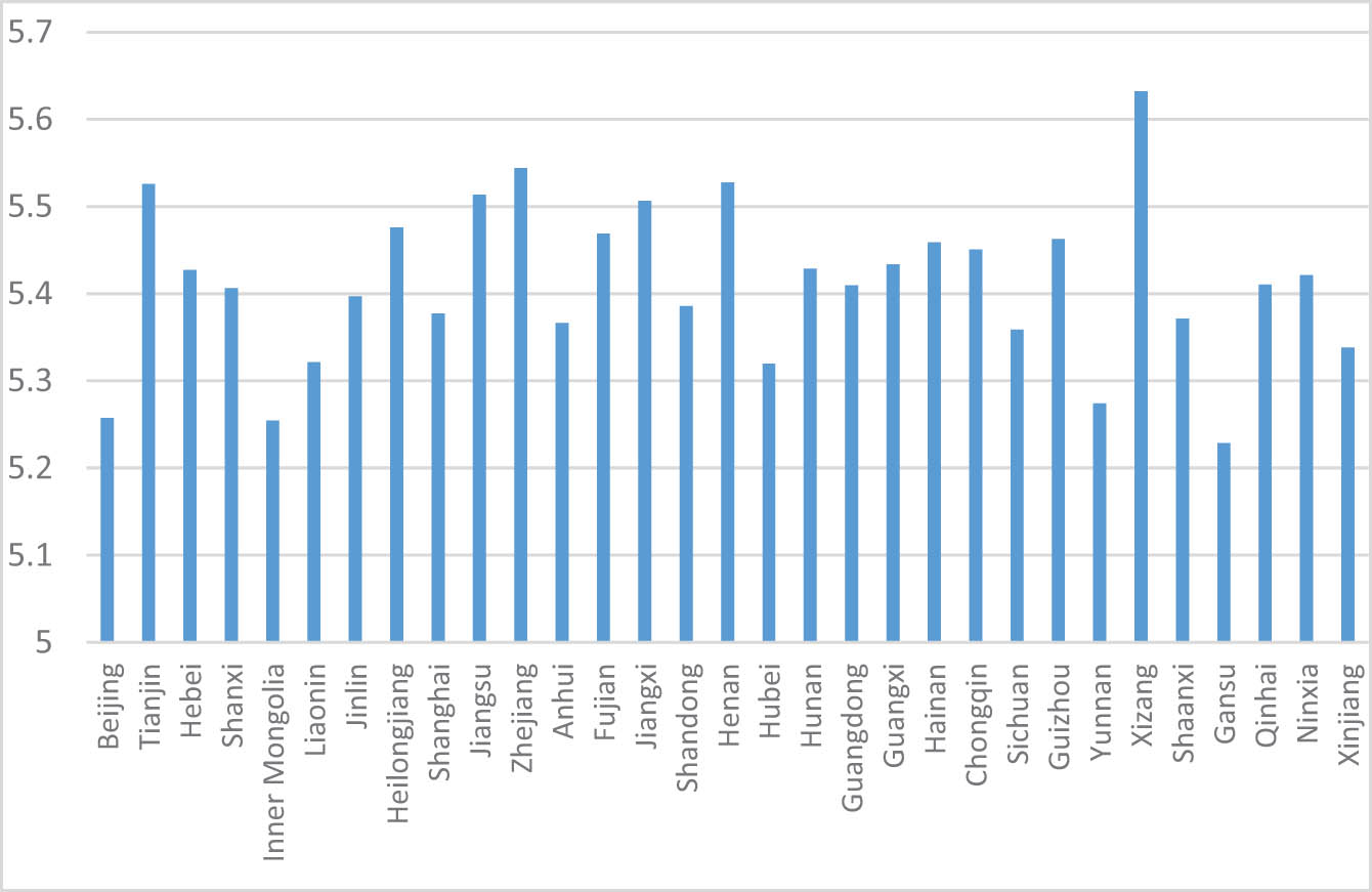
The differences of individuals.
The individual differences of different provincial administrative regions are caused by the differences in the endowment of environmental resources, the level of social and economic development, and the degree of environmental protection and governance in each region, and the environment of a region is jointly determined by these key factors. However, due to the large differences in these factors and conditions in different provincial administrative regions in China at this stage, the emergence of individual differences is inevitable. This shows that the environmental protection and governance of the regions in China must adopt corresponding policies in accordance with their own actual situation in the future.
3.4 Robustness Test
In order to test the reliability of the estimation results of the equation, we reduce the scope of the sample to re-estimate equation (14). Table 2 reports the estimation results. It shows that the influence of all explanatory variables is still statistically significant, the sign of each coefficient has not changed, and the value of the coefficient only has a small change compared with Table 1. This demonstrates that the estimation results of equation (14) are reliable.
The results of robustness test
| Variable | Coefficient | Std. Error | T-Statistic | Prob. |
|---|---|---|---|---|
| LnED | −0.0835 | 0.3730 | 3.0358 | 0.0025 |
| LnGP | −0.0945 | 0.0302 | 3.1339 | 0.0018 |
| LnIR | −0.4032 | 0.0696 | 5.7932 | 0.0000 |
| LnUR | 0.1829 | 0.0907 | 2.0163 | 0.0443 |
| C | 5.5632 | 0.3727 | 14.9268 | 0.0000 |
4 Dynamic Test of Regional Environment System
This study applies the SVAR model to investigate how several factors affect the dynamic changes of the ecological environment system. We specify the model as follows:
where B 0 represents the coefficient matrix of the current period, Γ0 represents the constant term, Γ i (i = 1, 2, …, p) represents the coefficient matrix of the lag period, y represents the variable matrix in the system and y = (ERI, ED, GP, IR, UR)′, u is white noise series, and t is the time (t = 1, 2, …, n).
The SVAR model can not only describe the current relationship between the variables in the system but also describe the structural relationship of each period compared with the VAR model. Therefore, it can better characterize the dynamic influence of the variables in the system.
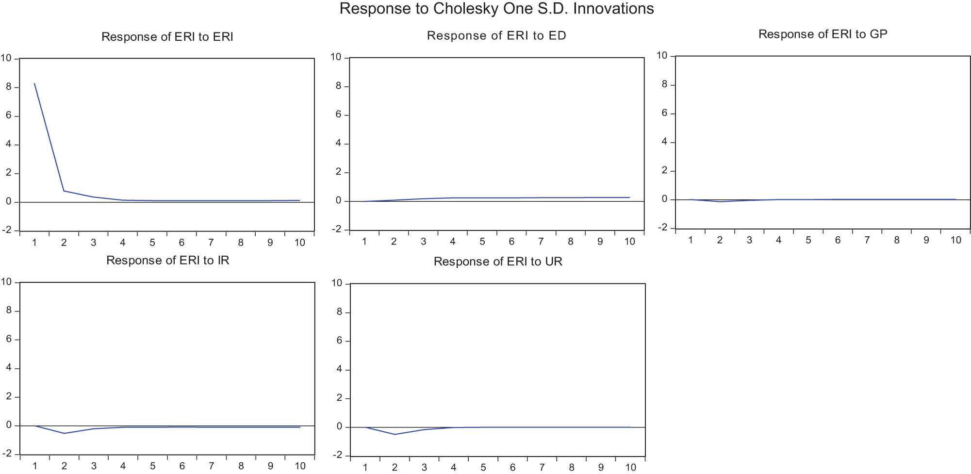
4.1 Dynamics of Type I Areas
Figure 6 reports the dynamics of ecosystems in Type I regions. The self-shock impact caused by changes in ecological risk (ERI) has the characteristics of significant convergence and periodic changes. It decreases sharply in the second period, rapidly in the third to sixth period, but stabilizes and converges to the mean value after the sixth period. This shows that although the ecological risk variable (ERI) has a certain degree of self-perturbation, it tends to be gradually stable over time.
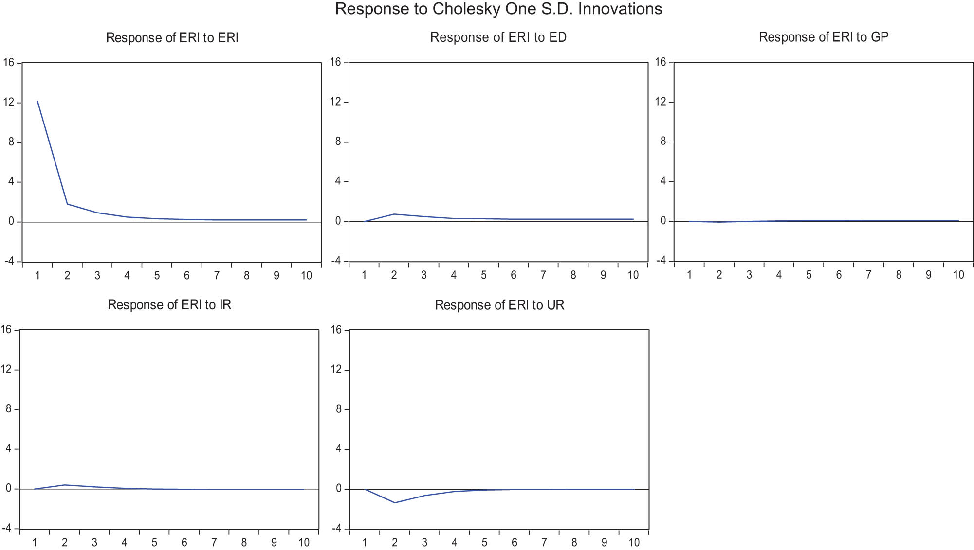
Impulsive response of ERI to other variables in type I.
The change in economic growth (ED) has a certain positive impact on the ecological environment (ERI), but the impact is relatively small. The disturbance caused by it is relatively large from the first period to the fifth period, but it is in a relatively stable state of change after the sixth period. However, the disturbance it causes does not converge to the mean.
The change in green policy (GP) has relatively little disruption to the ecosystem. From the first period to the fourth period, it has almost no effect. It produces a certain disturbance after the fifth period, but the impact is small (almost converges to the mean value) and shows a stable state.
The development of the secondary industry (IR) has a certain impact on the ecological environment (ERI) as a whole, and there is a phenomenon of alternating positive and negative impacts. It has a positive effect in periods 1–4, but little effect in periods 4–7. However, it has a negative effect after the 7th period, but this effect is small and shows a stable trend.
Urbanization development (UR) has a disturbing effect on the ecological environment (ERI). It leads to a significant negative change in the ecological environment (ERI) during the first to the fifth period, while the change caused by it is significantly smaller and shows a stable state from the fifth to the eighth period. However, it converges to its mean value after period 8 (Figure 6).
4.2 Dynamics of Type II Areas
In Type II areas, the self-shock effects caused by changes in ecological risk (ERI) are complex. During periods 1–2, the effect it caused drops sharply and goes from positive to negative. The negative volatility it causes becomes smaller after period 2, but it has a small positive volatility and converges to its mean in period 3. After period 6, it has another slight negative swing, but the swing is smaller (Figure 7).
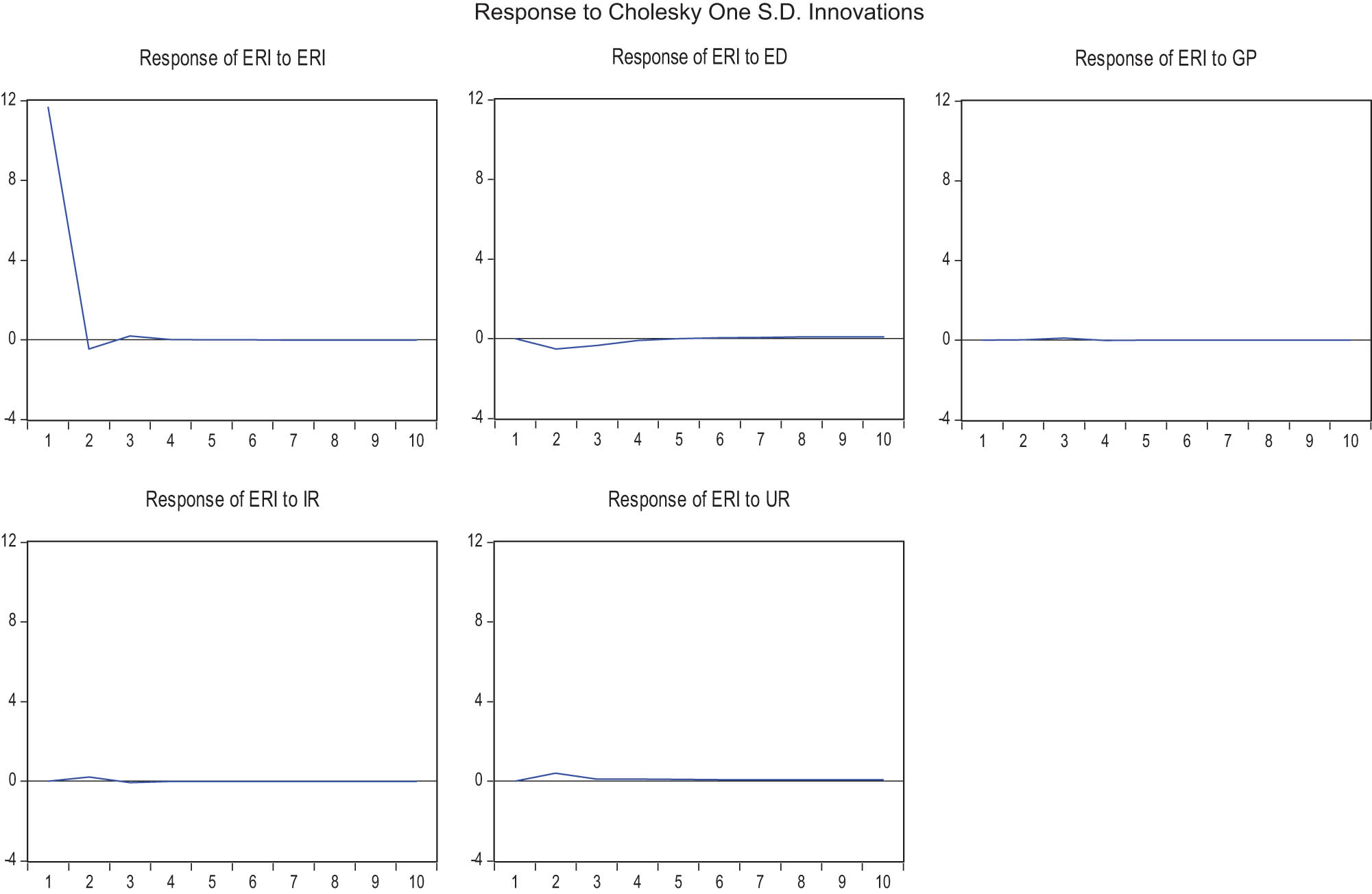
Impulsive response of ERI to other variables in type II.
The disturbing effects of changes in economic growth (ED) on the ecosystem (ERI) are complex. From the first period to the fourth period, it has a significant negative disturbance, and the disturbance effect gradually becomes larger from the first period to the second period, but becomes smaller from the third period. After the fourth period, its perturbation converges to the mean and continues until the seventh period. After period 7, it produces positive disturbances, but the fluctuations are small and relatively stable (Figure 7).
Figure 7 shows that change in green policy (GP) has less perturbation effect on the ecosystem (ERI). It converges to its mean value in all other periods except for a slight positive perturbation in periods 2–4. Therefore, green policies are conducive to improving the ecological environment.
For Type II regions, the disturbance of the secondary industry development (IR) on the ecological environment (ERI) is small. Except for a slight positive perturbation in periods 1–3, it converges to the mean in all other periods (Figure 7).
Urbanization development (UR) has always a positive disturbance effect on the ecological environment (ERI). In the first to third period, the positive change caused by it is significant. But after the third period, the change it caused is significantly smaller and shows a stable state (Figure 7).
4.3 Dynamics of Type III Areas
In Type III regions, the self-shock impacts of change in ecological risk (ERI) are complex. During periods 1–2, it results in a positive effect with a sharp decline. After period 2, its positive volatility gradually becomes smaller. It converges to its mean during periods 3–4. After period 4, it has a slight negative swing and has been trending steadily (Figure 8).
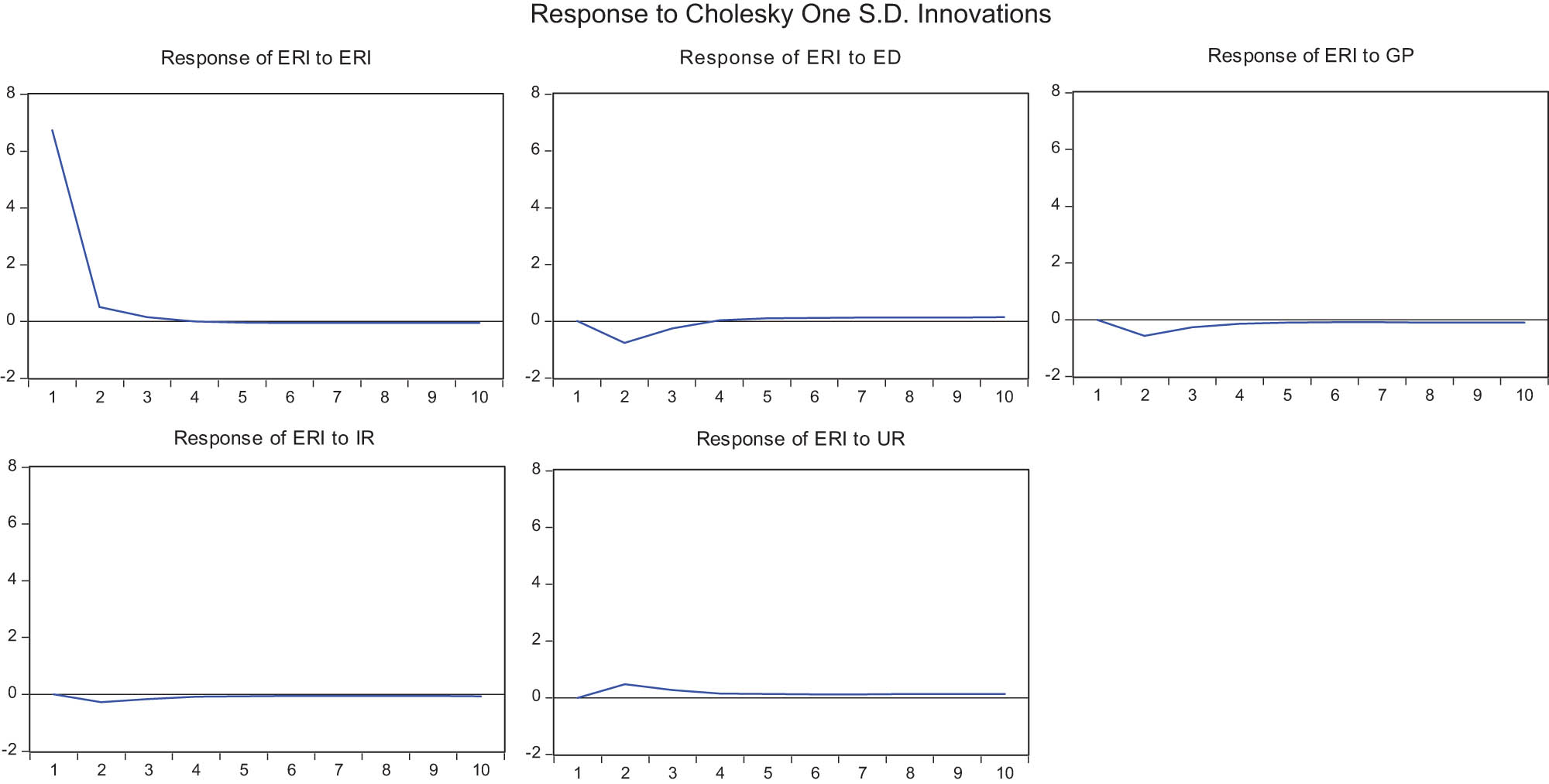
Impulsive response of ERI to other variables in type III.
The disturbing effects of change in economic growth (ED) on the ecosystem (ERI) are complex. It has a significant negative perturbation effect from the first period to the fourth period, and its perturbation effect gradually becomes larger during the first period to the second period, but it becomes smaller after the third period. After the fourth period, it produces a positive disturbance effect, and its disturbance effect becomes slightly larger and shows a relatively stable state from the fifth period (Figure 8).
The disturbances caused by changes in green policy (GP) to the ecosystem (ERI) have always shown negative changes. It produces a significant negative perturbation effect during the periods 1–4. However, its negative perturbation effect begins to become smaller and shows a relatively stable state after the fourth period (Figure 8).
Figure 8 shows that the development of the secondary industry (IR) has always a negative disturbing effect on the ecological environment system (ERI). The negative disturbance generated by it is relatively large from the first period to the fourth period, but then becomes smaller and shows a relatively stable state.
Urbanization development (UR) has always a positive disturbance effect on the ecological environment (ERI). However, the positive change caused by it is relatively significant during periods 1–4, but then becomes smaller and relatively stable (Figure 8).
4.4 Dynamics of Type IV Areas
Figure 9 reports the dynamics of the ecological environment (ERI) system in the Type IV areas. The self-shock impacts caused by the change in ecological risk (ERI) have the characteristics of stages. It shows a positive effect and declines sharply during periods 1–2. However, its positive volatility gradually becomes smaller from period 2 to period 4. Further, it converges to its mean during periods 4–6, but has a slight negative fluctuation and has been showing a stable trend after the sixth period (Figure 9).
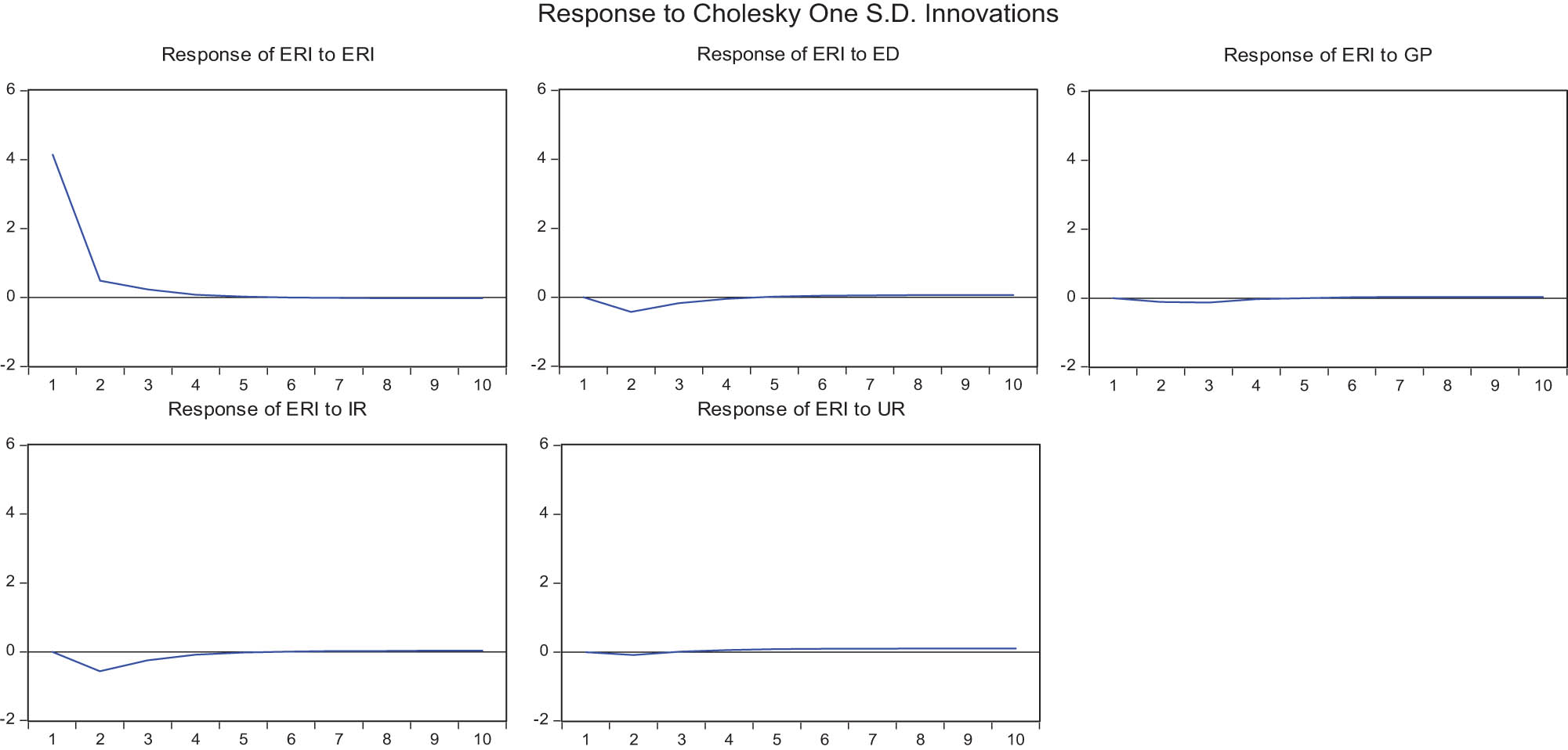
Impulsive response of ERI to other variables in type IV.
The disturbing effects of changes in economic growth (ED) on the ecosystem (ERI) are complex. it has a significant negative perturbation effect from the first to the fourth periods, and its perturbation effect gradually becomes larger during the first to the second period, but it becomes smaller from the third period. Furthermore, it converges to its mean during periods 4–6, and it produces relatively small positive disturbance and shows a relatively stable state after the sixth period (Figure 9).
The disturbance caused by a change in green policy (GP) to the ecosystem (ERI) is not particularly significant, but its disturbance presents three changes: negative, convergent, and positive. It produces a negative perturbation effect from period 1 to period 4, but the fluctuation range is relatively small. Further, it converges to its mean during periods 4–5. However, it produces a relatively small positive disturbance and shows a relatively stable state after the fifth period (Figure 9).
Figure 9 shows that the development of the secondary industry (IR) has a negative disturbing effect on the ecological environment system (ERI) from the first period to the fifth period. Among them, the negative disturbance effect caused by it shows a trend of increasing from the first period to the second period, and the negative disturbance effect gradually becomes smaller from the second period to the fifth period. Then, its effect is insignificant and has been converging to its mean after period 5.
The disturbance effect of urbanization development (UR) on the ecological environment (ERI) presents a state of negative and positive change, but the magnitude of change is relatively small. It shows a small change from negative to positive during the first to fourth periods, but has been showing a relatively small and stable positive change after period 4 (Figure 9).
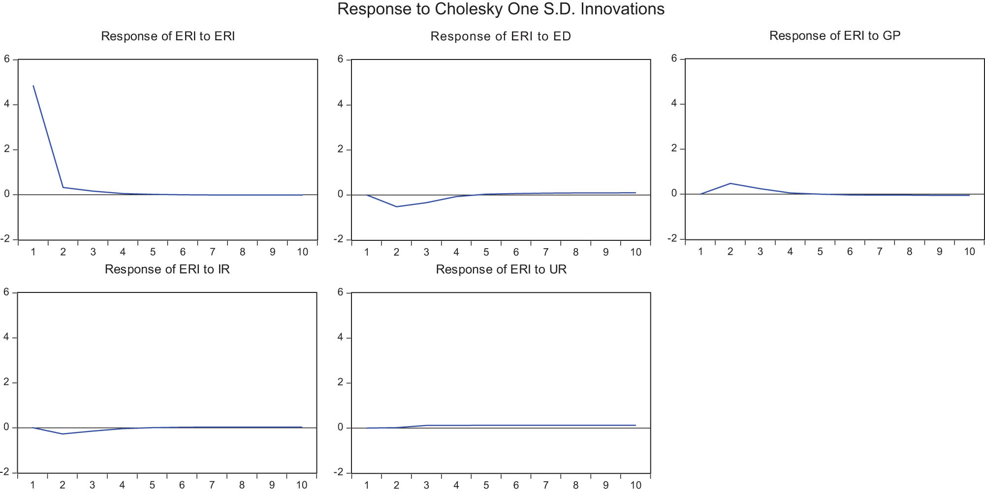
4.5 Dynamics of Type V Areas
The self-shock impact caused by a change in ecological risk (ERI) presents the characteristics of positive change. It shows a positive impact but decreases sharply from periods 1–2, but its positive volatility gradually decreases from period 2 to period 4. Then, it has a small positive fluctuation and has been showing a stable trend after the fourth period (Figure 10).
Impulsive response of ERI to other variables in type V.
The disturbance effect of change in economic growth (ED) on the ecosystem (ERI) shows a positive divergent trend. It has a smaller positive perturbation effect in the first to third period, but its perturbation effect becomes larger during the third to the seventh period and becomes larger after the seventh period. Although it produces a relatively small positive disturbance and presents a relatively stable state in stages, it exhibits divergence (Figure 10).
Ecosystem (ERI) disturbances caused by green policy (GP) change are not significant. It produces a slight negative perturbation effect from period 1 to period 4 and always converges to its mean starting from period 4 (Figure 10).
The development of the secondary industry (IR) has always a negative disturbing effect on the ecological environment system (ERI). Its negative perturbation effect tends to increase from the first to the second period, while the negative perturbation effect gradually becomes smaller in the second to the fourth period. Further, its negative perturbation effect is small after the fifth period, and it has been showing a stable trend (Figure 10).
The disturbance effect of urbanization development (UR) on the ecological environment (ERI) shows a gradually increasing negative change from the first to the second period, but its negative change gradually becomes smaller after the second period. But since period 3, it has been converging to its mean (Figure 10).
4.6 Dynamics of Type VI Areas
In the Type VI areas, the self-shock impact caused by a change in ecological risk (ERI) presents the characteristics of positive and negative change. It shows a positive effect and decreases sharply from periods 1 to 2, but the positive fluctuation gradually decreases from period 2 to period 4. It starts to fluctuate from positive to negative after period 4, but the magnitude of negative fluctuation is smaller and has been showing a stable trend (Figure 11).
Impulsive response of ERI to other variables in type VI.
The disturbance effect of economic growth (ED) change on the ecosystem (ERI) presents alternately negative and positive features. It shows a gradually increasing trend of negative perturbation in the first to second period, but its negative perturbation effect gradually becomes smaller in the second to fourth period. Then, the disturbance effect changes from negative to positive from the fourth period, and has a gradually increasing trend. However, its positive perturbation effect appears to be relatively stable after the sixth period (Figure 11).
For Type VI regions, the disturbance to the ecosystem (ERI) caused by green policy (GP) changes is complex. It produces a progressively larger positive disturbance during periods 1–2, but the positive disturbance begins to decrease from periods 2–4. Then, its perturbation effect changes from positive to negative starting from period 4 and shows a divergent trend (Figure 11).
The disturbance effect of the development of the secondary industry (IR) on the ecological environment system (ERI) presents a state of negative and positive change. It produces a gradually increasing negative perturbation effect during the period 1 to 2, but its negative perturbation effect gradually becomes smaller in the periods 2 to 4. However, its perturbation effect changes from negative to positive after the fourth period and has been showing a stable trend after the fifth period (Figure 11).
The disturbance effect of urbanization development (UR) on the ecological environment (ERI) is always in a positive state. Its positive fluctuation range is not significant from the first period to the second period, but its positive change is more significant after the second period and shows a relatively stable trend (Figure 11).
4.7 Dynamics of Type VII Areas
In the Type VII areas, the self-shock impact caused by a change in ecological risk (ERI) presents a positive disturbance. Its positive fluctuation decreases sharply in periods 1–2, but gradually decreases in periods 2 to 3. However, its positive perturbation amplitude becomes small after the third period and has been showing a stable trend (Figure 12).
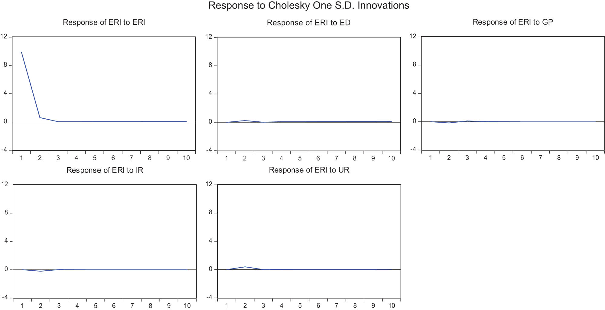
Impulsive response of ERI to other variables in type VII.
Change in economic growth (ED) has a positive disturbing effect on the ecosystem (ERI). Its positive perturbation effect is relatively large in the first to second period, but its positive perturbation effect is not significant during the second to third period. From the third period onwards, the positive perturbation effect slightly increases and shows a relatively stable state (Figure 12).
The disturbances caused by green policy (GP) change to the ecosystem (ERI) alternate negatively and positively. It produces a small negative perturbation effect from period 1 to period 2, but produces an insignificant positive perturbation effect from period 2 and almost converges to its mean (Figure 12).
The disturbance of the secondary industry development (IR) to the ecological environment system (ERI) is relatively small. It produces a relatively significant negative perturbation effect from period 1 to period 2, but the negative perturbation effect is small from period 2 and almost converges to its mean (Figure 12). This can be related to the industrial backwardness of the region.
The disturbance effect of urbanization development (UR) on the ecological environment (ERI) is in a positive state. Its positive fluctuation range is relatively large from period 1 to period 2, but its positive change is not significant after period 2 and almost converges to its mean value (Figure 12).
5 Discussion
The composite environmental risk index model constructed here is based on the mixed data of a specific combination of time and space effect. If it is only a single individual, we can assume that the spatial factor effect is zero (Dou, 2022). In addition, this article uses the absolute deviation of individuals from their mean to measure risk. In fact, we can also define other Loss functions to measure risk according to different research objects and purposes.
Our research object is China’s provincial administrative regions. Although China’s provincial administrative regions are independent regions, they are all in a unified market system. Therefore, there may be spatial spillover effects between different regions (Bai et al., 2023). However, as far as the composite environmental risk index model is concerned, it is fully applicable to research objects with countries as regions, as we use statistical means of sample cross-sections when calculating spatial factors for comparison and analysis. Generally, we do not need to consider the heterogeneity of sample individuals (spaces), as their weights are calculated using the same method. That is to say, the effects of organizational constraints and the spatial limits are not significant.
Our model measures the changes in the ecological environment (environmental risks). Therefore, we are considering environmental indicators such as water resources, natural disasters, waste discharge, and environmental governance investment. Of course, we can also quantify environmental changes (environmental risks) from the perspective of ecological environmental behavior, selecting indicators such as environmental concerns, social economic sequences, and environmental governance for quantitative analysis (Xu & Bao, 2023). However, it may be more suitable to choose environmental display indicators for measurement and evaluation for large distributed areas such as provincial-level regions in China.
There are many factors that lead to environmental risks. This article focuses on the role of economic growth, secondary industry, urbanization, and green policies. In fact, they can be further decomposed into more specific factors. Especially, green policies include many related policies (Li et al., 2023). In addition, different regions adopt different green policies. Due to the complexity of these issues, this article only provides a general analysis.
The results of the dynamic analysis of the regional environment system indicate that the effectiveness of China’s environmental protection policies is significant. From the empirical results of at least seven types of regions we have divided, we can find that due to the implementation of strict environmental protection policies, the ecological environment conditions in each region are gradually stabilizing, but this does not mean that the environmental conditions in all regions of China have been completely improved. Due to the large area of China’s provincial-level regions, there are significant differences in the ecological environment conditions of different sub-regions within each provincial-level region. This may lead to differences in the conclusions compared to the intuitive perception of specific regions. To this end, regions can be divided into smaller areas for measurement and evaluation based on different research objectives and tasks.
6 Conclusion
The goal of this article is to construct an composite environment risk index to measure and evaluate the environmental risks of the regions in mainland China. The study finds that the risk index of each region shows significant and unstable changes during the 2004–2019 sample period, which indicates that the environment of these regions is at a greater risk. Further, we find that the environment of each province-level region in China has the following characteristics of changes. First of all, the environmental changes in most regions do not show significant and relatively stable phased characteristics. Second, the environment of most regions shows divergent changes. Finally, although the environmental protection policies and measures of the national and all regions have become stricter in recent years, the environmental risks have not been significantly improved.
This article empirically tests the impact of four key economic variables of economic growth, urbanization development, secondary industry growth, and green policy on the environment on the basis of environment risk measurement and evaluation. The study finds that economic growth, secondary industry growth, and green policies have a negative correlation with the environment risk index, while there is a positive correlation between urbanization development and the environment risk, which is in line with the actual situation in China. Although economic growth and the growth of the secondary industry have certain adverse effects on the environment, China has been implementing strict environmental protection policies in recent years and at the same time continuously increasing investment in environmental governance, thereby reducing the negative impact on the environment. Because the goal of green policies is to improve the environment, it has a positive impact on the environment. On the other hand, because China’s urbanization development is large-scale, rapid, and extensive, it has a direct negative impact on the environment.
The research results of this article show that although China’s regional environmental risks are still relatively large at this stage, China’s regional environmental risks will be controlled within a reasonable range with China’s social and economic development and the continuous implementation of environmental protection policies. The future regional environment governance should focus on the following aspects on the premise of solving social and economic problems and regional imbalances.
Full implementation of green policies. Because green policies have direct and significant effects on improving the environment, China must implement more stringent green policies in all areas of consumption, product and energy production, circulation, and urban infrastructure construction in the future (Yang et al., 2022).
Significantly increase capital investment in water resources and watershed management, biodiversity protection, and environment infrastructure (Crist et al., 2017; Moffette et al., 2021). The first is to increase financial investment in environmental governance. Because the environment has the attributes of public goods, the central and local governments must bear the corresponding governance and protection responsibilities. The second is to encourage social capital to participate in the governance and protection of the environment through financial and fiscal policies to make up for the lack of fiscal funds. With the increasing environmental awareness of the public and enterprises, the potential of social capital is huge.
Comprehensively to promote the development of high-quality urbanization. At this stage, China’s urbanization has achieved a large-scale quantitative expansion and has been in a stage of transition from a quantitative development to a qualitative development. Therefore, China must promote the high-quality development of cities in a timely manner. This is not only a requirement for the management and protection of the environment, but also an inevitable requirement for improving the efficiency of urban development.
The research provides a multi-index and comprehensive environment risk assessment method. The advantage of this method is that it can not only perform multi-index and multi-scale evaluation but also extract the spatial and temporal effects of the objects evaluated. Therefore, the results measured by such a method are conducive to objective evaluation from the vertical and horizontal dimensions. In addition, this method provides a methodological basis for risk measurement and evaluation of more complex systems, subsystems, and larger index systems.
Acknowledgments
The authors thank anonymous reviewers and editors for valuable comments and revision suggestions.
-
Funding information: The authors state no funding involved.
-
Conflict of interest: The authors state no conflict of interest.
-
Article note: As part of the open assessment, reviews and the original submission are available as supplementary files on our website.
References
Afridi, F., Sisir Debnath, S., & Somanathan, E. (2021). A breath of fresh air: Raising awareness for clean fuel adoption. Journal of Development Economics, 151, 102674.Suche in Google Scholar
Ahmed, Z., Asghar, M. M., Malik, M. N., & Nawaz, K. (2020). Moving towards a sustainable environment: The dynamic linkage between natural resources, human capital, urbanization, economic growth, and ecological footprint in China. Resource Policy, 67, 101677. doi: 10.1016/j.resourpol.2020.101677.Suche in Google Scholar
Bai, J., Guo, K. L., Liu, M. R., & Jiang, T. (2023). Spatial variability, evolution, and agglomeration of eco-environmental risks in the Yangtze River Economic Belt, China. Ecological Indicators, 152, 110375.Suche in Google Scholar
Bryan, B. A., Gao, L., Ye, Y. Q., Sun, X. F., Connor, J. D., Crossman, N. D., Stafford-Smith, M., Wu, J. G., He, C. Y., Yu, D. Y., Liu, Z. F., Li, A., Huang, Q. X., Ren, H., Deng, X. Z., Zheng, H., Niu, J. M., Han, G. D., & Hou, X. Y. (2018). China’s response to a national land-system sustainability emergency. Nature, 559, 193–204. doi: 10.1038/s41586-018-0280-2.Suche in Google Scholar
Cao, H. J., Qi, Y., Chen, J. W., Shao, S. A., & Lin, S. X. (2021). Incentive and coordination: Ecological fiscal transfers’ effects on eco-environmental quality. Environmental Impact Assessment Review, 87, 106518. doi: 10.1016/j.eiar.2020.106518.Suche in Google Scholar
Chen, C. F., Sun, Y. W., Lan, Q. X., & Jiang, F. (2020). Impacts of industrial agglomeration on pollution and ecological efficiency: A spatial econometric analysis based on a big panel dataset of China’s 259 cities. Journal of Cleaner Production, 258, 120721. doi: 10.1016/j.jclepro.2020.120721.Suche in Google Scholar
Crist, E., Mora, C., & Engelman, R. (2017). The interaction of human population, food production, and biodiversity protection. Science, 356, 260–264. doi: 10.1126/science.aal2011.Suche in Google Scholar
Dhiman, H. S., & Deb, D. (2020). Fuzzy TOPSIS and fuzzy COPRAS based multi-criteria decision making for hybrid wind farms. Energy, 202, 117755. doi: 10.1016/j.energy.2020.117755.Suche in Google Scholar
Dou, X. S. (2015). Food waste generation and its recycling recovery: China’s governance mode and its assessment. Fresenius Environmental Bulletin, 24, 1474–1482.Suche in Google Scholar
Dou, X. S. (2016). A critical review of groundwater utilization and management in China’s inland water shortage areas. Water Policy, 18, 1367–1383. doi: 10.2166/wp.2016.043.Suche in Google Scholar
Dou, X. S. (2022). Agro-ecological sustainability evaluation in China. Journal of Bioeconomics, 24, 223–239. doi: 10.1007/s10818-022-09325-3.Suche in Google Scholar
Ervural, B. C., Zaim, S., Demirel, O. F., Aydin, Z., & Delen, D. (2018). An ANP and fuzzy TOPSIS-based SWOT analysis for Turkey’s energy planning. Renewable & Sustainable Energy Reviews, 82, 1538–1550. doi: 10.1016/j.rser.2017.06.095.Suche in Google Scholar
González-González, A., Villegas, J. C., Clerici, N., & Salazar, J. F. (2021). Spatial-temporal dynamics of deforestation and its drivers indicate need for locally-adapted environmental governance in Colombia. Ecological Indicators, 126, 107695. doi: 10.1016/j.ecolind.2021.107695.Suche in Google Scholar
Halkos, G., & Argyropoulou, G. (2022). Using environmental indicators in performance evaluation of sustainable development health goals. Ecological Economics, 192, 107263. doi: 10.1016/j.ecolecon.2021.107263.Suche in Google Scholar
Kahn, M. E., Sun, W. Z., & Zheng, S. Q. (2022). Clean air as an experience good in urban China. Ecological Economics, 192, 107254. doi: 10.1016/j.ecolecon.2021.107254.Suche in Google Scholar
Kramer, J. S. (1991). The logit model for economists. London: Edward Arnold Publishers.Suche in Google Scholar
Lafortune, G., Fuller, G., Moreno, J., Schmidt-Traub, G., & Kroll, C. (2018). SDG Index and Dashboards: Methodology Paper. https://www.sustainabledevelopment.report/reports/.Suche in Google Scholar
Li, C., Xia, W. J., & Wang, L. P. (2023). Synergies of green policies and their pollution reduction effects: Quantitative analysis of China’s green policy texts. Journal of Cleaner Production, 412, 137360.Suche in Google Scholar
Li, X. F. (2021). TOPSIS model with entropy weight for eco geological environmental carrying capacity assessment. Microprocessors and Microsystems, 82, 103805. doi: 10.1016/j.micpro.2020.103805.Suche in Google Scholar
Li, Y. R., Zhang, X. C., Cao, Z., Liu, Z. J., Lu, Z. E., & Liu, Y. S. (2021). Towards the progress of ecological restoration and economic development in China’s Loess Plateau and strategy for more sustainable development. Science of the Total Environment, 756, 143676. doi: 10.1016/j.scitotenv.2020.143676.Suche in Google Scholar
Liu, B. S., Wang, T., Zhang, J. M., Wang, X. M., Chang, Y., Fang, D. P., Yang, M. J., & Sun, X. Z. (2021). Sustained sustainable development actions of China from 1986 to 2020. Scientific Reports, 11, 8008. doi: 10.1038/s41598-021-87376-8.Suche in Google Scholar
Liu, D., Qi, X. C., Fu, Q., Li, M., Zhu, W. F., Zhang, L. L., Faiz, M. A., Khan, M. I., Li, T. X., & Cui, S. (2019). A resilience evaluation method for a combined regional gricultural water and soil resource system based on weighted Mahalanobis distance and a Gray-TOPSIS model. Journal of Cleaner Production, 229, 667–679. doi: 10.1016/j.jclepro.2019.04.406.Suche in Google Scholar
Miola, A., & Schiltz, F. (2019). Measuring sustainable development goals performance: How to monitor policy action in the 2030 agenda implementation? Ecological Economics, 164, 106373. doi: 10.1016/j.ecolecon.2019.106373.Suche in Google Scholar
Moffette, F., Skidmore, M., & Gibbs, H. K. (2021). Environmental policies that shape productivity: Evidence from cattle ranching in the Amazon. Journal of Environmental Economics and Management, 109, 102490. doi: 10.1016/j.jeem.2021.102490.Suche in Google Scholar
National Bureau of Statistic. (2021). Annual Data. https://data.stats.gov.cn/index.htm. 2021-10-02.Suche in Google Scholar
Noori, A., Bonakdari, H., Salimi, A. H., & Gharabaghi, B. (2021). A group Multi-Criteria Decision-Making method for water supply choice optimization. Socio-Economic Planning Sciences, 77, 101006. doi: 10.1016/j.seps.2020.101006.Suche in Google Scholar
OECD. (2017). Measuring distance to the SDG targets: An assessment of where OECD countries stand. http://www.oecd.org/std/OECD-Measuring-Distance-to -SDG-Targets.pdf.Suche in Google Scholar
Palczewski, K., & Sałabun, W. (2019). The fuzzy TOPSIS applications in the last decade. Procedia Computer Science, 159, 2294–2303. doi: 10.1016/j.procs.2019.09.404.Suche in Google Scholar
Qin, M., Sun, M. X., & Li, J. (2021). Impact of environmental regulation policy on ecological efficiency in four major urban agglomerations in eastern China. Ecological Indicators, 130, 108002. doi: 10.1016/j.ecolind.2021.108002.Suche in Google Scholar
Sachs, J., Schmidt-Traub, G., Kroll, C., Lafortune, G., & Fuller, G. (2018). SDG index and dashboards report 2018. New York: Bertelsmann Stiftung and Sustainable Development Solutions Network (SDSN). https://www.sustainabledevelopment.report/reports/sdg-index-and-dashboards-2018/.Suche in Google Scholar
Sachs, J., Schmidt-Traub, G., Kroll, C., Lafortune, G., & Fuller, G. (2021). Sustainable development report 2021: The decade of action for the sustainable development goals. Cambridge University Press. doi: 10.1017/9781009106559.Suche in Google Scholar
Schmidt-Traub, G., Kroll, C., Teksoz, K., Durand-Delacre, D., & Sachs, J. D. (2017). National baselines for the sustainable development goals assessed in the SDG Index and ashboards. Nature Geoscience, 10, 547–556. doi: 10.1038/NGEO2985.Suche in Google Scholar
Shi, L. D., & Moser, S. (2021). Transformative climate adaptation in the United States: Trends and prospects. Science, 372, 8054. doi: 10.1126/science.abc8054.Suche in Google Scholar
Shi, T., Yang, S. Y., Zhang, W., & Zhou, Q. (2020). Coupling coordination degree measurement and spatiotemporal heterogeneity between economic development and ecological environment: Empirical evidence from tropical and subtropical regions of China. Journal of Cleaner Production, 244, 118739. doi: 10.1016/j.jclepro.2019.118739.Suche in Google Scholar
Streimikiene, D., & Kyriakopoulos, G. L. (2023). Energy poverty and low carbon energy transition. Energies, 16, 610.Suche in Google Scholar
Streimikiene, D., Kyriakopoulos, G. L., Lekavicius, V., & Siksnelyte-Butkiene, I. (2021). Energy poverty and low carbon just energy transition: Comparative study in lithuania and greece. Social Indicators Research, 158, 319–371. doi: 10.1007/s11205-021-02685-9 Suche in Google Scholar
Streimikiene, D., Lekavičius, V., Baležentis, T., Kyriakopoulos, G. L., & Abrhám, J. (2020). Climate change mitigation policies targeting households and addressing energy poverty in european union. Energies, 13, 3389.Suche in Google Scholar
United Nations. (2015a). Transforming our world: the 2030 agenda for sustainable development. https://sustainabledevelopment.un.org/post2015/transformingourworld/publication.Suche in Google Scholar
United Nations. (2015b). Sustainable Development Goals: 17 Goals to Transform Our World. http://www.un.org/sustainabledevelopment/sustainable-development-goals/.Suche in Google Scholar
United Nations. (2021). The Sustainable Development Goals Report 2021. https://unstats.un.org/sdgs/report/2021/.Suche in Google Scholar
Xu, M. T., & Bao, C. (2023). Unveiling the comprehensive resources and environmental effciency and its influencing factors: Within and across the five urban agglomerations in Northwest China. Ecological Indicators, 154, 110466.Suche in Google Scholar
Xu, Z. C., Chau, S. N., Chen, X. Z., Zhang, J., Li, Y. J., Dietz, T., Wang, J. Y., Winkler, J. A., Fan, F., Huang, B. R., Li, S. X., Wu, S. H., Herzberger, A., Tang, Y., Hong, D. Q., Li, Y. K., & Liu, J. G. (2020). Assessing progress towards sustainable development over space and time. Nature, 577, 74–78. doi: 10.1038/s41586-019-1846-3.Suche in Google Scholar
Yang, Q. Y., Gao, D., Song, D. Y., & Li, Y. (2021). Environmental regulation, pollution reduction and green innovation: The case of the Chinese water ecological civilization city pilot policy. Economic Systems, 45, 100911. doi: 10.1016/j.ecosys.2021.100911. Suche in Google Scholar
Yang, Y. F., Wang, H., Loschel, A., & Zhou, P. (2022). Patterns and determinants of carbon emission flows along the Belt and Road from 2005 to 2030. Ecological Economics, 192, 107260. doi: 10.1016/j.ecolecon.2021.107260.Suche in Google Scholar
Yao, J. D., Xu, P. P., & Huang, Z. J. (2021). Impact of urbanization on ecological efficiency in China: An empirical analysis based on provincial panel data. Ecological Indicators, 129, 107827. doi: 10.1016/j.ecolind.2021.107827.Suche in Google Scholar
Zhang, R. L., & Liu, X. H. (2021). Evaluating ecological efficiency of Chinese industrial enterprise. Renewable Energy, 178, 679–691. doi: 10.1016/j.renene.2021.06.119.Suche in Google Scholar
© 2023 the author(s), published by De Gruyter
This work is licensed under the Creative Commons Attribution 4.0 International License.
Artikel in diesem Heft
- Regular Articles
- Export Cutoff Productivity, Uncertainty and Duration of Waiting for Exporting
- Survival of the Fittest: The Long-run Productivity Analysis of the Listed Information Technology Companies in the US Stock Market
- A Replication of “The Effect of the Conservation Reserve Program on Rural Economies: Deriving a Statistical Verdict from a Null Finding” (American Journal of Agricultural Economics, 2019)
- An Alternative Approach to Frequency of Patent Technology Codes: The Case of Renewable Energy Generation
- Environmental Taxation and International Trade in a Tax-Distorted Economy
- Foreign Investors and the Peer Effects to Payout Policies
- Segregation, Education Cost, and Group Inequality
- Does the Different Ways of Internet Utilization Promote Entrepreneurship: Evidence from Rural China
- Reinvestigating the U.S. Consumption Function: A Nonlinear Autoregressive Distributed Lags Approach
- Regional Environment Risk Assessment Over Space and Time: A Case of China
- Unraveling Producer Price Inflation Pass-Through: Quantification, Structural Breaks, and Causal Direction
- The Relationship Between Knowledge Risk Management and Sustainable Organizational Performance: The Mediating and Moderating Role of Leadership Behavior
- Special Issue: Data Governance in the Digital Era
- From Competition Law to Platform Regulation – Regulatory Choices for the Digital Markets Act
- IP Law and Policy for the Data Economy in the EU
- Is Data the New Gold? Considering Intellectual Property Protection and Regulation of Data
- Special Issue: Shapes of Performance Evaluation in Economics and Management Decision - Part I
- Path Constitution: Building Organizational Resilience for Sustainable Performance
- An Evaluation of E7 Countries’ Sustainable Energy Investments: A Decision-Making Approach with Spherical Fuzzy Sets
- Special Issue: Economic Implications of Management and Entrepreneurship - Part I
- Organizational Integration, Knowledge Management, and Sustainable Entrepreneurship for SMEs in Developing Economies
- Does Bitcoin Affect Term Deposits? Evidence from MINT Countries
- Effects of Social Responsibility Practices on the Brand Image, Brand Awareness, and Brand Loyalty of Sponsor Businesses: A Study on Sports Clubs
- The Effect of Market and Technological Turbulence on Innovation Performance in Nascent Enterprises: The Moderating Role of Entrepreneur’s Courage