Dependence properties of bivariate copula families
-
Jonathan Ansari


Abstract
Motivated by recently investigated results on dependence measures and robust risk models, this article provides an overview of dependence properties of many well known bivariate copula families, where the focus is on the Schur order for conditional distributions, which has the fundamental property that minimal elements characterize independence and maximal elements characterize perfect directed dependence. We give conditions on copulas that imply the Schur ordering of the associated conditional distribution functions. For extreme-value copulas, we prove the equivalence of the lower orthant order, the Schur order for conditional distributions, and the pointwise order of the associated Pickands dependence functions. Furthermore, we provide several tables and figures that list and illustrate various positive dependence and monotonicity properties of copula families, in particular, from classes of Archimedean, extreme-value, and elliptical copulas. Finally, for Chatterjee’s rank correlation, which is consistent with the Schur order for conditional distributions, we give some new closed-form formulas in terms of the parameter of the underlying copula family.
1 Introduction
In recent years, there is an increasing number of scientific articles on dependence measures (a.k.a. measures of predictability or measures of regression dependence), i.e., on functionals
which takes a simple form, has a fast estimator, and allows interesting applications, such as a model-free, dependence-based forward feature selection (see [4,12–14]). A large class of measures of predictability
Characterization of independence:
Characterization of perfect directed dependence:
Consistency with
The Schur order for conditional distributions and so Chatterjee’s rank correlation, which both can be extended to multivariate vectors of input variables, are merely rank-based concepts and depend in the case of continuous marginal distributions only on the underlying copula. More precisely, they are fully described by stochastically increasing[1] bivariate copulas, for which a pointwise comparison is equivalent to the comparison in the sense of the Schur order (see [4, Proposition 3.4]).
The Schur order for conditional distributions also applies to recently studied comparison results for ∗-products of several bivariate copulas modeling the dependence structure of conditionally independent factor models. Comparison results for large classes of such models with respect to the strong notion of supermodular order are given in [7] allowing applications in risk analysis when some structural assumptions on the underlying distribution are imposed. Risk bounds for these models are specified by a set of marginal distributions and a set of stochastically increasing or
Motivated by the above-mentioned applications, in this article, we investigate positive dependence and ordering properties for members of various well known bivariate copula families with the aim to provide a concise overview of their dependence properties. More specifically, we determine for copulas, in particular from classes of Archimedean, extreme-value, and elliptical distributions, whether they are conditionally increasing/decreasing,
The remainder of this article is organized as follows: Section 2 provides the necessary tools for analyzing bivariate dependencies. In Section 3, we focus on ordering results with respect to the Schur order for conditional distributions and provide several tables and figures that give a concise overview of the dependence properties of more than 35 bivariate copula families. The often tedious calculations are all deferred to Appendix.
2 Basic concepts of dependence modeling
In this section, we provide the main tools for modeling bivariate dependence structures. First, we give the definition of a copula and consider the well known classes of Archimedean, extreme-value, and elliptical copulas. Then, we introduce the stochastic orderings and dependence concepts which we make use of. Finally, we consider some specific measures of association. For multivariate extensions of all these concepts, we refer to the literature on dependence modeling (see, e.g., [19,47]).
2.1 Copulas
A bivariate copula is a function
The copula
2.1.1 Archimedean copulas
Let
is a bivariate copula if and only if
2.1.2 Extreme-value copulas
Let
(see, e.g., [19, Theorem 6.6.7]). We study dependence properties of several extreme-value copula families in Section 3.1.2.
2.1.3 Elliptical copulas
A bivariate random vector
The random vector
where
2.2 Stochastic orderings
For comparing dependencies, orderings on the set of copulas are useful. In the first part of this section, we consider the lower orthant (i.e., the pointwise) ordering of copulas. In the second part, we introduce to the recently studied rearrangement-based orderings of copulas.
2.2.1 Orthant orderings
The certainly most popular ordering on the set of bivariate copulas is the lower orthant order, which is defined by the pointwise comparison of bivariate copulas as follows.
Definition 2.1
(Lower orthant order) Let
The uniquely determined maximal and minimal elements in the class of bivariate copulas are the upper and lower Fréchet copula
(see, e.g., [19]). Furthermore, the upper orthant order on
As an immediate consequence of (4), for bivariate copulas, the lower and upper orthant orders are equivalent. Hence, the in the literature frequently considered concordance order, which is defined through the lower and upper orthant ordering of copulas, coincides for bivariate copulas with the lower orthant order. Note that in the three- and higher-dimensional setting, the lower and upper orthant orders diverge (see [46]).
2.2.2 Orderings of predictability
Due to axiom (A2), an ordering of predictability should be invariant with respect to bijective transformations of the input variable
where
Denote by
Definition 2.2
(Schur order for conditional distributions) Let
Due to (6), the Schur order in the aforementioned definition compares the variability of conditional distribution functions in the conditioning variable with respect to the Schur order for functions (Figure 1). Since minimal elements of the Schur order for functions in (5) are constant functions, it follows that minimal elements with respect to the Schur order for conditional distributions are independent random vectors. Similarly, for bounded functions, maximal elements in the Schur order for functions attain essentially two values given by the bounds. It follows that maximal elements with respect to the Schur order for conditional distributions are perfectly directed dependent random vectors (see [4, Theorem 3.5]). As shown in [5], the Schur order for conditional distributions satisfies the axioms (A1)–(A3) for a large class of functionals

Variability of conditional distribution functions described by the decreasing rearrangements (right) of the copula derivatives
In the case of continuous marginal distribution functions, the copula
for all
This motivates to define a version of the Schur order for conditional distributions considering derivatives of bivariate copulas as follows [3,6,56].
Definition 2.3
(Schur order for copula derivatives) Let
We write
Since constant functions are minimal with respect to the Schur order for functions, the independence copula
As discussed earlier, the Schur order for conditional distributions and the Schur order for copula derivatives coincide in the following sense.
Lemma 2.4
(Characterization of the Schur orderings) Let D and E be bivariate copulas, and let
Under some positive dependence assumptions on the underlying distributions, the lower orthant order and the Schur order for conditional distributions are equivalent, as we discuss in the following subsection.
2.3 Positive and negative dependence concepts
Many members of the well known bivariate copula families exhibit positive or negative dependencies. We make use of the following positive dependence concepts.
Definition 2.5
(Positive dependence concepts) A bivariate random vector
positive lower orthant dependent (PLOD) if
conditionally increasing in sequence (CIS) if
conditionally increasing (CI) if
totally positive of order 2 (
For continuous marginal distribution functions, the terms in the aforementioned definition depend only on the underlying copula, so we also refer the definition to copulas. The concepts are related by
where all implications are strict (see [46, page 146] for an overview of these concepts). The following lemma relates the lower orthant order and the Schur order for copula derivatives under some positive dependence conditions (see [6, Lemma 3.16]).
Lemma 2.6
Let D and E be the bivariate copulas. Then, the following statements hold true:
If E is CIS, then
If D and E are CIS, then
The Schur order for conditional distributions generates large subclasses of distributions for which the extremal elements with respect to the lower orthant order are CIS. To be more precise, consider for a bivariate copula
Lemma 2.7
(Extremal elements in
There exist a uniquely determined minimal copula
The copula
Lemma 2.8
Let D and E be the bivariate copulas. Then, the following statements hold true:
If E is CDS, then
If D and E are CDS, then
As we list in Tables 3 and 5, many well known copulas are CI or CD and thus coincide with their increasing rearranged copula
2.4 Measures of association
In this section, we consider some well known measures of association. While Spearman’s rho, Kendall’s tau, and the tail-dependence coefficients are consistent with the lower orthant order, Chatterjee’s rank correlation is consistent with the Schur order for conditional distributions.
2.4.1 Measures of concordance
Let
where
Both measures fulfil the axioms of a measure of concordance and are, in particular, consistent with the pointwise ordering of copulas as follows (see, e.g., [19, Theorem 2.4.9]).
Lemma 2.9
(Consistency with
2.4.2 Measures of predictability
For a bivariate random vector
A recently studied measure of predictability that has attracted a lot of attention is Chatterjee’s rank correlation
Lemma 2.10
(Consistency with
If
(see, e.g., [24]). Due to Lemmas 2.4 and 2.10, for bivariate copulas
2.4.3 Tail dependence
Further classical measures of association for bivariate copulas are the tail-dependence coefficients, which are defined as follows (see, e.g., [38,47]).
Definition 2.11
(Tail-dependence coefficients) Let
and the upper tail-dependence coefficient of
The following lemma is immediate from the definition of the tail-dependence coefficient.
Lemma 2.12
(Consistency with
3 Dependence properties of bivariate copula families
As motivated in Section 1, in this section, we study various dependence properties of bivariate copula families that are often used in applications. More precisely, we consider the families listed in Table 1. For each copula family, we verify or refer for which parameters the copulas are CI, CD, or
Overview of Archimedean (Arch.), extreme-value (EV), elliptical (Ell.), and unclassified (Uncl.) copula families for which dependence properties are studied in this article
| Family | Notation | Copula
|
|
|---|---|---|---|
| Arch. | Clayton |
|
|
| Nelsen2 |
|
|
|
| Ali-Mikh.-Haq |
|
|
|
| Gumbel-Hougaard |
|
|
|
| Frank |
|
|
|
| Joe |
|
|
|
| Nelsen7 |
|
|
|
| Nelsen8 |
|
|
|
| Gumb.-Barn. |
|
|
|
| Nelsen10 |
|
|
|
| Nelsen11 |
|
|
|
| Nelsen12 |
|
|
|
| Nelsen13 |
|
|
|
| Nelsen14 |
|
|
|
| Genest-Ghoudi |
|
|
|
| Nelsen16 |
|
|
|
| Nelsen17 |
|
|
|
| Nelsen18 |
|
|
|
| Nelsen19 |
|
|
|
| Nelsen20 |
|
|
|
| Nelsen21 |
|
|
|
| Nelsen22 |
|
|
|
| EV | BB5 |
|
|
| Cuadras-Augé |
|
|
|
| Galambos |
|
|
|
| Gumbel-Hougaard |
|
|
|
| Hüsler-Reiss |
|
|
|
| where
|
|||
| Joe-EV |
|
|
|
| Marshall-Olkin |
|
|
|
| t-EV |
|
|
|
| where
|
|||
| EV | Tawn |
|
|
| Ell. | Gaussian |
|
|
| Student-t |
|
|
|
| Laplace |
|
|
|
| Uncl. | Fréchet |
|
|
| Mardia |
|
|
|
| Farl.-Gumb.-Morg. |
|
|
|
| Plackett |
|
|
|
| Raftery |
|
|
The Gumbel-Hougaard family also belongs to the class of EV copula families.
Overview of Archimedean copula families, for which dependence properties are given in Table 3
| Family |
|
|
Generator
|
Inverse generator
|
Special/limiting cases |
|---|---|---|---|---|---|
| Clayton |
|
|
|
|
|
| else
|
|
||||
| Nelsen2 |
|
1 |
|
|
|
| AMH |
|
|
|
|
|
|
|
|||||
| Gum.-Ho. |
|
|
|
|
|
| Frank |
|
|
|
|
|
|
|
|||||
| Joe |
|
|
|
|
|
| Nelsen7 |
|
|
|
|
|
|
|
|||||
| Nelsen8 |
|
1 |
|
|
|
| Gum.-Ba. |
|
|
|
|
|
| Nelsen10 |
|
|
|
|
|
| Nelsen11 |
|
|
|
|
|
| Nelsen12 |
|
|
|
|
|
| Nelsen13 |
|
|
|
|
|
| Nelsen14 |
|
|
|
|
|
| Gen.-Gh. |
|
1 |
|
|
|
| Nelsen16 |
|
|
|
|
|
| else
|
|
|
|||
| Nelsen17 |
|
|
|
|
|
| Nelsen18 |
|
|
|
|
|
| Nelsen19 |
|
|
|
|
|
| Nelsen20 |
|
|
|
|
|
| Nelsen21 |
|
1 |
|
|
|
|
|
|||||
| Nelsen22 |
|
|
|
|
|
The generators are taken from [47, Table 3.2]. Generator and inverse generator for
Dependence properties of Archimedean copula families from Table 2
| Family | CI/CD |
|
|
|
|
|
|---|---|---|---|---|---|---|
| Clayton | ↑ iff
|
✓ iff
|
↗ | ↗ if
|
|
0 |
| ↓ iff
|
↘ if
|
|||||
| Nelsen2 | ✗ iff
|
✗ | ↗ | ✗* | 0 |
|
| Ali-Mikhail-Haq | ↑ iff
|
✓ iff
|
↗ | ↗ if
|
0 | 0 |
| ↓ iff
|
↘ if
|
|||||
| Gumbel-Hougaard | ↑ | ✓ | ↗ | ↗ | 0 |
|
| Frank | ↑ iff
|
✓ iff
|
↗ | ↗ if
|
0 | 0 |
| ↓ iff
|
↘ if
|
|||||
| Joe | ↑ | ✓ | ↗ | ↗ | 0 |
|
| Nelsen7 | ↓ | ✗ iff
|
↗ | ↘ | 0 | 0 |
| Nelsen8 | ✗ iff
|
✗ | ↗ | ✗* | 0 | 0 |
| Gumbel-Barnett | ↓ | ✗ iff
|
↘ | ↗ | 0 | 0 |
| Nelsen10 | ↓ | ✗ iff
|
✗ | ✗ | 0 | 0 |
| Nelsen11 | ↓ | ✗ iff
|
↘ | ↗ | 0 | 0 |
| Nelsen12 | ↑ | ✓ | ↗ | ↗ |
|
|
| Nelsen13 | ↑ iff
|
✓ iff
|
↗ | ↗ if
|
0 | 0 |
| Nelsen14 | ↑ | ✓ | ↗ | ↗ | 1/2 |
|
| Genest-Ghoudi | ✗ iff
|
✗ | ↗ | ✗* | 0 |
|
| Nelsen16 | ↑ iff
|
✓ iff
|
↗ | ↗ if
|
1/2 | 0 |
| Nelsen17 | ↑ iff
|
✓ iff
|
↗ | ↗ if
|
0 | 0 |
| ↓ iff
|
↘ if
|
|||||
| Nelsen18 | ✗ | ✗ | ↗ | ✗* | 0 | 1 |
| Nelsen19 | ↑ | ✓ | ↗ | ↗ | 1 | 0 |
| Nelsen20 | ↑ | ✓ | ↗ | ↗ | 1 | 0 |
| Nelsen21 | ✗ iff
|
✗ | ↗ | ✗* | 0 |
|
| Nelsen22 | ↓ | ✗ iff
|
↘ | ↗ | 0 | 0 |
For example, “↑ iff
Overview of elliptical, extreme-value, and unclassified copula families, for which dependence properties are given in Table 5
| Type | Family | Parameters | Pickands dependence function
|
Special/limiting cases |
|---|---|---|---|---|
| EV | BB5 |
|
|
|
|
|
|
|||
| Cuad.-Au. |
|
|
|
|
| Galambos |
|
|
|
|
| Gum.-Hou. |
|
|
|
|
| Hüsl.-Rei. |
|
|
|
|
|
|
||||
| Joe-EV |
|
|
|
|
|
|
|
|||
|
|
||||
|
|
||||
| Marsh.-Ol. |
|
|
|
|
| Tawn |
|
|
|
|
|
|
|
|
||
|
|
||||
| t-EV |
|
|
|
|
|
|
|
|||
| Ellip. | Gaussian |
|
— |
|
|
|
||||
| Student-t |
|
— |
|
|
|
|
||||
| Laplace |
|
— |
|
|
| Uncl. | Fréchet |
|
— |
|
|
|
||||
| Mardia |
|
— |
|
|
|
|
||||
| FGM |
|
— |
|
|
| Plackett |
|
— |
|
|
|
|
||||
| Raftery |
|
— |
|
Copula family properties for elliptical, extreme-value, and unclassified copulas, where
| Type | Family | CI/CD |
|
|
|
|
|
|---|---|---|---|---|---|---|---|
| EV | BB5 | ↑ | ? | ↗ in
|
↗ in
|
0 |
|
| Cua.-Au. | ↑ | ✗ iff
|
↗ | ↗ |
|
|
|
| Galambos | ↑ | ? | ↗ | ↗ | 0 |
|
|
| Gum.-Ho. | ↑ | ✓ | ↗ | ↗ | 0 |
|
|
| Hüsl.-Re. | ↑ | ✓
|
↗ | ↗ | 0 |
|
|
| Joe-EV | ↑ | ✗* iff
|
↗ in
|
↗ in
|
0 |
|
|
| Mar.-Ol. | ↑ | ✗ iff
|
↗ in | ↗ in |
|
|
|
| ✗* iff
|
|
|
|||||
| Tawn | ↑ | ✗* iff
|
↗ in
|
↗ in
|
0 |
|
|
|
|
|||||||
| t-EV | ↑ | ✗* | ↗ in
|
↗ in
|
|
|
|
| Ell. | Gauss | ↑ iff
|
✓ iff
|
↗ | ↗ if
|
|
|
| ↓ iff
|
↘ if
|
||||||
| Student-t | ✗ | ✗ | ↗ in
|
? |
|
|
|
| Laplace | ✗ if
|
✗ | ↗ | ? | ? | ? | |
| Uncl. | Fréchet | ↑ iff
|
✗ iff | ↗ in | ↗ for |
|
|
| ↓ iff
|
|
|
|
||||
| Mardia | ↑ iff
|
✗ iff
|
✗ | ↗
|
|
|
|
| ↓ iff
|
↘
|
||||||
| FGM | ↑ iff
|
✓ iff
|
↗ | ↗ if
|
0 | 0 | |
| ↓ iff
|
↘ if
|
||||||
| Plackett | ↑ iff
|
✗ if
|
↗ | ↗ if
|
0 | 0 | |
| ↓ iff
|
✓
|
↘ if
|
|||||
| Raftery | ↑ | ✗ iff
|
↗ | ↗ |
|
0 |
Results marked with * are obtained from numerical checks and neither referenced nor proved.
In order to verify the dependence properties, we provide in the following subsection sufficient positive/negative dependence and ordering conditions for the families from the respective classes of copulas. As we study in Section 3.2, various ordering properties imply monotonicity of Chatterjee’s xi, Spearman’s rho, and Kendall’s tau with respect to the parameter of the underlying copula family. We also provide some closed-form expressions for these measures in dependence on the copula parameter.
3.1 Ordering and positive dependence properties
While characterizations of the lower orthant order in terms of the generator or correlation parameter are well known for Archimedean and elliptical copula families (see Propositions 3.3(i) and 3.6(i)), we establish in Theorem 3.4 the equivalence between lower orthant ordering of extreme-value copulas and pointwise ordering of the associated Pickands dependence functions. For deriving ordering results with respect to the Schur order for copula derivatives, we make use of positive dependence properties for the respective classes of copulas. Before proceeding with the specific classes of copulas, we give two general results concerning the relation between the Schur order for copula derivatives and the lower orthant order as well as dependence properties for survival copulas.
The following result characterizes the Schur order for copula derivatives in terms of the pointwise ordering of the rearranged copulas. If a copula is CI, it coincides with its increasing rearranged copula. Hence, for families of CI copulas, the lower orthant order is equivalent to the Schur order for copula derivatives with respect to the first (and similarly to the second) component.
Proposition 3.1
(Rearranged copulas) For
Proof
Statement (1) is equivalent to
For a bivariate copula
(see, e.g., [19, Definition 1.7.18]). Due to the following result, all dependence and monotonicity properties in Tables 3 and 5 transfer to the associated survival copula families.
Proposition 3.2
(Survival copula) Let D and E be bivariate copulas. Then, the following statements hold true.
D is CIS if and only if
Proof
Since
Finally, to derive (iii), let
Since
3.1.1 Archimedean copulas
Positive dependence concepts for Archimedean copulas can be characterized in terms of their generators. For a bivariate Archimedean copula
(see [45, Theorems 2.8 and 2.11]). Since Archimedean copulas are symmetric, the concepts CIS and CI coincide. Concerning negative dependence, it follows similarly to the proof of [45, Theorems 2.8] that
We make use of the positive and negative dependence properties (13) and (15) to give sufficient conditions for the Schur ordering of bivariate Archimedean copula derivatives. To this end, a function
Proposition 3.3
(Ordering Archimedean copulas) Let
If
If
Proof
The first statement is a well known result given, e.g., in [47, Theorem 4.4.2]. For the second statement, note that the log-convexity of
3.1.2 Extreme-values copulas
The following theorem shows, on the one hand, the equivalence of the lower orthant order for bivariate extreme-value copulas and the reverse pointwise order of the associated Pickands dependence functions. On the other hand, since bivariate extreme-value copulas are always CI (see [29, Theorem 1]), we also obtain the equivalence of the reverse pointwise order for the Pickands dependence functions with the Schur order for conditional distributions and the Schur order for copula derivatives.
Theorem 3.4
(Ordering extreme-value copulas) Let
Proof
“
which shows
“
and hence,
“
“
“
“
Remark 3.5
For various well known families of extreme-value copulas, it can easily be verified that the associated Pickands dependence functions are pointwise ordered. Hence, Theorem 3.4 provides a simple characterization for ordering extreme-value copulas with respect to the lower orthant order and the Schur orders (see Table 5 and Figure 2). In particular, if the Pickands dependence functions are ordered, then Kendall’s tau, Spearman’s rho, the tail-dependence coefficients, and Chatterjee’s xi are reverse ordered (see Section 2.4). We refer to [9, 10] for a dependence ordering that is based on a probability transform and that is, for extreme-value copulas, strictly weaker than

Pickands dependence functions for the two-parametric BB5 and for the three-parametric Joe’s extreme-value copula family for some parameter choices. The Pickands functions are pointwise decreasing in their parameter. Hence, by Theorem 3.4, the BB5 and the Joe’s extreme-value copula family are increasing with respect to the lower orthant order and the Schur order for copula derivatives. The skewed Pickands dependence function for Joe’s extreme-value copula family reflects the fact that this copula family is not symmetric. For
3.1.3 Elliptical copulas
For the multivariate normal distribution, positive dependence concepts are characterized in terms of the correlation matrix [52]. More generally, for elliptical distributions, positive dependence properties also depend on the elliptical generator. In the case of bivariate elliptical distributions the
(see [1, Proposition 1.2]), where
Proposition 3.6
(Ordering elliptical copulas) Let
If g satisfies (16) for
Proof
The first statement is an immediate consequence of [38, Theorem 2.21]. For the second statement, consider first the case where
3.2 Monotonicity properties of measures of association
It is well known that Kendall’s tau, Spearman’s rho as well as the lower and upper tail-dependence coefficients are increasing with respect to the lower orthant order (Lemmas 2.9 and 2.12). By Lemmas 2.4 and 2.10, we know that Chatterjee’s rank correlation is increasing with respect to the Schur order for conditional distributions/copula derivatives. From Tables 3 and 5, we see that many well known bivariate copula families exhibit monotonicity properties with respect to the lower orthant order and the Schur order for copula derivatives. Consequently, these ordering properties explain the monotonicity of Kendall’s tau, Spearman’s rho and Chatterjee’s xi for many copula (sub-)families in Figures 3–6.[3]


Chatterjee’s xi, Spearman’s rho, and Kendall’s tau for the extreme-value copula families in Table 1. We consider special cases for multi-parameter families as stated in the
For example, we know from Table 3 that the Clayton copulas
We also see that Kendall’s tau, Spearman’s rho, and Chatterjee’s xi are all continuous in the underlying copula family parameters, which is a consequence of continuity of the copulas in their parameter with respect to uniform convergence and weak conditional convergence, respectively (see, e.g., [41]). In particular, if the underlying copulas converge to the lower/upper Fréchet copula, Kendall’s tau, and Spearman’s rho converge to
(see [47, Theorem 5.2.8]). The plots and simulations also suggest that

Chatterjee’s xi, Spearman’s rho, and Kendall’s tau for the elliptical copula families in Table 1. We consider
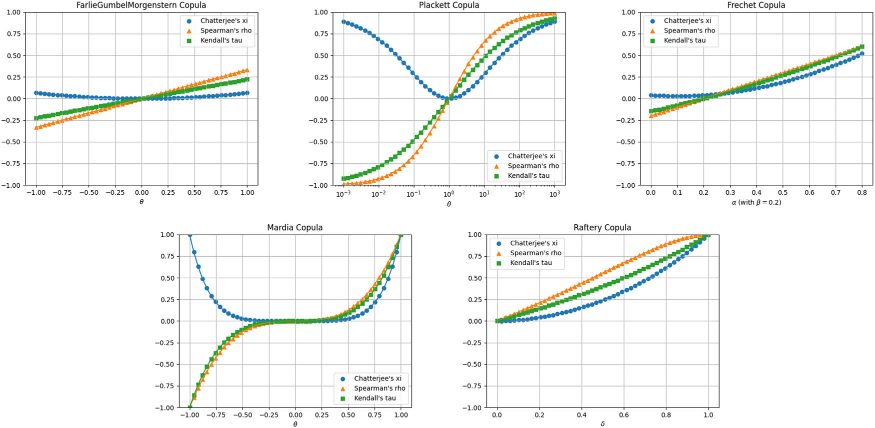
Chatterjee’s xi, Spearman’s rho, and Kendall’s tau for the unclassified copula families in Table 1. We consider
While closed-form expressions can easily be determined for the tail-dependence coefficients (see Tables 3 and Table 5), closed-form formulas are generally not applicable for Chatterjee’s rank correlation, Kendall’s tau, and Spearman’s rho. In Table 6, we give some expressions that allow for a fast calculation of the respective measures. Concerning Chatterjee’s rank correlation, the expressions for the Clayton, Ali-Mikail-Haq, Nelsen7, Marshall-Olkin (see [24, Example 4.2] for
Closed-form expressions if available for Chatterjee’s xi, Spearman’s rho, and Kendall’s tau for different copula families
| Type | Family | Chatterjee’s xi | Spearman’s rho | Kendall’s tau |
|---|---|---|---|---|
| Arch. | Clayton |
|
|
|
| AMH |
|
|
|
|
| Frank |
|
|
||
| Nelsen7 |
|
|
|
|
| Gumb.-Barn. |
|
|||
| EV | Cuadr.-Augé |
|
|
|
| Gumb.-Houg. |
|
|
||
| Marsh.-Olk. |
|
|
|
|
| Ellip. | Gaussian |
|
|
|
| Student-t |
|
|
||
| Laplace |
|
|
||
| Uncl. | Fréchet |
|
|
|
| Mardia |
|
|
|
|
| FGM |
|
|
|
|
| Plackett |
|
|||
| Raftery |
|
|
||
4 Conclusion
In this article, we have studied dependence properties of more than 35 well known copula families with the focus on the Schur order for conditional distributions, which is a rearrangement-invariant dependence order that is consistent with Chatterjee’s rank correlation. In Section 3, we have provided a comprehensive overview of the copula families and their dependence properties. Many of the considered copula families turn out to be Schur ordered either on the full parameter space or on a certain range of parameters (see Tables 3 and 5). Furthermore, for some copula families, we have derived new closed-form expressions of Chatterjee’s rank correlation.
Acknowledgements
Jonathan Ansari gratefully acknowledges the support of the Austrian Science Fund (FWF) Project P 36155-N ReDim: Quantifying Dependence via Dimension Reduction and the support of the WISS 2025 Project ‘IDA-lab Salzburg’ (20204-WISS/225/197-2019 and 20102-F1901166-KZP).
-
Author contributions: Both authors have accepted responsibility for the entire content of this manuscript and consented to its submission to the journal, reviewed all the results and approved the final version of the manuscript. JA conceived the manuscript and authored Sections 1 and 2. MR created the figures and tables, and performed the mathematical computations in the appendix. The authors collaboratively contributed to the theorem and propositions in Section 3.
-
Conflict of interest: The authors state no conflict of interest.
-
Data availability statement: Data sharing is not applicable to this article as no datasets were generated or analysed during the current study.
Appendix
In the sequel, we justify the properties in Tables 3, 5, and 6 either by computation or by providing references.
A.1 Computations for the Archimedean copula families in Table 3
The Gumbel-Hougaard copula family will be discussed in Subsection A.2, as this family is not only Archimedean but also an extreme-value copula family.
A.1.1 CI/CD and
TP
2
For the CI/CD and
Recall from (13) that a bivariate Archimedean copula with inverse generator
Clayton (
As we assumed
Nelsen2 (
so that PLOD fails to hold for any choice of
Ali-Mikhail-Haq (
Frank (
and
Nelsen7 (
which is trivially non-decreasing in
Nelsen8 (
In the case of
when
Gumbel-Barnett (
Nelsen10 (
Nelsen11 (
Since
Nelsen13 (
When
Genest-Ghoudi (
Substituting
Nelsen16 (
(A1)(A2)(A2) has roots for
Both factors of
Nelsen17 (
(A3)(A4)At
so for
and the right-hand side is indeed non-negative for
Nelsen18 (
Note also that for
which shows that PLOD fails to hold. On the other hand, the upper tail-dependence coefficient is strictly positive, so that also CD fails to hold.
Nelsen21 (
Then, for
Nelsen22 (
A.1.2 Lower orthant ordering and Schur ordering
The lower orthant (or, equivalently, concordance) order properties of the Archimedean copulas can be found in [47]. The families Ali-Mikhail-Haq, Frank, Joe, Nelsen7-8, Nelsen12-18, Nelsen20, and Nelsen21 are positively ordered by [47, Exercise 4.18 (a)], Clayton by [47, Exercise 4.14], Nelsen2 by [47, Exercise 4.23], and Nelsen19 by [47, Exercise 4.15]. Nelsen11 and Nelsen22 are negatively ordered by [47, Exercise 4.18 (b)] and Gumbel-Barnett by [47, Example 4.10]. Nelson10 is unordered by [47, Exercise 4.16].
Recall from Lemma 2.6 that when a copula is CI, then lower orthant ordering and Schur order are equivalent. Hence, the column on the Schur order in Table 3 is a direct consequence of the columns on CI and the lower orthant order. For those Archimedean copulas that are not CI/CD, we check the Schur ordering numerically by approximating the copulas with
A.1.3 Tail dependencies
Concerning the Archimedean copula families, the formulas for the lower and upper tail-dependence coefficients
A.2 Computations for the extreme-value copula families in Table 5
For the extreme-value copulas in Table 6, the associated Pickands dependence functions are given in Table 4. Note that the Marshall-Olkin extreme-value copula family yields the Cuadras-Augé copula family in the special case
A.2.1 CI/CD and
TP
2
Bivariate extreme-value copulas are always CI (see [29, Theorem 1]). The Marshall-Olkin copula is
A.2.2 Lower orthant ordering and Schur ordering
Due to Theorem 3.4, we only need to check whether Pickands dependence functions are on the interval
Galambos (
where
and hence, the same argument works here, showing that the Tawn copula family is positively ordered.
Gumbel-Hougaard (
Hüsler-Reiss (
Marshall-Olkin (
t-EV (
Second, the probability density function of the Student-t distribution with
Together, we obtain for the Pickands function that
(A5)(A6)(A5) is certainly non-positive as we assumed
Consequently,
A.2.3 Tail dependencies
The formulas for the upper tail-dependence coefficients are taken from [22, Table 3.2].
Lower tail-dependence coefficients are generally trivially given by
and the inequality is strict when
A.3 Computations for the elliptical copula families in Table 5
A.3.1 CI/CD and
TP
2
The Gauss copula is
A.3.2 Lower orthant ordering and Schur ordering
If the radial variable admits a Lebesgue density, then the copulas associated with a family of elliptical distributions are uniquely determined and by Proposition 3.6 (i)
A.3.3 Tail dependencies
When
(see [20, Section 5.3]).
A.4 Computations for the unclassified copula families in Table 5
Here, we discuss the Fréchet, Mardia, Farlie-Gumbel-Morgenstern, Plackett, and Raftery copula families, which are important examples for copula families that does not fit into the elliptical, Archmimedean, or extreme-value case.
A.4.1 CI/CD and
TP
2
The CI/CD and
Fréchet (
Mardia (
(A7)Likewise, CD holds if and only if
Farlie-Gumbel-Morgenstern (
is clearly non-increasing in
Plackett (
on
(A8)with
The denominator in (A8) is always positive, so we can focus on the positiveness of
Raftery (
(A9)The first expression in (A9) is non-increasing in
is negative for
A.4.2 Lower orthant ordering and Schur ordering
The Fréchet copula family is trivially lower orthant increasing when fixing either
A.4.3 Tail dependencies
The tail-dependence coefficients for the Fréchet copula family are found in, e.g., [47, Exercise 2.4]. From that, one obtains the tail-dependence coefficients for the Mardia copula family via (A7). The tail-dependence coefficients for the Plackett and Raftery copula families are found in, e.g., [47, Exercise 5.21]. Finally, the tail-dependence coefficients for the Farlie-Gumbel-Morgenstern copula family directly evaluate to
and likewise,
A.5 Computations for Chatterjee’s xi, Spearman’s rho, and Kendall’s tau in Table 6
In the sequel, we justify all entries in Table 6, either by reference or by computation. For the computations, we leverage the integral formulas given in (9), (10), and (11) above.
A.5.1 Archimedean copulas
In this subsection, we cover dependence measures for a number of Archimedean copula families, namely, the Clayton, Ali-Mikhail-Haq, Gumbel-Hougaard, Frank, Nelsen7, and Gumbel-Barnett copula families.
Clayton (
which satisfies
From this, one obtains
where
(A10)where
Ali-Mikhail-Haq (
from which we obtain for
As
Frank (
Nelsen7 (
and
In the limiting cases,
Gumbel-Barnett (
A.5.2 Extreme-value copula families
The formulas for Spearman’s rho and Kendall’s tau for the Gumbell-Hougaard copula family are found in [35, Example 4.2] and [47, Example 5.4]. For the Marshall-Olkin copula family, the formulas for Spearman’s rho and Kendall’s tau can be found, e.g., in [47, Example 5.7 a), Example 5.9 c)]. Chatterjee’s rank correlation
and for
Hence,
for all
for the Cuadras-Augé copula family as a special case.
A.5.3 Elliptical copula families
A general formula for Kendall’s tau of elliptical copulas is given in [20, Theorem 5.4]. The formula for Spearman’s rho for the Gaussian copula family can be found in [21, Theorem 5.36] or [32] and for the Student-t and Laplace copula families in [32, Proposition 1]. Note that [32, Proposition 4 and Remark 2] also give longer, more explicit formulas for Spearman’s rho of the Student-t and the Laplace copula families. The formula for Chatterjee’s xi in the Gaussian case is given, e.g., in [24, Example 4].
A.5.4 Unclassified copula families
The formulas for Spearman’s rho and Kendall s tau of unclassified copula families in Table 6 are given in [47, Example 5.2 and 5.7 a)] for the Farlie-Gumbel-Morgenstern, in [47, Example 5.3 and 5.6] for the Fréchet (and the Mardia), in [47, Exercise 5.8] for the Plackett, and in [47, Exercise 5.11] for the Raftery copula family.
The formulas for Chatterjee’s xi of unclassified copula families in Table 6 are given in [24, Example 4] for the Farlie-Gumbel-Morgenstern and the Fréchet coupla family, and from the latter one directly obtains the formula for the Mardia copula family.
References
[1] Abdous, B., Genest, C., & Rémillard, B. (2005). Dependence properties of meta-elliptical distributions. In Statistical Modeling and Analysis for Complex Data Problems (pp. 1–15), Boston (US): Springer. 10.1007/0-387-24555-3_1Suche in Google Scholar
[2] Amblard, C., & Girard, S. (2002). Symmetry and dependence properties within a semiparametric family of bivariate copulas. Journal of Nonparametric Statistics, 14(6), 715–727. 10.1080/10485250215322Suche in Google Scholar
[3] Ansari, J. (2019). Ordering risk bounds in partially specified factor models. Freiburg im Breisgau: Univ. Freiburg, Fakultät für Mathematik und Physik (Diss.). Suche in Google Scholar
[4] Ansari, J., & Fuchs, S. (2022). A simple extension of Azadkia and Chatterjee’s rank correlation to a vector of endogenous variables. arXiv: http://arXiv.org/abs/arXiv:2212.01621. Suche in Google Scholar
[5] Ansari, J., Langthaler, P. B., Fuchs, S., & Trutschnig, W. (2023). Quantifying and estimating dependence via sensitivity of conditional distributions. arXiv: http://arXiv.org/abs/arXiv:2308.06168. Suche in Google Scholar
[6] Ansari, J., & Rüschendorf, L. (2021). Sklaras theorem, copula products, and ordering results in factor models. Dependence Modeling, 9, 267–306. 10.1515/demo-2021-0113Suche in Google Scholar
[7] Ansari, J., & Rüschendorf, L. (2023). Supermodular and directionally convex comparison results for general factor models. Journal of Multivariate Analysis, 201, 105264. 10.1016/j.jmva.2023.105264Suche in Google Scholar
[8] Averous, J., & Dortet-Bernadet, J.-L. (2000). LTD and RTI dependence orderings. Canadian Journal of Statistics, 28(1), 151–157. 10.2307/3315794Suche in Google Scholar
[9] Capéraà, P., Fougères, A.-L., & Genest, C. (1997). A stochastic ordering based on a decomposition of Kendall’s tau. In Distributions with given Marginals and Moment Problems. Proceedings of the 1996 conference, Prague, Czech Republic (pp. 81–86). Dordrecht: Kluwer Academic Publishers. 10.1007/978-94-011-5532-8_9Suche in Google Scholar
[10] Capéraà, P., Fougères, A.-L., & Genest, C. (2000). Bivariate distributions with given extreme-value attractor. Journal of Multivariate Analysis, 72(1), 30–49. 10.1006/jmva.1999.1845Suche in Google Scholar
[11] Colangelo, A. (2008). A study on LTD and RTI positive dependence orderings. Statistics & Probability Letters, 78(14), 2222–2229. 10.1016/j.spl.2008.01.090Suche in Google Scholar
[12] Huang, Z., Deb, N., & Sen, B. (2022). Kernel partial correlation coefficient -Ť a measure of conditional dependence. Journal of Machine Learning Research, 23(216), 1–58. Suche in Google Scholar
[13] Chatterjee, S. (2020). A new coefficient of correlation. Journal of the American Statistical Association, 116(536), 2009–2022. 10.1080/01621459.2020.1758115Suche in Google Scholar
[14] Azadkia, M., & Chatterjee, S. (2021). A simple measure of conditional dependence. Annals of Statistics, 49(6), 3070–3102. 10.1214/21-AOS2073Suche in Google Scholar
[15] Chong, K.-M. (1974). Some extensions of a theorem of Hardy, Littlewood and Polya and their applications. Canadian Journal of Mathematics, 26, 1321–1340. 10.4153/CJM-1974-126-1Suche in Google Scholar
[16] Chong, K. M., & Rice, N. M. (1971). Equimeasurable rearrangements of functions, Queen’s University, Kingston, Ontario. Suche in Google Scholar
[17] Day, P. W. (1972). Rearrangement inequalities. Canadian Journal of Mathematics, 24, 930–943. 10.4153/CJM-1972-093-xSuche in Google Scholar
[18] Dette, H., Siburg, K. F., & Stoimenov, P. A. (2013). A copula-based non-parametric measure of regression dependence. Scandinavian Journal of Statistics, 40(1), 21–41. 10.1111/j.1467-9469.2011.00767.xSuche in Google Scholar
[19] Durante, F., & Sempi, C. (2016). Principles of Copula Theory, Boca Raton, FL: CRC Press. 10.1201/b18674Suche in Google Scholar
[20] Embrechts, P., Lindskog, F., & McNeil, A. (2001). Modelling dependence with copulas and applications to risk management. Rapport technique, Département de mathématiques, Institut Fédéral de Technologie de Zurich, Zurich, 14, 1–50. Suche in Google Scholar
[21] McNeil, A. J., Frey, R., & Embrechts, P. (2015). Quantitative risk management. Concepts, techniques and tools. Princeton, NJ: Princeton University Press, revised edition. Suche in Google Scholar
[22] Eschenburg, P. (2013). Properties of extreme-value copulas. (Diploma thesis), Technical University of Munich.Suche in Google Scholar
[23] Fang, K.-T., & Zhang, Y.-T. (1990). Generalized multivariate analysis. Berlin etc.: Springer-Verlag; Beijing: Science Press. Suche in Google Scholar
[24] Fuchs, S. (2021). Quantifying directed dependence via dimension reduction. arXiv: http://arXiv.org/abs/arXiv:2112.10147. Suche in Google Scholar
[25] Fuchs, S. (2023). Total positivity of copulas from a markov kernel perspective. Journal of Mathematical Analysis and Applications, 518(1), 126629. 10.1016/j.jmaa.2022.126629Suche in Google Scholar
[26] Furman, E., Kuznetsov, A., Su, J., & Zitikis, R. (2016). Tail dependence of the Gaussian copula revisited. Insurance: Mathematics and Economics, 69, 97–103. 10.1016/j.insmatheco.2016.04.009Suche in Google Scholar
[27] Gamboa, F., Gremaud, P., Klein, T., & Lagnoux, A. (2022). Global sensitivity analysis: a novel generation of mighty estimators based on rank statistics. Bernoulli, 28(4), 2345–2374. 10.3150/21-BEJ1421Suche in Google Scholar
[28] Griessenberger, F., Junker, R. R., & Trutschnig, W. (2022). On a multivariate copula-based dependence measure and its estimation. Electronic Journal of Statistics, 16, 2206–2251. 10.1214/22-EJS2005Suche in Google Scholar
[29] Isabel, A., & Guillem, G. (2000). Structure de dépendance des lois de valeurs extrémes bivariées. Comptes Rendus de l’Académie des Sciences, Paris, Sér. I, Mathematics, 330(7), 593–596. 10.1016/S0764-4442(00)00235-4Suche in Google Scholar
[30] Gupta, S. D., Eaton, M. L., Olkin , I., Perlman, M., Savage, L. J., & Sobel, M. (1971). Inequalities on the probability content of convex regions for elliptically contoured distributions. Proceedings of the Sixth Berkeley Symposium on Mathematical Statistics and Probability (Univ. California, Berkeley, Calif., 1970/1971). Vol. 2. 1972.Suche in Google Scholar
[31] Hardy, G. H., Littlewood, J. E., & Pólya, G. (1929). Some simple inequalities satisfied by convex functions. Messenger, 58, 145–152. Suche in Google Scholar
[32] Heinen, A., & Valdesogo, A. (2020). Spearman rank correlation of the bivariate student t and scale mixtures of normal distributions. Journal of Multivariate Analysis, 179, 104650. 10.1016/j.jmva.2020.104650Suche in Google Scholar
[33] Hofert, M. (2008). Sampling Archimedean copulas. Computational Statistics, 52(12), 5163–5174. 10.1016/j.csda.2008.05.019Suche in Google Scholar
[34] Hollander, M., Proschan, F., & Sconing, J. (1990). Information, censoring, and dependence. In Top. in stat. dep. Proceedings of a Symposium on Dependence in Statistics and Probability, Held in Somerset, Pennsylvania, USA, August 1–5, 1987 (pp. 257–268), Hayward, CA: Institute of Mathematical Statistics. 10.1214/lnms/1215457565Suche in Google Scholar
[35] Hürlimann, W. (2004). Properties and measures of dependence for the archimax copula. Science Direct Working Paper, (S1574-0358), 4. Suche in Google Scholar
[36] Jaworski, P., Durante, F., Hardle, W. K., & Rychlik, T. (2010). Copula Theory and Its Applications, vol. 198. Berlin: Springer. 10.1007/978-3-642-12465-5Suche in Google Scholar
[37] Joarder, A. H., & Ali, M. M (1996). On the characteristic function of the multivariate t-distribution. Pakistan Journal of Statistics, 12, 55–62. Suche in Google Scholar
[38] Joe, H. (1997). Multivariate models and dependence concepts, vol. 73 of Monographs on Statistics and Applied Probability, London: Chapman and Hall. 10.1201/b13150Suche in Google Scholar
[39] Joe, H. (2018). Dependence properties of conditional distributions of some copula models. Methodology and Computing in Applied Probability, 20(3), 975–1001. 10.1007/s11009-017-9544-9Suche in Google Scholar
[40] Junker, R. R., Griessenberger, F., & Trutschnig, W. (2021). Estimating scale-invariant directed dependence of bivariate distributions. Computational Statistics & Data Analysis, 153, 22. Id/No 107058. 10.1016/j.csda.2020.107058Suche in Google Scholar
[41] Kasper, T. M., Fuchs, S., & Trutschnig, W. (2021). On weak conditional convergence of bivariate Archimedean and extreme value copulas, and consequences to nonparametric estimation. Bernoulli, 27(4), 2217–2240. 10.3150/20-BEJ1306Suche in Google Scholar
[42] Luxemburg, W. A. J. (1967). Rearrangement invariant Banach function spaces. Proc. Symp. Analysis, Queen’s Univ. 1967, Queen’s Pap. Pure Appl. Math. 10, 83–144. Suche in Google Scholar
[43] Milgrom, P., & Roberts, J. (1990). Rationalizability, learning, and equilibrium in games with strategic complementarities. Econometrica Roberts (pp. 1255–1277). 10.2307/2938316Suche in Google Scholar
[44] Müller, A., & Scarsini, M. (2001). Stochastic comparison of random vectors with a common copula. Mathematics of Operations Research, 26(4), 723–740. 10.1287/moor.26.4.723.10006Suche in Google Scholar
[45] Müller, A., & Scarsini, M. (2005). Archimedean copulae and positive dependence. Journal of Multivariate Analysis, 93(2), 434–445. 10.1016/j.jmva.2004.04.003Suche in Google Scholar
[46] Müller, A., & Stoyan, D. (2002). Comparison Methods for Stochastic Models and Risks. Chichester: Wiley. Suche in Google Scholar
[47] Nelsen, R. B. (2006). An Introduction to Copulas. 2nd ed., New York, NY: Springer. Suche in Google Scholar
[48] Nies, T. G., Staudt, T., & Munk, A. (2021). Transport dependency: Optimal transport based dependency measures. arXiv: http://arXiv.org/abs/arXiv:2105.02073. Suche in Google Scholar
[49] Pfeifer, D., & Nešlehová, J. (2004). Modeling and generating dependent risk processes for IRM and DFA. ASTIN Bulletin: The Journal of the IAA, 34(2), 333–360. 10.2143/AST.34.2.505147Suche in Google Scholar
[50] Rossell, D., & Zwiernik, P. (2021). Dependence in elliptical partial correlation graphs. Electronic Journal of Statistics, 15(2), 4236–4263. 10.1214/21-EJS1891Suche in Google Scholar
[51] Rüschendorf, L. (2013). Mathematical Risk Analysis. Berlin: Springer. 10.1007/978-3-642-33590-7Suche in Google Scholar
[52] Rüschendorf, L. (1981). Characterization of dependence concepts in normal distributions. Annals of the Institute of Statistical Mathematics, 33, 347–359. 10.1007/BF02480946Suche in Google Scholar
[53] Rüschendorf, L. (1981). Ordering of distributions and rearrangement of functions. Annals of Probability, 9(2), 276–283. 10.1214/aop/1176994468Suche in Google Scholar
[54] Shaked, M., Sordo, M. A., & Suárez-Llorens, A. (2013). A global dependence stochastic order based on the presence of noise. In Stoch. ord. in rel. a. risk. In honor of Professor Moshe Shaked. Based on the Talks Presented at the International Workshop on Stochastic Orders in Reliability and Risk Management, SORR2011, Xiamen, China, June 27–29, 2011(pp. 3–39), New York, NY: Springer. 10.1007/978-1-4614-6892-9_1Suche in Google Scholar
[55] Shih, J.-H, & Emura, T. (2021). On the copula correlation ratio and its generalization. Journal of Multivariate Analysis, 182, 15. Id/No 104708. 10.1016/j.jmva.2020.104708Suche in Google Scholar
[56] Strothmann, C., Dette, H., & Siburg, K. F. (2022). Rearranged dependence measures. arXiv: http://arXiv.org/abs/arXiv:2201.03329. Suche in Google Scholar
[57] Sungur, E. A. (2005). A note on directional dependence in regression setting. Communications in Statistics, Theory Methods, 34(9–10), 1957–1965. 10.1080/03610920500201228Suche in Google Scholar
[58] Trutschnig, W. (2011). On a strong metric on the space of copulas and its induced dependence measure. Journal of Mathematical Analysis and Applications, 384(2), 690–705. 10.1016/j.jmaa.2011.06.013Suche in Google Scholar
[59] Wiesel, J. C. W. (2022). Measuring association with Wasserstein distances. Bernoulli, 28(4), 2816–2832. 10.3150/21-BEJ1438Suche in Google Scholar
[60] Yanagimoto, T., & Okamoto, M. (1969). Partial orderings of permutations and monotonicity of a rank correlation statistic. Annals of the Institute of Statistical Mathematics, 21, 489–506. 10.1007/BF02532273Suche in Google Scholar
© 2024 the author(s), published by De Gruyter
This work is licensed under the Creative Commons Attribution 4.0 International License.
Artikel in diesem Heft
- Research Articles
- Sharp bounds on the survival function of exchangeable min-stable multivariate exponential sequences
- Invariance properties of limiting point processes and applications to clusters of extremes
- Assessing copula models for mixed continuous-ordinal variables
- Using sums-of-squares to prove Gaussian product inequalities
- On the construction of stationary processes and random fields
- Decomposition and graphical correspondence analysis of checkerboard copulas
- Special Issue on 40th Linz Seminar
- Special Issue: 40th Linz Seminar on Fuzzy Set Theory. Copulas – Theory and Applications
- Geometry of generators of triangular norms and copulas
- Dependence properties of bivariate copula families
- Median and quantile conditional copulas
- On comprehensive families of copulas involving the three basic copulas and transformations thereof