Decomposition and graphical correspondence analysis of checkerboard copulas
-
Oliver Grothe


Abstract
We analyze optimal low-rank approximations and correspondence analysis of the dependence structure given by arbitrary bivariate checkerboard copulas. Methodologically, we make use of the truncation of singular value decompositions of doubly stochastic matrices representing the copulas. The resulting (truncated) representations of the dependence structures are sparse, in particular, compared to the number of squares on the checkerboard. The additive structure of the decomposition carries through to statistical functionals of the copula, such as Kendall’s
1 Introduction
Copulas are a standard tool for modeling random vectors, as they separate marginal and dependence modeling. A copula contains information on the likelihood of joint occurrence of random variables on their intrinsic quantile scale. For two-dimensional vectors, the copula thus encodes a possibly large or infinite two-dimensional frequency table specifying the joint likelihood of the transformed random vector. If finite, square, and scaled appropriately, this table can be interpreted as a checkerboard copula [15,29]. The tables are generally large and may contain redundant information, and assessing the incorporated dependence information is not straightforward. We apply the well-known decomposition and dimensionality reduction techniques of high-dimensional data analysis to this table, thereby decomposing the copula. The decomposition opens a wide range of further analyses, for example, to compute and analyze copula characteristics, plot meaningful two-dimensional plots of the copula, or build simpler, reasonable approximations of complicated dependency structures. Through the low-rank approximation, one can drastically decrease the number of items to be stored compared to the full checkerboard matrix, i.e., the square of the lattice size.
Checkerboard copulas can be obtained from empirical data or, for example, by discretizing continuous copulas [16,27]. In either way, the copula frequency table is a doubly stochastic matrix. Taking the doubly stochastic matrix, we apply correspondence analysis methods that are mainly based on singular value decomposition (SVD).
Additive decompositions of copulas using variable-specific functions already exist in the literature, but only for continuous representations. Continuous decompositions are considered, for example, in Mesiar and Najjari [33] or Rodríguez-Lallena [40] for the generation of new copulas and in Cuadras [8] for the decomposition of copulas. The checkerboard case differs from existing approaches and yields different decompositions, as discussed in Section 3.3. Durrleman et al. [16] mentioned SVD of checkerboard copulas but did not go into detail, and Cuadras [9] considered discrete and continuous decompositions of general bivariate distributions. In contrast to these studies, we concentrate on the decomposition of doubly stochastic matrices that represent checkerboard copulas, allowing us to focus on the features of copulas. We provide formulas for important statistical functionals, including Spearman’s
Using the standard kit of correspondence analysis has obstacles for some copulas. Copulas such as the comonotonicity copula are costly to represent in standard SVD, as the corresponding frequency matrix is similar to an identity matrix, having full rank and many equally large singular vectors. Thus, approximations by truncating the SVD series have slowly decaying errors. Therefore, we propose to use a monotonicity-anchored representation (MAR) (adapted from [18] and [24]), taking into account the independence and comonotonicity-like characteristics. This representation does not change the singular vectors for symmetric copulas but can considerably reduce the approximation error. Also, the obtained truncations are not necessarily valid checkerboard copulas, as negative values can occur. We provide an algorithm that yields the nearest valid copula for the Frobenius norm by generalizing an algorithm by Zass and Shashua [47] and thus maps the obtained truncated (not doubly stochastic) matrix to the nearest doubly stochastic matrix. While this article is focused on the Frobenius error norm, we remark on using the Hellinger distance in Appendix B.
The frequency table decomposition corresponds to a decomposition of the discretized copula probability distribution function (PDF). Section 2.6 links our analysis to continuous decompositions, as in the literature on copula generation and continuous copula decomposition, and to cumulative distribution function (CDF) decompositions. Through the decomposition, we motivate a decomposition of the Gaussian copula into transformed Hermite polynomials.
Thus, this article makes several contributions. We define the decomposition of checkerboard copulas and give extensions of the approach for comonotonicity-like copulas and non-copula truncations. We link the approach to important existing copula concepts such as dependence measures, similarities of copulas, and continuous decompositions of copulas. We derive characteristics of the graphs obtained by the approach and thus provide a new method of graphical copula representations. Finally, we apply the approach to theoretical copula families of various complexities and an empirical data example from the engineering context.
This article is structured as follows. Section 2 describes the approach, including the extensions for comonotonicity-like copulas, non-copula truncations, and the computation of statistical functionals. We analyze the difference between decomposed copulas and draw the connection between discrete (checkerboard) and continuous decompositions. We provide the resulting decompositions for the well-known copulas of different complexities and for symmetric and asymmetric dependencies in Section 3. We use the graphical tools of correspondence analysis to interpret the two-dimensional graphs of copulas and apply the graphical tools to an empirical checkerboard from data on the fuel injection spray characteristics of jet engines in Section 4. Section 5 concludes this article.
2 Checkerboard copula decomposition and its characteristics
This section examines the SVD and its truncation for checkerboard copulas, i.e., doubly stochastic matrices. We introduce some notations in Section 2.1 and then define the truncated decomposition, including an MAR that accounts for dependencies similar to comonotonicity in Section 2.2. To correct negative matrix elements in the truncated representation, Section 2.3 formulates an algorithm to approximate the truncation by a doubly stochastic matrix. Sections 2.4 and 2.5 derive statistical functionals and similarity measures using the decomposition. Section 2.6 links the decompositions of continuous copulas and their discretized counterparts.
2.1 Doubly stochastic matrices from bivariate copulas
Let
whereby the copula
A checkerboard copula [29] is a special type of copula that assumes a uniform mass within the squares of an evenly spaced lattice
Any continuous copula
The properties of
From
An analogous computation shows
in the rectangle
We denote by
2.2 SVD and MAR
Having the table of likelihood of occurrence,
Note that
where
The decomposition in equation (3) may be truncated by using only the
where we will use
The truncated SVD yields low-rank approximations with small errors for matrices with a few large and many small (or zero) singular values. We will show examples in Section 3. However, in the copula context, many copulas share characteristics with the comonotonicity copula, an identity matrix with singular value 1 with multiplicity
with
and analogously for
Note that
Analogously to the aforementioned notation, we denote the SVD of
The following lemma shows that singular values and vectors of
Lemma 1
For the SVD of
Proof
From
For symmetric matrices, thus,
For asymmetric
and thus after backtransformation of equation (4)
and equations (6) and (7) are, again, only valid for symmetric copulas. PDF and CDF can be computed using
For a symmetric matrix
For asymmetric matrices
2.3 Ensuring double stochasticity of truncations
As noted earlier, truncations of the SVD can yield low error approximations with considerably lower rank matrices. In general, truncations of the SVD are not necessarily doubly stochastic matrices. Truncations keep the property of having row and column sums of one as the singular vectors
Zass and Shashua [47] proposed an algorithm to find the nearest doubly stochastic matrix for any symmetric matrix
According to Zass and Shashua [47],
and
2.4 Statistical functionals of decompositions and truncations
Various statistical properties can be computed using the decomposition, including dependence measures such as Kendall’s
Durrleman et al. [16] showed that for checkerboard copulas, Kendall’s
with
and
Let, as in Section 2.2, the SVD of the centered
and for Kendall’s
Details of the calculations are provided in Appendix C. Both dependence measures can also be put in terms of the MAR, for example,
Note that
In the SVD representation, Pearson’s
where
In correspondence analysis, the ratio of the total inertia of approximation and the original matrix is a standard measure for the approximation’s goodness of fit, i.e.,
Counting the number of nonzero singular values yields an estimate of the dimensionality of the representation, i.e.,
It counts the dimensions needed to model all information in
Lemma 2
Let
Proof
Let
with
2.5 Similarity of copulas
Using the decomposition makes it easy to compute the similarity of copulas if they have a shared grid size. We show that this similarity in terms of the Frobenius distance is mainly driven by Pearson’s
with the product copula
where
Although the distance (squared) in equation (16) is straightforward to compute, it depends on the grid size
is attained, for example, for
Thus, the use of the Frobenius distance suffers from a high dependence on the grid size
so that the values lie within
Another approach is to standardize the distance by the sum of Pearson’s
As
2.6 Some considerations on the link to continuous decompositions
Cuadras and Díaz [12] and Cuadras [8] defined continuous PDF decompositions for continuous copulas. In the following, we briefly expand on the connection between the continuous decomposition and the decomposition of the corresponding checkerboard copulas. Let again
with complete orthonormal sets
The discretized copula of grid size
and with the additional vectors
Note that equation (21) denotes an exact decomposition of
Thus,
In addition, the decomposition in equation (21) bounds the geometric dimension of the discretized decomposition by the geometric dimension of the continuous decomposition. The trivial matrix-order bound is
Example 1
Let

Example for a copula
Similar to the decompositions of the continuous copula, the decompositions of the copula CDF do not directly yield decompositions of the PDF. A continuous decomposition of the CDF with
with orthogonal
that generally lacks the orthogonality of the function
Equations (25) and (18) enable constructing copulas from appropriate
We give further examples of the difference between continuous and discretized decomposition for the Farlie-Gumbel-Morgenstern (FGM) copula in Section 3.1 and for the Gaussian copula in Section 3.3.
3 Illustrative SVDs of copulas
This section provides the resulting decompositions for some checkerboard approximations of parametric copula families. Section 3.1 focuses on symmetric copulas, whereas Section 3.2 analyzes asymmetric copulas. These sections give examples of the resulting singular values and singular vectors, and we expand on the Frobenius norm-minimizing choice of
In this section, we will denote the rank of the truncation by
3.1 Decompositions of symmetric copulas
We start with simple copulas with low geometric dimensions and obtain up to high geometric-dimensional copulas with tail dependence in the later examples in this section. The independence copula
yields the checkerboard copula
yields the checkerboard copula
The FGM copula family with CDF
for
The approximated
![Figure 2
Analysis of the FGM checkerboard copula decompositions using the raw and MAR model: (a) elements
u
1
,
j
{u}_{1,j}
(
j
∈
[
n
]
j\in \left[n]
) of the first singular vector
u
1
{u}_{1}
for
θ
=
0.8
\theta =0.8
and various grid resolutions
n
n
. The same plots arise for other values of
θ
≠
0
\theta \ne 0
. The different slopes result from the normalization of the singular vector, (b) the first singular value
s
1
{s}_{1}
for various values of
θ
\theta
. The value is, by definition, positive, (c) the values of
η
\eta
in the MAR minimizing the Frobenius error for a 0-truncation, which is only the MAR. The values for
η
\eta
are obtained by numerical minimization using MATLAB’s fminsearch. The resulting values of
η
\eta
coincide with their theoretical counterparts (see equation (9), and (d) Frobenius error of the MAR and the standard representation for 0-truncations. The values of
η
\eta
are in plot c). The MAR reduces the error slightly.](/document/doi/10.1515/demo-2024-0006/asset/graphic/j_demo-2024-0006_fig_002.jpg)
Analysis of the FGM checkerboard copula decompositions using the raw and MAR model: (a) elements
The CA family of copulas [10] with CDF
for
![Figure 3
Analysis of the CA checkerboard copula decompositions using the raw and MAR model for various values of
θ
\theta
and
n
=
50
n=50
: (a) elements
u
i
,
j
{u}_{i,j}
(
i
∈
[
5
]
,
j
∈
[
n
]
i\in \left[5],j\in \left[n]
) of the first five singular vectors for
θ
=
0.5
\theta =0.5
. The singular vectors have a similar course for other values of
θ
∈
(
0
,
1
)
\theta \in \left(0,1)
, (b) the singular values for
θ
∈
{
0.25
,
0.5
,
0.75
}
\theta \in \left\{0.25,0.5,0.75\right\}
, (c) Frobenius-norm minimizing choice of
η
\eta
in the MAR for approximations of rank one, and (d) Frobenius error of the MAR and raw representation for approximations of rank one.](/document/doi/10.1515/demo-2024-0006/asset/graphic/j_demo-2024-0006_fig_003.jpg)
Analysis of the CA checkerboard copula decompositions using the raw and MAR model for various values of
The Gumbel family of copulas with CDF
for
![Figure 4
Analysis of the truncation of order 10 of a Gumbel checkerboard copula with
θ
=
2.5
\theta =2.5
and
n
=
50
n=50
: (a) the checkerboard PDF, (b) the yellow squares indicate negative matrix elements in
T
10
(
A
n
[
50
]
)
{T}_{10}\left({{\bf{A}}}^{n}\left[50])
, and (c) difference of approximation and corrected approximation,
G
‒
1
(
T
10
(
A
n
[
50
]
)
)
‒
P
(
G
‒
1
(
T
10
(
A
n
[
50
]
)
)
)
{G}^{‒1}\left({T}_{10}\left({{\bf{A}}}^{n}\left[50]))‒P\left({G}^{‒1}\left({T}_{10}\left({{\bf{A}}}^{n}\left[50])))
, using Algorithm 1. Note the different scaling compared to (a).](/document/doi/10.1515/demo-2024-0006/asset/graphic/j_demo-2024-0006_fig_004.jpg)
Analysis of the truncation of order 10 of a Gumbel checkerboard copula with
![Figure 5
Analysis of the truncation of order 10 of a Gumbel checkerboard copula with
θ
=
7.5
\theta =7.5
and
n
=
50
n=50
: (a) the checkerboard PDF, (b) the yellow squares indicate the negative matrix elements in
T
10
(
A
n
[
50
]
)
{T}_{10}\left({{\bf{A}}}^{n}\left[50])
. They occur more frequently than for
θ
=
2.5
\theta =2.5
, and (c) difference of approximation and corrected approximation,
G
‒
1
(
T
10
(
A
n
[
50
]
)
)
‒
P
(
G
‒
1
(
T
10
(
A
n
[
50
]
)
)
)
{G}^{‒1}\left({T}_{10}\left({{\bf{A}}}^{n}\left[50]))‒P\left({G}^{‒1}\left({T}_{10}\left({{\bf{A}}}^{n}\left[50])))
, using Algorithm 1. Note the different scaling compared to (a).](/document/doi/10.1515/demo-2024-0006/asset/graphic/j_demo-2024-0006_fig_005.jpg)
Analysis of the truncation of order 10 of a Gumbel checkerboard copula with
![Figure 6
Analysis of the Gumbel checkerboard copula decompositions using the raw and MAR model for
θ
=
10
\theta =10
and
n
=
50
n=50
: (a) elements
u
i
,
j
{u}_{i,j}
(
i
∈
[
5
]
,
j
∈
[
n
]
i\in \left[5],j\in \left[n]
) of the first singular vectors for
θ
=
10
\theta =10
. The continuous Gumbel copula has an upper tail dependence, (b) the Frobenius error of the approximation for a Gumbel copula with
θ
=
10
\theta =10
and increasing approximation order
n
*
{n}^{* }
. The MAR reduces the error considerably, (c) Frobenius error for approximations of rank one, and (d) Frobenius error for approximations of rank five.](/document/doi/10.1515/demo-2024-0006/asset/graphic/j_demo-2024-0006_fig_006.jpg)
Analysis of the Gumbel checkerboard copula decompositions using the raw and MAR model for
For higher parameter values
Frobenius distances for the approximation of a Gumbel checkerboard copula with parameter
|
|
|
|
|---|---|---|
|
|
0.0084 | 0.6449 |
|
|
0.0084 | 0.5476 |
|
|
0.0008 | 0.3099 |
|
|
0.05% | 11.47% |
3.2 Decompositions of asymmetric copulas
For asymmetric copulas, the left and right singular vectors do not coincide. We use an asymmetric construction method from Nelsen [35, p. 84], which yields copulas with cubic sections. The copula CDF is
where
and for
In both cases, the left and right singular vectors are the polynomials of degree two. The geometric dimension of the discretized copula is 2. Thus, the singular values in Figure 7(e) drop at 3 to zero. The singular values are larger for the first singular value combination than for the second. The left singular vectors in Figure 7(a) and (c) have similar courses but change order. The right singular vectors (Figure 7(b) and (d)) exhibit a greater variation between the combinations of parameters than the left singular values. They show
![Figure 7
Analysis of the asymmetric checkerboard copula decomposition of the copula following equation (26) with
n
=
50
n=50
and two configurations of
a
a
and
b
b
. The left singular vectors are similar between the two parameter configurations, whereas the right singular values exhibit strong differences: (a) elements
u
i
,
j
{u}_{i,j}
(
i
∈
[
2
]
,
j
∈
[
n
]
i\in \left[2],j\in \left[n]
) of the left singular vectors
u
i
{u}_{i}
with
a
=
0.5
a=0.5
and
b
=
‒
0.5
b=‒0.5
, (b) elements
v
i
,
j
{v}_{i,j}
(
i
∈
[
2
]
,
j
∈
[
n
]
i\in \left[2],j\in \left[n]
) of the right singular vectors
v
i
{v}_{i}
with
a
=
0.5
a=0.5
and
b
=
‒
0.5
b=‒0.5
, (c) elements
u
i
,
j
{u}_{i,j}
(
i
∈
[
2
]
,
j
∈
[
n
]
i\in \left[2],j\in \left[n]
) of the left singular vectors
u
i
{u}_{i}
with
a
=
‒
1.5
a=‒1.5
and
b
=
0.5
b=0.5
, (d) elements
v
i
,
j
{v}_{i,j}
(
i
∈
[
2
]
,
j
∈
[
n
]
i\in \left[2],j\in \left[n]
) of the right singular vectors
v
i
{v}_{i}
with
a
=
‒
1.5
a=‒1.5
and
b
=
0.5
b=0.5
, and (e) the singular values
s
i
{s}_{i}
drop to zero after
s
2
{s}_{2}
as the geometric dimension is 2.](/document/doi/10.1515/demo-2024-0006/asset/graphic/j_demo-2024-0006_fig_007.jpg)
Analysis of the asymmetric checkerboard copula decomposition of the copula following equation (26) with
3.3 Gaussian copula
We end the section with the Gaussian copula and apply the notions of Section 2.6. The Gaussian copula models the dependence structure of multivariate Gaussian distributions. Let
Figure 8(a) and (b) shows the resulting (PDF) decompositions for the checkerboard copula. As proven in the following, the singular vectors are identical for different
![Figure 8
Checkerboard decomposition of the Gaussian family of copulas for
n
=
50
n=50
, the transformed probabilist’s Hermite polynomials, and numerical estimates for the geometric dimension: (a) elements
u
i
,
j
{u}_{i,j}
(
i
∈
[
5
]
,
j
∈
[
n
]
i\in \left[5],j\in \left[n]
) of the singular vectors for
ρ
=
0.5
\rho =0.5
. No discernible difference is evident in the plots for the other
ρ
\rho
, (b) the singular values
s
i
{s}_{i}
increase for larger values of
ρ
\rho
, (c) the first five (normalized) transformed probabilist’s Hermite polynomials
ψ
i
{\psi }_{i}
, and (d) the numerical estimations of the geometric dimensions increase with the grid size and are comparable for the different values of
ρ
\rho
.](/document/doi/10.1515/demo-2024-0006/asset/graphic/j_demo-2024-0006_fig_008.jpg)
Checkerboard decomposition of the Gaussian family of copulas for
For a bivariate Gaussian distribution, Hill [19] showed a PDF decomposition using Hermite polynomials. The following theorem extends its results to the Gaussian copula, yielding a representation in terms of transformed Hermite polynomials. We use the representation of the probabilist’s Hermite polynomial
Theorem 1
Let
Proof
Using the well-known maximal correlation property of the Gaussian distribution [25, Section 6 and references therein], the representation in equation (27) is the one obtained by canonical correlation and thus a decomposition in the sense of Section 2.6 [28].
Figure 8(c) shows the first transformed probabilist’s Hermite polynomials

Distance between the
3.4 Copula similarities
The difference between copulas can be quantified using the calculated measures of Section 2.5. Figures 10 and 11 show the examples of the similarity of copulas using the (normalized) Frobenius distance of discretizations of Section 2.5. Figure 10 shows the distance between Gaussian copulas with different correlations. While Figure 10(a) shows the Frobenius distance, Figure 10(b) and (c) shows the results using the normalizations. In Figure 10(b), the distances are scaled by a common factor, which results in pairs of Gaussian copulas with large

Comparison of the normalizations of Section 2.5 for a Gaussian copula with various copula correlations

Comparison of the normalizations of Section 2.5 for a (G)umbel, (C)layton, and (Ga)ussian copula for two different values of
4 Visual exploratory analysis of copulas with profile plots
A primary purpose of correspondence analysis is usually to generate visual representations of high-dimensional data by projecting row and column profiles into a low-dimensional space while maximizing the covered variation of the data (for an introduction, see, e.g., [18]). We start by describing the approach and identifying the characteristics of the copula visible in the graphs, and thus, the characteristics of the graphs to be analyzed in Section 4.1. In Section 4.2, we use empirical data plots from ranked pseudo-observations to analyze the dependence structure.
4.1 Understanding and interpreting profile plots
In profile plots, the similarity of the rows and columns of the checkerboard copula is shown. A row corresponds to the conditional distribution of
The profiles of rows and columns,
Figure 12 shows the graphs for some of the copulas of Sections 3.1 and 3.2, visualizing the general characteristics depicted in the profile plot. Profiles of the raw model lying close to the zero point indicate approximately conditionally independent distributions since the most significant coordinates are close to zero. For an independence copula, all profiles lie close to zero. Significant deviations between the components in the raw model graph and the MAR model graph refer to strong characteristics of the comonotonicity copula. Figure 12(a) shows the examples for an independence and in Figure 12(b) and (c) for a comonotonicity copula. Through the points’ colors, the plots also display how the profiles evolve and how rapidly the profiles change. Points of similar colors lying close together exhibit a smooth evolution of the copula, whereas varying distances show more extensive changes of the copula in certain areas. Increasing changes are evident, for example, in the case of tail dependence, where the profiles change rapidly in the area of the tail. The plot of the comonotonicity copula in the raw model in Figure 12(b) shows unordered profiles. The comonotonicity copulas SVD is ambiguous since any orthonormal set of vectors forms singular vectors of the diagonal matrix. Thus, the calculated basis is merely random, and the profiles are scattered. For the Gumbel copula, the profiles in Figure 12(d) and (e) evolve smoothly. Still, the differences become larger for higher values of
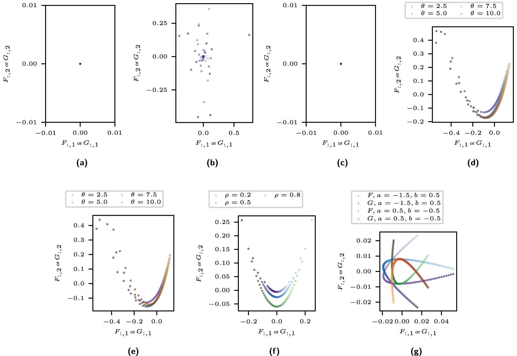
Row and column profiles for four copulas with various parameters, each with grid size
4.2 Profile plots illustrated with a data example
Using data from an engineering context, we apply the graphical dependence assessment to empirical data. Coblenz et al. [6] modeled the distribution of fuel drops that are generated by a fuel injector in a jet engine using vine copulas. The droplets are characterized by five variables
The published data of Coblenz et al. [6] are available in the rank-transformed copula domain, which we denote by
![Figure 13
Profile and checkerboard plots of the fuel injector spray characteristics in jet engines from Coblenz et al. [6]. The physical interpretations of the variables are drop size (
u
1
{u}_{1}
), x-position (
u
2
{u}_{2}
), y-position (
u
3
{u}_{3}
), x-velocity (
u
4
{u}_{4}
), and y-velocity (
u
5
{u}_{5}
): (a) row profiles for variables
u
2
{u}_{2}
and u
2, (b) column profiles for variables u
1 and u
2, (c) checkerboard plot for variables u
1 and u
2, (d) row profiles for variables u
1 and u
4, (e) column profiles for variables u
1 and u
4, (f) checkerboards plot for variables u
1 and u
4, (g) row profiles for variables u
2 and u
3, (h) column profiles for variables u
2 and u
3, (i) checkerboard plot for variables u
2 and u
3, (j) row profiles for variables u
2 and u
4. A profile at (0.60, 0.27) is out of scope, (k) column profiles for variables u
2 and u
4. A profile at (0.60, 0.27) is out of scope, (l) checkerboard copula plot for variables u
2 and u
4, (m) row profiles for variables u
3 and u
4, (n) column profiles for variables u
3 and u
4, and (o) checkerboard plot for variables u
3 and u
4.](/document/doi/10.1515/demo-2024-0006/asset/graphic/j_demo-2024-0006_fig_013.jpg)
Profile and checkerboard plots of the fuel injector spray characteristics in jet engines from Coblenz et al. [6]. The physical interpretations of the variables are drop size (
As profile points are obtained from empirical data, they deviate from their theoretical counterparts. To visualize statistical noise in the plots, we show the typical minimal and maximal values of profiles for an independence copula by a gray rectangle in the plots. The gray rectangles are obtained by sampling 5,252 realizations from an independence copula and computing their row and column profiles. The procedure is repeated 100 times. The rectangles cover 95% of the minimal and maximal point coordinates of the 100 samples in every dimension. Thus, if the profiles are outside the gray box, the underlying copula is unlikely to be the independence copula. This approach aligns with Greenacre [18], who advocates resampling methods, for example, bootstrapping, over using asymptotic results for profile values. Again, the darker the point’s color, the closer the conditional distribution’s conditioning variable is to one.
The profile plots for variables
Overall, the row and profile plots provide at least the same amount of information as the checkerboard plots, but they are more transparent and less cluttered than the checkerboard plots.
5 Conclusion
This article analyzes truncations of SVD and correspondence analysis of checkerboard copulas. Checkerboard copulas can be mapped to doubly stochastic matrices, making it straightforward to ensure copula properties for the approximations. We find that some common copulas, for example, comonotonicity-like, have high ranks and thus are poorly represented in the straightforward SVD and that truncations can have negative elements. To account for comonotonicity-like copulas with high ranks, we adapt a representation anchored with the comonotonicity copula and show its performance in examples. We compute the nearest valid doubly stochastic matrix to correct the truncations with negative entries. We analyze the representations of statistical characteristics of copulas, such as Kendall’s
Other approaches for reducing the comonoticity-like characteristics of the copula are possible, such as using rook copulas [7] and, for empirical data, sample-dependent grid sizes [22] or anchoring with respect to other copulas while varying the sample size [13]. They need more complex fitting of the parameters and components and might use different grid sizes. Thus, we leave the comparison of these methods for further research.
In this article, we do not expand on the empirical estimation of the model. It is well known that the empirical checkerboard copula converges to the theoretical checkerboard copula. Perturbation theory analyzes the effect of noise on the results of the SVD (for a concise overview, see, e.g., [46]). The singular vectors can suffer from large fluctuations for small noise; the singular values, however, are estimated more robustly. Thus, the visual analysis in Section 4 is less prone to noise than plotting the singular vectors directly.
Although the approach can be extended to larger dimensions, it is not straightforward. The concept of the checkerboard copula is viewed in a higher dimension, for example, in Carley and Taylor [5]. There is no direct analog of SVD in three and higher dimensions, but various approaches exist (see, for example, Kolda and Bader [26] for an introduction). Copula-specific methods for modeling high-dimensional data include vine copulas [3,14,23,36] and nested Archimedean copulas [20,42], where the copulas involved could be analyzed using the methods presented here.
Acknowledgements
We thank Johan Segers for his thoughtful and constructive discussions, as well as his insightful feedback, which have greatly enhanced the quality of this article. We extend our gratitude to the two anonymous reviewers whose valuable insights significantly improved this manuscript.
-
Funding information: We gratefully acknowledge the financial support provided by the Bischöfliche Studienförderung Cusanuswerk to JR and by the KIT publication fund for open access publishing.
-
Author contributions: Both authors have accepted responsibility for the entire content of this manuscript and consented to its submission to the journal and have reviewed all the results and approved the final version of the manuscript. OG: conceptualization, methodology, writing, supervision. JR: conceptualization, methodology, writing, software, simulation.
-
Conflict of interest: The authors have no conflicts of interest related to this publication.
Appendix A Calculations for the algorithms of Section 2.3
We consider the problem
with a symmetric matrix
The solution of
In the case of an asymmetric matrix
For
there exists a closed-form solution independent of the symmetry of
the solution of
A.1 Symmetric copula
The proof is analogous to Zass and Shashua [47] for symmetric
If
Then,
and
using
The result for
using
|
Algorithm 1: Algorithm to compute the nearest doubly stochastic matrix in terms of the Frobenius error following Zass and Shashua [47] for symmetric matrices
|
|
|---|---|
|
input Matrix
|
|
|
output: nearest doubly stochastic matrix
|
|
| 1 | Set
|
| 1 | Update
|
| 3 |
while
|
|
|
|
| 7 | end |
A.2 Asymmetric copula
For asymmetric
Instead, the solution of a Karush-Kuhn-Tucker equation system yields the solution for
with the Lagrange function and its derivative
yields the system
The solution of the Karush-Kuhn-Tucker equation system is the solution of the linear equation system
and
Additionally, Algorithm 1 includes a deflection component to account for the more general setting [17,47], as summarized in Algorithm 2.
|
Algorithm 2: Algorithm to compute the nearest doubly stochastic matrix in terms of the Frobenius error following Zass and Shashua [47] for asymmetric matrices
|
|
|---|---|
|
input: Matrix
|
|
|
output: Nearest doubly stochastic matrix
|
|
| 1 | Set
|
| 2 | Set
|
| 3 | Set
|
| 4 | repeat |
|
|
|
| 8 |
|
B Decomposition in terms of the Hellinger distance
The SVD and the algorithms of Section 2.3 yield minimal errors in terms of the Frobenius norm. The SVD is also the best low-rank approximation considering the spectral norm [34]. In statistics, the Hellinger distance is often used to assess the proximity of densities (see [1,32], for two recent contributions). In this section, we analyze Hellinger distance-based decompositions for two different versions of the Hellinger distance for matrices, as, to our knowledge, there is no agreed definition in the matrix case yet. For a matrix square root-based Hellinger distance, the decomposition generalizes from the Frobenius case, while it is of a different and more complicated structure for an elementwise square root Hellinger distance.
For discrete probability distributions
For matrices, there are different notions of the Hellinger distance in the literature. We consider a formulation based on the matrix square root first [4] and then turn to an elementwise square root method [39].
Bhatia et al. [4] started from the decomposition of the Hellinger distance for densities into an arithmetic and geometric mean. As the geometric mean for matrices can be interpreted in various ways, different notions of the distance can be obtained. We use their most straightforward generalization yielding the Hellinger distance for positive semidefinite, and thus, symmetric, matrices
Thereby,
Lemma 3
The low-rank approximation problem of a positive definite matrix A yields the same eigenvectors and eigenvalues for the Frobenius and the Hellinger distance.
Proof
Let
and
as the matrix square root is unique and
Thus, the minimizing argument,
exists with eigenvector matrix
The eigenvectors of
Thus, the minimizing argument of
and equal to the minimizing argument of
This definition of the Hellinger distance obtains the same decomposition as with the Frobenius distance. The coefficient
Rao [39] and Cuadras and Cuadras [11] defined the Hellinger distance in terms of an elementwise square root, thus considering only matrices with non-negative elements. Let
Truncations
All in all, the elementwise Hellinger decomposition is not as straightforward as the Frobenius decomposition, as the squared decomposition does not keep the rank of the truncation, and the attached optimization problems obtain more complex. Through the elementwise square root, the influence of peaks in the checkerboard copula on the objective function is reduced compared to the Frobenius case. It is a modeling choice, whether this is desired or not. Rao [39] and Cuadras and Cuadras [11] pointed out that elementwise Hellinger-based decomposition’s main advantage is the independence from the row and column marginals. However, the marginals are constant in the checkerboard copula setting; thus, the correspondence analysis does not depend on them. Thus, we do not expand on the Hellinger decompositions in the main part of this article.
C Computations for Spearman’s
ρ
and Kendall’s
τ
in Section 2.4
As in Section 2.4,
Similarly, follows for the MAR decomposition,
where
The respective computations for Kendall’s
and for the MAR analogously.
D Further figures for Section 4.2
![Figure A1
Remaining profile and checkerboard plots of the fuel injector spray characteristics in jet engines from Coblenz et al. [6] from Section 4.2. The other dimension combinations are shown in Figure 13. The physical interpretations of the variables are drop size (
u
1
{u}_{1}
), x-position (
u
2
{u}_{2}
), y-position (
u
3
{u}_{3}
), x-velocity (
u
4
{u}_{4}
), and y-velocity (
u
5
{u}_{5}
). For the variable pairs (
u
1
{u}_{1}
,
u
5
{u}_{5}
) and (
u
2
{u}_{2}
,
u
5
{u}_{5}
), no deviation from independence is discernible. A weak hump-shape can be observed for variables
u
1
{u}_{1}
and
u
3
{u}_{3}
. Again, the course of column profiles is reversed in the middle of the profiles. The plots show a Gaussian-like behavior for variables
u
3
{u}_{3}
and
u
5
{u}_{5}
. The profile plots for variables
u
4
{u}_{4}
and
u
5
{u}_{5}
show a weak deviation from independence for the profiles near
u
4
=
1
{u}_{4}=1
and extreme values of
u
5
{u}_{5}
: (a) row profiles for variables
u
1
{u}_{1}
and
u
3
{u}_{3}
, (b) column profiles for variables
u
1
{u}_{1}
and
u
3
{u}_{3}
, (c) checkerboard plot for variables
u
1
{u}_{1}
and
u
3
{u}_{3}
, (d) row profiles for variables
u
1
{u}_{1}
and
u
5
{u}_{5}
, (e) column profiles for variables
u
1
{u}_{1}
and
u
5
{u}_{5}
, (f) checkerboard plot for variables
u
1
{u}_{1}
and
u
5
{u}_{5}
, (g) row profiles for variables
u
2
{u}_{2}
and
u
5
{u}_{5}
, (h) column profiles for variables
u
2
{u}_{2}
and
u
5
{u}_{5}
, (i) checkerboard plot for variables
u
2
{u}_{2}
and
u
5
{u}_{5}
, (j) row profiles for variables
u
3
{u}_{3}
and
u
5
{u}_{5}
, (k) column profiles for variables
u
3
{u}_{3}
and
u
5
{u}_{5}
, (l) checkerboard plot for variables
u
3
{u}_{3}
and
u
5
{u}_{5}
, (m) Row profiles for variables
u
4
{u}_{4}
and
u
5
{u}_{5}
, (n) column profiles for variables
u
4
{u}_{4}
and
u
5
{u}_{5}
, and (o) checkerboard plot for variables
u
4
{u}_{4}
and
u
5
{u}_{5}
.](/document/doi/10.1515/demo-2024-0006/asset/graphic/j_demo-2024-0006_fig_014.jpg)
Remaining profile and checkerboard plots of the fuel injector spray characteristics in jet engines from Coblenz et al. [6] from Section 4.2. The other dimension combinations are shown in Figure 13. The physical interpretations of the variables are drop size (
References
[1] Aya-Moreno, C., Geenens, G., Penev, S. (2018). Shape-preserving wavelet-based multivariate density estimation. Journal of Multivariate Analysis, 168, 30–47, DOI: https://doi.org/10.1016/j.jmva.2018.07.002. 10.1016/j.jmva.2018.07.002Search in Google Scholar
[2] Bakam, Y. I. N., Pommeret, D. (2022). K-Sample test for equality of Copulas. Search in Google Scholar
[3] Bedford, T., Cooke, R. M. (2002). Vines-a new graphical model for dependent random variables. The Annals of Statistics, 30(4), 1031–1068, DOI: https://doi.org/10.1214/aos/1031689016. 10.1214/aos/1031689016Search in Google Scholar
[4] Bhatia, R., Gaubert, S., Jain, T. (2019). Matrix versions of the Hellinger distance. Letters in Mathematical Physics, 109(8), 1777–1804. 10.1007/s11005-019-01156-0Search in Google Scholar
[5] Carley, H., Taylor, M. D. (2002). A new proof of Sklar’s theorem. In: Distributions with given marginals and statistical modelling (pp. 29–34), Netherlands: Springer. 10.1007/978-94-017-0061-0_4Search in Google Scholar
[6] Coblenz, M., Holz, S., Bauer, H.-J., Grothe, O., Koch, R. (2020). Modelling fuel injector spray characteristics in jet engines by using vine copulas. Journal of the Royal Statistical Society Series C: Applied Statistics, 69(4), 863–886. 10.1111/rssc.12421Search in Google Scholar
[7] Cottin, C., Pfeifer, D. (2014). From Bernstein polynomials to Bernstein copulas. Journal of Applied Functional Analysis, 9, 277–288. Search in Google Scholar
[8] Cuadras, C. M. (2015). Contributions to the diagonal expansion of a bivariate copula with continuous extensions. Journal of Multivariate Analysis, 139, 28–44. 10.1016/j.jmva.2015.02.015Search in Google Scholar
[9] Cuadras, C. M. (2002). Correspondence analysis and diagonal expansions in terms of distribution functions. Journal of Statistical Planning and Inference, 103(1–2), 137–150. 10.1016/S0378-3758(01)00216-6Search in Google Scholar
[10] Cuadras, C. M., Augé, J. (1981). A continuous general multivariate distribution and its properties. Communications in Statistics - Theory and Methods, 10(4), 339–353. 10.1080/03610928108828042Search in Google Scholar
[11] Cuadras, C. M., Cuadras, D. (2006). A parametric approach to correspondence analysis. Linear Algebra and its Applications, 417(1), 64–74. 10.1016/j.laa.2005.10.029Search in Google Scholar
[12] Cuadras, C. M., Díaz, W. (2012). Another generalization of the bivariate FGM distribution with two-dimensional extensions. Acta et Commentationes Universitatis Tartuensis de Mathematica 16(1), 3–12. 10.12697/ACUTM.2012.16.01Search in Google Scholar
[13] Cuberos, A., Masiello, E., Maume-Deschamps, V. (2020). Copulas checker-type approximations: Application to quantiles estimation of sums of dependent random variables. Communications in Statistics - Theory and Methods, 49(12), 3044–3062. 10.1080/03610926.2019.1586936Search in Google Scholar
[14] Czado, C. (2019). Analyzing Dependent Data with Vine Copulas, vol. 222. Cham: Springer International Publishing. 10.1007/978-3-030-13785-4Search in Google Scholar
[15] Durante, F., Sempi, C. (2015). Principles of Copula Theory. New York: Chapman and Hall/CRC.10.1201/b18674Search in Google Scholar
[16] Durrleman, V., Nikeghbali, A., Roncalli, T. (2000). Copulas Approximation and New Families. DOI: https://doi.org/10.2139/ssrn.1032547.10.2139/ssrn.1032547Search in Google Scholar
[17] Dykstra, R. L. (1983). An algorithm for restricted least squares regression. Journal of the American Statistical Association, 78(384), 837–842. 10.1080/01621459.1983.10477029Search in Google Scholar
[18] Greenacre, M. J. (1984). Theory and applications of correspondence analysis. London: Academic Press. Search in Google Scholar
[19] Hill, M. O. (1974). Correspondence analysis: A neglected multivariate method. Applied Statistics, 23(3), 340–354. 10.2307/2347127Search in Google Scholar
[20] Hofert, M., Hofert, M., Mächler, M. (2011). Nested Archimedean copulas meet R: The nacopula package. Journal of Statistical Software, 39(9), 1–20. 10.18637/jss.v039.i09Search in Google Scholar
[21] Horn, R. A., Johnson, C. R. (2012). Matrix Analysis. 2nd edition, Cambridge; New York: Cambridge University Press. 10.1017/CBO9781139020411Search in Google Scholar
[22] Janssen, P., Swanepoel, J., Veraverbeke, N. (2012). Large sample behavior of the Bernstein copula estimator. Journal of Statistical Planning and Inference, 142(5), 1189–1197, DOI: https://doi.org/10.1016/j.jspi.2011.11.020. 10.1016/j.jspi.2011.11.020Search in Google Scholar
[23] Joe, H. (1996). Families of m-variate distributions with given margins and m(m‒1)⁄2 bivariate dependence parameters. Lecture Notes-Monograph Series, 28, 120–141. 10.1214/lnms/1215452614Search in Google Scholar
[24] Kazmierczak, J.-B. (1978). Migrations interurbaines dans la banlieue sud de paris. Cahiers de laanalyse des données, 3(2), 203–218. Search in Google Scholar
[25] Klaassen, C. A. J., Wellner, J. A. (1997). Efficient estimation in the bivariate normal copula model: normal margins are least favourable. Bernoulli, 3(1), 55, DOI: https://doi.org/10.2307/3318652. 10.2307/3318652Search in Google Scholar
[26] Kolda, T. G., Bader, B. W. (2009). Tensor decompositions and applications. SIAM Review, 51(3), 455–500. 10.1137/07070111XSearch in Google Scholar
[27] Kolesárová, A., Mesiar, R., Mordelová, J., Sempi, C. (2006). Discrete copulas. IEEE Transactions on Fuzzy Systems, 14(5), 698–705. 10.1109/TFUZZ.2006.880003Search in Google Scholar
[28] Lancaster, H. O. (1957). Some properties of the bivariate normal distribution considered in the form of a contingency table. Biometrika, 44(1–2), 289–292, DOI: https://doi.org/10.1093/biomet/44.1-2.289.10.1093/biomet/44.1-2.289Search in Google Scholar
[29] Li, X., Mikusiński, P., Sherwood, H., Taylor, M. D. (1997). On approximation of copulas. In Beneš, V., Štěpán, J., editors, Distributions with given Marginals and Moment Problems (pp. 107–116). Netherlands: Springer. 10.1007/978-94-011-5532-8_13Search in Google Scholar
[30] Masuhr, A., Trede, M. (2020). Bayesian estimation of generalized partition of unity copulas. Dependence Modeling, 8(1), 119–131, DOI: https://doi.org/10.1515/demo-2020-0007. 10.1515/demo-2020-0007Search in Google Scholar
[31] Mayor, G., Suner, J., Torrens, J. (2005). Copula-like operations on finite settings. IEEE Transactions on Fuzzy Systems, 13(4), 468–477, DOI: https://doi.org/10.1109/TFUZZ.2004.840129. 10.1109/TFUZZ.2004.840129Search in Google Scholar
[32] Meier, C., Kirch, C., Meyer, R. (2018). Bayesian nonparametric analysis of multivariate time series: a matrix gamma process approach. Journal of Multivariate Analysis, 175, 104560, DOI: https://doi.org/10.1016/j.jmva.2019.104560. 10.1016/j.jmva.2019.104560Search in Google Scholar
[33] Mesiar, R., Najjari, V. (2014). New families of symmetric/asymmetric copulas. Fuzzy Sets and Systems, 252, 99–110. 10.1016/j.fss.2013.12.015Search in Google Scholar
[34] Mirsky, L. (1960). Symmetric Gauge functions and unitarily invariant norms. The Quarterly Journal of Mathematics, 11(1), 50–59. 10.1093/qmath/11.1.50Search in Google Scholar
[35] Nelsen, R. B. (2006). An Introduction to Copulas. Springer Series in Statistics. New York, NY: Springer New York. Search in Google Scholar
[36] Panagiotelis, A., Czado, C., Joe, H., Stöber, J. (2017). Model selection for discrete regular vine copulas. Computational Statistics & Data Analysis, 106, 138–152. 10.1016/j.csda.2016.09.007Search in Google Scholar
[37] Perfect, H., Mirsky, L. (1965). Spectral properties of doubly-stochastic matrices. Monatshefte für Mathematik, 69(1), 35–57, DOI: https://doi.org/10.1007/BF01313442. 10.1007/BF01313442Search in Google Scholar
[38] Pfeifer, D., Tsatedem, H. A., Mändle, A., Girschig, C. (2016). New copulas based on general partitions-of-unity and their applications to risk management. Dependence Modeling, 4(1), 000010151520160006, DOI: https://doi.org/10.1515/demo2016-0006. 10.1515/demo-2016-0006Search in Google Scholar
[39] Rao, C. R. (1995). A review of canonical coordinates and an alternative to correspondence analysis using Hellinger distance. Qüestiió, 19(1-2-3), 23–63. Search in Google Scholar
[40] Rodríguez-Lallena, J. (2004). A new class of bivariate copulas. Statistics & Probability Letters, 66(3), 315–325. 10.1016/j.spl.2003.09.010Search in Google Scholar
[41] Rontsis, N., Goulart, P. (2020). Optimal approximation of doubly stochastic matrices. In: Chiappa, S., Calandra, R., editors, Proceedings of the Twenty Third International Conference on Artificial Intelligence and Statistics, volume 108 of Proceedings of Machine Learning Research (pp. 3589–3598). Search in Google Scholar
[42] Savu, C., Trede, M. (2010). Hierarchies of Archimedean copulas. Quantitative Finance, 10(3), 295–304. 10.1080/14697680902821733Search in Google Scholar
[43] Savu, C., Trede, M. (2008). Goodness-of-fit tests for parametric families of Archimedean copulas. Quantitative Finance, 8(2), 109–116, DOI: https://doi.org/10.1080/14697680701207639. 10.1080/14697680701207639Search in Google Scholar
[44] Schmid, F., Schmidt, R., Blumentritt, T., Gaißer, S., Ruppert, M. (2010). Copula-based measures of multivariate association. In Jaworski, P., Durante, F., Härdle, W. K., Rychlik, T., editors, Copula Theory and Its Applications (vol. 198, pp. 209–236). Springer Berlin Heidelberg. 10.1007/978-3-642-12465-5_10Search in Google Scholar
[45] Sklar, A. (1959). Fonctions de répartition à n dimensions et leurs marges. Publications de L’Institut de Statistique de L’Université de Paris, 8, 229–231. Search in Google Scholar
[46] Stewart, G. W. (1991). Perturbation theory for the singular value decomposition. In: Vaccaro, R. J., editor, and University of Rhode Island, SVD and Signal Processing, II: Algorithms, Analysis, and Applications, Amsterdam; New York: New York, N.Y., U.S.A: Elsevier; Distributors for the U.S.A. and Canada, Elsevier Science Pub. Co., (pp. 99–109). Search in Google Scholar
[47] Zass, R., Shashua, A. (2007). Doubly stochastic normalization for spectral clustering. In: Schölkopf, B., Platt, J., Hofmann, T., editors, Advances in Neural Information Processing Systems (vol. 19, pp. 1569–1576). The MIT Press. 10.7551/mitpress/7503.003.0201Search in Google Scholar
© 2024 the author(s), published by De Gruyter
This work is licensed under the Creative Commons Attribution 4.0 International License.
Articles in the same Issue
- Research Articles
- Sharp bounds on the survival function of exchangeable min-stable multivariate exponential sequences
- Invariance properties of limiting point processes and applications to clusters of extremes
- Assessing copula models for mixed continuous-ordinal variables
- Using sums-of-squares to prove Gaussian product inequalities
- On the construction of stationary processes and random fields
- Decomposition and graphical correspondence analysis of checkerboard copulas
- Special Issue on 40th Linz Seminar
- Special Issue: 40th Linz Seminar on Fuzzy Set Theory. Copulas – Theory and Applications
- Geometry of generators of triangular norms and copulas
- Dependence properties of bivariate copula families
- Median and quantile conditional copulas
- On comprehensive families of copulas involving the three basic copulas and transformations thereof