A nonparametric test for comparing survival functions based on restricted distance correlation

1 Introduction

To evaluate the treatment effect for survival data, we often need to compare the survival functions of the treatment and control groups. The most popular approach to comparing survival functions is the log-rank test, and it is well known that under proportional hazards, the log-rank test is optimal and equivalent to the score test in Cox regression model. When the proportional hazard assumption is moderately or severely violated, however, the log-rank test might be suboptimal. In many clinical studies, especially cancer immunotherapy trials [1,19,24], the violation of proportional hazards assumption is often encountered, and different patterns of non-proportional hazards are frequently observed, e.g., delayed treatment effect, diminishing effect, and crossing survival curves, making the traditional log-rank test underpowered. One way to address this challenge is using the weighted log-rank test, and a popular weight function is the Fleming-Harrington (FH) weight with parameters ρ and γ ,

where S n ( t − ) is the estimated survival function immediately prior to time t . The choice of ρ and γ can handle different types of treatment effect. For instance, w FH ( t ; ρ > 0 , γ = 0 ) is good for early separation, w FH ( t ; ρ = 0 , γ > 0 ) for late separation, and w PH ( t ; ρ > 0 , γ > 0 ) for middle separation. However, none of these tests is good for all situations, and a prior misspecification of the weight function may decrease the power of the test. Motivated by previous studies [13,26], a cross-industry working group proposed a maxCombo test by taking the maximum of multiple FH-weighted log-rank statistics [14]. One such combination is

where Z FH ( ρ , γ ) stands for the Z -statistic of the weighted log-rank test with w FH ( t ; ρ , γ ) , and it can be shown that [ Z FH ( 0 , 0 ) , Z FH ( 0 , 1 ) , Z FH ( 1 , 0 ) , Z FH ( 1 , 1 ) ] T are asymptotically joint normal. Using simulated data, Lin et al. [14] showed that the maxCombo test has good statistical power under proportional hazard and different patterns of non-proportional hazards, thus it can be used as an omnibus test for a broad class of alternative hypotheses. A robust version of maxCombo based on weights [ ( 0 , 0 ) , ( 0 , 1 ∕ 2 ) , ( 1 ∕ 2 , 0 ) , ( 1 ∕ 2 , 1 ∕ 2 ) ] is suggested by Roychoudhury et al. [18].

In addition to the maxCombo test, there are many other omnibus tests developed for survival data. To name a few, Fleming et al. generalized the Kolmogorov-Smirnov (KS) test for arbitrarily right-censored data [8]. Koziol et al. and Schumacher modified the Crámer-von Mises (CVM) test under the assumption of randomly censoring [12,20]. All these KS- or CVM-based methods can be viewed as a weighted L p distance ( p = 2 for CVM and p = ∞ for KS) between two Kaplan-Meier (KM) curves or Nelson-Aalen curves. With the intent of addressing crossing survival curves, Qiu and Sheng proposed a two-stage procedure, where the log-rank test is used in the first stage and a particular weighted log-rank test is used in the second stage [16]. The weight function in stage two is chosen to change signs before and after a potential crossing point, boosting its power for crossing survival curves. Recently, Ditzhaus et al. proposed a permutation test based on the Nelson-Aalen-type integrals without any restrictive model assumption [3]. Fernández et al. introduced a general nonparametric independence test between right-censored survival times and covariates based on the supremum of a potentially infinite collection of weight-indexed log-rank tests, with weight functions belonging to a reproducing kernel Hilbert space (RKHS) of functions [7].

In this study, we shall develop a new omnibus test for comparing survival functions. The test statistic is based on a restricted version of distance correlation and related to the unweighted L 2 distance between two survival functions. Motivated by Edelmann et al. [5] and Zhang et al. [28], a permutation procedure based on the product-limit estimator is used for implementing our method. Simulation studies show that the new test performs well under different sample sizes and survival models.

The remainder of this study is structured as follows: Section 2 introduces the notion of restricted distance correlation, and proposes a consistent estimator. Section 3 evaluates the performance of the new and existing tests under different non-proportional hazards settings. Section 4 discusses the method with some future perspectives.

2 Restricted distance correlation test

In this section, we introduce the restricted distance correlation test for survival data and establish its statistical consistency. We begin with the notations. For subject i ∈ { 1 , … , n } , let T i denote the survival time, X i the group index (0 for the control arm, 1 for the treatment arm), π = P ( X i = 1 ) , and C i the censoring time due to administrative censoring or patient dropout. The observed event or censoring time is defined as U i = min { T i , C i } , with event indicator δ i = I { T i ≤ C i } . Let f 0 ( t ) , f 1 ( t ) , F 0 ( t ) , F 1 ( t ) , S 0 ( t ) , S 1 ( t ) be the probability density functions (p.d.f.), cumulative distribution functions (c.d.f.), and survival functions of T in two arms, i.e., f 0 ( t ) = f ( t ∣ X i = 0 ) , and f 1 ( t ) = f ( t ∣ X i = 1 ) , F 0 ( t ) = F ( t ∣ X i = 0 ) , F 1 ( t ) = F ( t ∣ X i = 1 ) , S 0 ( t ) = 1 − F ( t ∣ X i = 0 ) , and S 1 ( t ) = 1 − F ( t ∣ X i = 1 ) . Let G ( t ) be the c.d.f. of C i for both arms and τ be the study duration ( max i C i ≤ τ ). The null and alternative hypotheses can be formulated as follows:

It is noteworthy that testing (1) amounts to testing the independence between the survival time T and group index X , where T is continuous and X is binary. Herein, we consider the distance correlation test by Székely et al. [23]. The distance covariance between two random vectors X and Y is defined as the square root of

where c d x = π ( 1 + d x ) ∕ 2 Γ { ( 1 + d x ) ∕ 2 } and c d y = π ( 1 + d y ) ∕ 2 Γ { ( 1 + d y ) ∕ 2 } , ‖ z ‖ d z denotes the Euclidean norm of z ∈ R d z , and ‖ ϕ ‖ 2 = ϕ ϕ ¯ for a complex-valued function ϕ and its conjugate ϕ ¯ [15,23]. Similar to Pearson’s correlation coefficient, the distance correlation is defined as follows:

One remarkable property of distance correlation is that it is 0 if and only if X and Y are statistically independent, indicating that the distance correlation can detect any form of association. Székely et al. [23] also provided the following alternative definition of dCov 2 ( X , Y ) :

where ( X 1 , Y 1 ) , ( X 2 , Y 2 ) , and ( X 3 , Y 3 ) stand for three independent copies of ( X , Y ) .

As a special case of (3), in the following, we give the explicit formula of squared distance correlation between the survival time T and group index X (the detailed proof is provided in Appendix A.1):

Noteworthily, the squared distance covariance between X and T (see equation (A1) in A.1) is equivalent to the energy distance between T ∣ X = 0 and T ∣ X = 1 . In fact, up to a constant multiple, equation (A1) is also equivalent to Crámer’s distance [2] between T ∣ X = 0 and T ∣ X = 1 . Crámer’s distance can be viewed as a special case of energy distance when both variables are univariate. However, as Rizzo and Székely [17] pointed out, the equivalence of energy distance with Crámer’s distance cannot extend to higher dimensions, because while energy distance is rotation invariant, Crámer’s distance is not.

For clinical trials with survival endpoints, an administrative censoring is often applied at the end of the study period so that no event can be observed after time τ , i.e., max i C i ≤ τ . Similar to the restricted mean survival time (RMST), we consider a restricted version of distance correlation on [ 0 , τ ] for hypothesis testing

The null and alternative hypotheses based on the restricted distance correlation can be formulated as:

Under the restriction of total study duration, the null hypothesis in (6) can be interpreted as the independence between T and X conditioning on 0 ≤ T ≤ τ , i.e., T ⊥ X ∣ 0 ≤ T ≤ τ . With a sufficient study duration τ , e.g., max { S 0 ( τ ) , S 1 ( τ ) } is small, (6) can be used as a proxy of (1), but results should not be over-interpreted for relatively short τ .

Assuming independent censoring, i.e., T ⊥ C , let S 1 n ( t ) and S 0 n ( t ) be some consistent estimators of S 1 ( t ) and S 0 ( t ) , such as the product-limit estimator or the piecewise exponential estimator [11]. For simplicity, we consider the following product-limit estimate:

Theorem 1 establishes the statistical consistency of (7), under mild regularity conditions (proof is given in Appendix A.2).

In general, the null distribution of distance correlation is impractical to derive as it depends on the underlying distributions of X and Y ; therefore, we suggest a permutation procedure to evaluate significance. One may first calculate the test statistic dCor n 2 ( T , X ; τ ) for the observed data, then for each b = 1 , … , B , calculate the distance correlation dCor b 2 ( T , X ; τ ) based on the random permutation of group indices { X i , i = 1 , … , n } . The permutation p -value can be computed as:

Though the formula for dCor n 2 ( T , X ; τ ) seems unwieldy, for the purposes of constructing a permutation test, only the numerator is relevant. The numerator is essentially a L 2 distance between S 1 n ( t ) and S 0 n ( t ) , which is closely related to the CVM criterion. The CVM statistic is

which is a L 2 distance between two estimated survival functions with weight π f 1 n ( t ) + ( 1 − π ) f 0 n ( t ) . The CVM statistic assigns more weight on time points with higher event rates; thus, for concave-up survival functions, it tends to better detect early separation than late separation. In contrast, our distance correlation statistic is an unweighted L 2 distance, targeting the difference between two survival curves for the entire study period.

3 Two extensions of the proposed test

A limitation of the restricted distance correlation test is that it is only for two-sided alternatives, therefore not suitable for superiority tests that can be formulated as:

To this end, we also suggest a directional test by incorporating the sign information in L 2 distance. The directional statistic for permutation test can be written as:

where sgn ( ) is the sign function, i.e., sgn ( x ) = 1 if x ≥ 0 and sgn ( x ) = − 1 if x < 0 . Similar to (8), the permutation p -value can be computed as:

Second, as suggested by the reviewers, we extend the proposed distance correlation test to the Gaussian kernel, which can be equivalently used in the distance correlation formulation [6,10,22]. We derived the distance covariance between X and T based on the Gaussian kernel with bandwidth parameter σ 2 (see Appendix A.3 for details). For illustrative purposes, we present the formula for π = 1 ∕ 2 as follows:

where

The expected distances D 00 , D 11 , and D 01 can be estimated by replacing the survival functions S 0 ( t ) and S 1 ( t ) with the KM estimates S 0 n ( t ) and S 1 n ( t ) . A permutation test similar to equation (12) can then be performed based on D 00 + D 11 − 2 D 01 . In general, the tuning parameter σ 2 in the Gaussian kernel affects the testing power, and the effect depends on the data. Therefore, a data-driven approach should be used for selecting σ 2 . Our simulation studies have shown that the median survival of the pooled data (two arms) performs well under different settings; therefore, we suggest using it for σ 2 .

4 Simulation study

In this section, we conduct simulation studies to evaluate the performance of the restricted distance correlation test under different settings. In particular, we investigate the empirical statistical power and type I error rate under both two-sided and one-sided settings.

4.1 Two-sided alternatives

We compare the distance correlation tests (based on Euclidean distance and Gaussian kernel, respectively) with five existing tests, namely, (1) the robust maxCombo test, (2) two-stage test, (3) KS test, (4) CVM test, and (5) log-rank test. The log-rank test is used as a gold standard for proportional hazard, and it was implemented using R function survdiff in the survival package. The robust maxCombo test was implemented using the logrank.maxtest function in the nph package. The two-stage test by Qiu and Sheng [16] was implemented by the two-stage function in the TSHRC package. For KS, CVM, and our restricted distance correlation tests, p -values were computed based on 2,000 random permutations. The CVM test is based on equation (9), and the KS test is based on the following statistic:

(13) KS n ( τ ) = max 0 ≤ t ≤ τ ∣ S 1 n ( t ) − S 0 n ( t ) ∣ .

In the simulation, we set π = 1 ∕ 2 , and n = 60 , 100 , 150 , and 200 (total sample size for two arms). For all subjects, the loss to follow-up time (in months) is assumed to be exponential with rate parameter 0.005, corresponding to a 5.8% annual dropout rate and 26% five-year dropout rate. Moreover, we assume that the accrual time follows a uniform distribution over 3 years. Four alternatives, namely, a proportional hazards setting (A) and three non-proportional hazards settings (B: delayed treatment effect, C: crossing survival curves, D: diminishing effect), were constructed using exponential mixture models (similar curves can be also constructed by other flexible models such as generalized Weibull models or piecewise exponential models). The survival function of a two-component exponential mixture model is as follows:

(14) S j ( t ; γ j , λ j 1 , λ j 2 ) = γ j exp ( − λ j 1 t ) + ( 1 − γ j ) exp ( − λ j 2 t ) , j ∈ { 0 , 1 } ,

where γ j and 1 − γ j represent the proportions of two components in arm j , and λ j 1 and λ j 2 are the corresponding rate parameters. The parameters of each simulation setting are listed in the following, and the survival curves are sketched in Figure 1.

1. Proportional hazards: γ 0 = γ 1 = 1 , λ 01 = log ( 2 ) ∕ 15 , λ 11 = log ( 2 ) ∕ 22.5 .

2. Delayed treatment effect: γ 0 = γ 1 = 0.5 , λ 01 = log ( 2 ) ∕ 20 , λ 02 = log ( 2 ) ∕ 10 , λ 11 = log ( 2 ) ∕ 70 , λ 12 = log ( 2 ) ∕ 7 .

3. Crossing survival curves: γ 0 = γ 1 = 0.2 , λ 01 = log ( 2 ) ∕ 20 , λ 02 = log ( 2 ) ∕ 20 , λ 11 = log ( 2 ) ∕ 1 , λ 12 = log ( 2 ) ∕ 40 .

4. Diminishing effect: γ 0 = γ 1 = 0.1 , λ 01 = log ( 2 ) ∕ 20 , λ 02 = log ( 2 ) ∕ 3 , λ 11 = log ( 2 ) ∕ 20 , λ 12 = log ( 2 ) ∕ 5 .

Figure 1

Survival curves in the simulation study (a: proportional hazards, b: delayed treatment effect, c: crossing survival curves, and d: diminishing effect), where red represents the control arm and blue represents the treatment arm.

Figure 2 summarizes the empirical power over 5,000 simulations at the significance level of 0.05. The two distance correlation metrics perform comparably across all settings, with the Gaussian kernel performing slightly better than Euclidean distance. For example, in the proportional hazard setting with a sample size of 100, the test based on Euclidean distance achieves a power of 39%, while the test based on the Gaussian kernel achieves a power of 41%. In the proportional hazards setting, the log-rank test has the highest power. The distance correlation tests are the best among all omnibus tests, and when n = 200 , our tests achieve similar statistical power to the log-rank test. For Setting B, the distance correlation tests have the highest power among all methods. The maxCombo, log-rank, and two-stage tests also have good performance especially for relatively large sample sizes. It is noteworthy that the CVM test has low power in this delayed treatment effect setting, because it assigns more weight on the early stage and less weight on the late stage. For crossing survival curves (Setting C), the most powerful test is the two-stage test by Qiu and Sheng [16]. The two-stage procedure is particularly designed for crossing survival curves; thus, it is sensitive to this pattern. Our new tests have the second highest power in this setting, close to the robust maxCombo test. For the diminishing effect setting (Setting D), where the separation occurs at the early and middle stage, CVM provides the best power. The KS and distance correlation tests have slightly lower power than CVM. Overall, our distance correlation tests have satisfactory power for different settings; thus, it can be an competitive alternative to the existing ones.

Figure 2

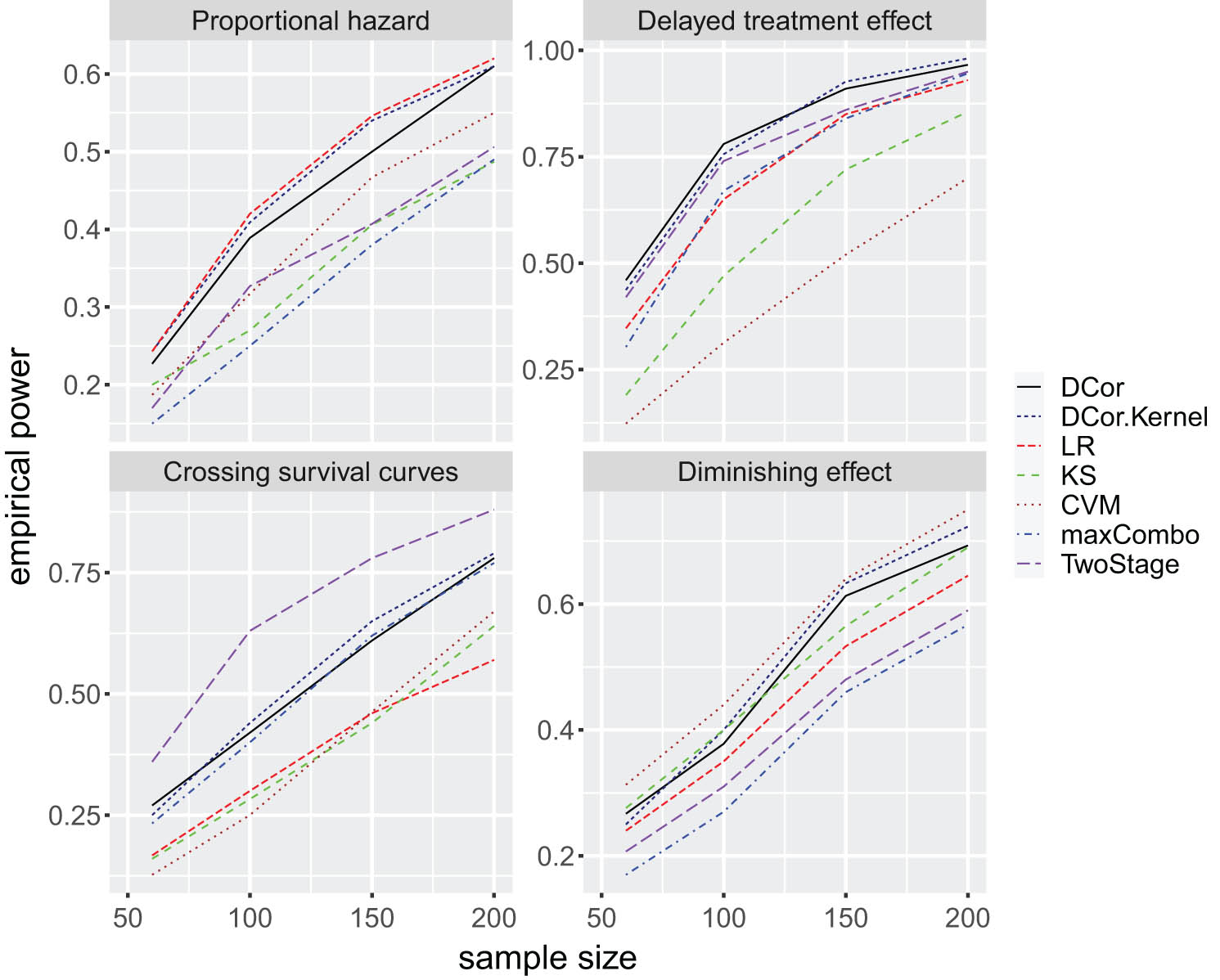
Empirical power over 5,000 simulations for two-sided alternatives.

We also investigated the type I error rate control under different sample sizes. Figure 3 presents the type I error rate over 10,000 simulations (under the null model γ 0 = γ 1 = 1 , λ 01 = λ 11 = log ( 2 ) ∕ 15 ). All the tests control the type I error rate. The three permutation based tests, namely KS, CVM, and restricted distance correlation tests, have type I error rates close to the nominal level of 0.05. The log-rank test and maxCombo test based on weighted log-rank statistics are slightly conservative when sample size is small, e.g., n = 60 .

Figure 3

Type I error rate over 10,000 simulations for two-sided alternatives.

4.2 One-sided alternatives

For one-sided alternatives, we compare our directional distance correlation test (equations (11) and (12)) with (1) log-rank test, (2) RMST test, and (3) the robust maxCombo, under the same simulation settings as detailed in Section 3.1. The two-stage, CVM, and KS tests are excluded in the analysis because they are not suitable for one-sided alternatives. Figure 4 displays the empirical power over 5,000 simulations at the significance level of 0.05. Same as what we observed in the two-sided case, in the proportional hazards setting, the log-rank test has the highest statistical power. Our distance correlation test has similar power to RMST, both higher than maxCombo. In the delayed treatment effect setting, the RMST and distance correlation tests substantially outperform the log-rank and maxCombo tests. Specifically, the maxCombo test is the most powerful test for detecting differences between crossing survival curves (Setting C). In the diminishing effect setting, the distance correlation test has the greatest power, slightly higher than the log-rank test. Overall, our distance correlation test have satisfactory power across different settings. Figure 5 summarizes the empirical sizes of the four tests, where it can be seen that all four tests control the type I error rate, and three RMST tests are slightly conservative.

Figure 4

Empirical power over 5,000 simulations for one-sided alternatives.

Figure 5

Type I error rate over 10,000 simulations for one-sided alternatives.

5 Discussion and conclusions

In recent clinical studies, especially in cancer immunotherapy studies, the violation of the proportional hazards assumption is often encountered; thus, the traditional log-rank test may not be optimal. In this work, we propose a simple and versatile test to compare survival curves under non-proportional hazards. The test statistic is derived from a restricted version of the widely used distance correlation metric, which is essentially the L 2 distance between the KM curves of two treatment groups. Our simulation studies show that the new test is powerful under both proportional hazards and different types of non-proportional hazards.

One major limitation of the proposed test is the lack of an analytical formula for computing p -values. Therefore, it would be of great interest to investigate the asymptotic behavior of the restricted distance correlation theoretically. While the sampling distribution of the distance correlation is generally impractical to derive, Shen et al. [21] derived a chi-square distribution that well approximates and dominates the limiting null distribution in the upper tail. They showed that under the bias-corrected estimate of the distance correlation, the chi-square test exhibits similar testing power to the standard permutation test. However, the existence of censored samples in survival data makes it difficult to obtain the bias-corrected estimate. Therefore, directly applying the chi-squared approximation based on the KM estimates may result in low power. Figure 6 presents a comparison of the power of the permutation test and Shen et al.’s chi-squared approximation. As can be seen, the chi-squared test can be very conservative, especially when the sample size is relatively small (e.g., n = 60 ). To circumvent this problem, we need to find a new estimate or approximating distribution function to calculate an upper bound of the p -value. We leave this as a topic for future research.

Figure 6

Power comparison for the permutation test and chi-squared test.

Another practical limitation is the assumption of independent censoring, meaning that the censoring time is independent of both groups and survival time. When the censoring depends on groups, the permutation test may have an inflated type I error rate; even, the survival curves are equal. To illustrate this, we performed simulations (Figure 7) and found that the type I error rate inflation is non-negligible when there is a substantial difference in the censoring rate between two arms. Therefore, it is important to check whether the two arms have similar censoring distributions before using a distance correlation test. Possible approaches for estimating censoring distributions or censoring rates include the reverse KM curve and the person-time follow-up rate [25].

Figure 7

Type I error rate inflation under different censoring rates in two arms (the x -axis represents the ratio of censoring rates of two arms, ranging from 1 to 10).

There are several possible extensions of our test. Throughout this study, for illustrative purposes, we have focused on the two-sample comparison. However, our method can be readily applied to compare multiple survival functions. In the K -sample case, the restricted distance correlation based on Euclidean distance can be expressed as:

where π k = P ( X = k ) , S k ( t ) = S ( t ∣ X = k ) , and S ( t ) = ∑ k = 1 K π k S k ( t ) . Similar to equation (7), one can use the product-limit method to estimate the restricted distance correlation, and a permutation test based on the numerator of (13) can be used to obtain p -values. In the case of ordinal X , e.g., age groups or dosage levels, one can derive the restricted distance correlation based on the predefined distance between categories.

In addition to right-censored data, our test might also be applicable to other censoring types. For instance, when the data are left-censored, one may utilize the Left-KM (LeftKM) method to estimate the survival functions in the distance correlation. Under independent censoring, Gomez et al. [9] proved the consistency of the LeftKM estimator, and we may use this result to establish the statistical consistency of the restricted distance correlation test.

References

[1] A study of idasanutlin with cytarabine versus cytarabine plus placebo in participants with relapsed or refractory acute myeloid leukemia. https://clinicaltrials.gov/ct2/show/NCT02545283. Search in Google Scholar
[2] Crámer, H. (1928). On the composition of elementary errors. Skand Aktuar, 11, 141–180. 10.1080/03461238.1928.10416872Search in Google Scholar
[3] Ditzhaus, M. Genuneit, J., Janssen, A. & Pauly, M. (2021). CASANOVA: Permutation inference in factorial survival designs. Biometrics, 79, 203–215. 10.1111/biom.13575Search in Google Scholar PubMed
[4] Edelmann, D., Richards, D., & Vogel, D. (2020). The distance standard deviation. Annals of Statistics, 48(6), 3395–3416. 10.1214/19-AOS1935Search in Google Scholar
[5] Edelmann, D., Welchowski, T., & Benner, A. (2022). A consistent version of distance covariance for right-censored survival data and its application in hypothesis testing. Biometrics, 78, 867–879.10.1111/biom.13470Search in Google Scholar PubMed
[6] Edelmann, D., & Goeman, J. (2022). A Regression Perspective on Generalized Distance Covariance and the Hilbert-Schmidt Independence Criterion. Statistical Science, 37(4), 562–579. 10.1214/21-STS841Search in Google Scholar
[7] Fernandez, T., Gretton, A., Rindt, D., & Sejdinovic, D. (2023). A Kernel log-rank test of independence for right-censored data. Journal of the American Statistical Association, 118, 542, 925–936.10.1080/01621459.2021.1961784Search in Google Scholar
[8] Fleming, T. R., O‘Fallon, J., & O‘Brien, P. (1980). Modified Kolmogorov-Smirnov test procedure with application to arbitrarily right-censored data. Biometrics, 36(4), 607–625.10.2307/2556114Search in Google Scholar
[9] Gomez Julia, O., Utzet, F., & Moeschberger, M. (1992). Survival analysis for left censored data. Survival Analysis: State of the Art. Springer, (pp 269–288). 10.1007/978-94-015-7983-4_16Search in Google Scholar
[10] Gretton, A. Herbrich, R., Smola, A., Bousquet, O., & Scholkopf, B. (2005). Kernel methods for measuring independence. Journal of Machine Learning Research, 6, 2075–2129. Search in Google Scholar
[11] Kim, J. S. (1991). Piecewise exponential estimator of the survivor function. IEEE Transactions on Reliability, 40(2), 134–2794. 10.1109/24.87112Search in Google Scholar
[12] Koziol, J. A. (1978). A two sample Cramer-von Mises test for randomly censored data. Biometrical Journal, 20(6), 603–60810.1002/bimj.4710200608Search in Google Scholar
[13] Lee, S. H. (2007). On the versatility of the combination of the weighted log-rank statistics. Computational Statistics and Data Analysis, 51(12), 6557–6564. 10.1016/j.csda.2007.03.006Search in Google Scholar
[14] Lin, R. S. Lin, J., Roychoudhury, S., Anderson, K., Hu, T., & Huang, B. (2020). Alternative analysis methods for time to event endpoints under nonproportional hazards: A comparative analysis. Statistics in Biopharmaceutical Research, 12(2), 187–198.10.1080/19466315.2019.1697738Search in Google Scholar
[15] Panda, S., Shen, C., Perry, R., Zorn, J., Lutz, A., & Priebe, C. (2023). High-dimensional and universally consistent k-sample tests. https://arxiv.org/abs/1910.08883. Search in Google Scholar
[16] Qiu, P. & Sheng, J. (2008). A two-stage procedure for comparing hazard rate functions. Journal of Royal Statistical Society - Series B, 70(1), 191–208.10.1111/j.1467-9868.2007.00622.xSearch in Google Scholar
[17] Rizzo, M. L., & Székely, G. J. (2016). Energy distance. WIREs Computational Statistics, 8, 27–38. 10.1002/wics.1375Search in Google Scholar
[18] Roychoudhury, S., Anderson, K., Ye, J., & Mukhopadhyay, P., (2023). Robust Design and Analysis of Clinical Trials With Nonproportional Hazards: A Straw Man Guidance From a Cross-Pharma Working Group. Statistics in Biopharmaceutical Research, 15(2), 280–294.10.1080/19466315.2021.1874507Search in Google Scholar
[19] Rufibach, K., Heinzmann, D., & Monnet, A. (2020). Integrating phase 2 into phase 3 based on an intermediate endpoint while accounting for a cure proportion-With an application to the design of a clinical trial in acute myeloid leukemia. Pharmaceutical Statistics, 19, 44–58. 10.1002/pst.1969Search in Google Scholar PubMed
[20] Schumacher, M. (1984). Two-sample tests of Cramer-von Mises and Kolmogorov-Smirnov type for randomly censored data. International Statistical Review, 52(3), 263–281.10.2307/1403046Search in Google Scholar
[21] Shen, C., Panda, S., & Vogelstein, J. (2021). The Chi-square test of distance correlation. Journal of Computational and Graphical Statistics, 31(1), 254–262.10.1080/10618600.2021.1938585Search in Google Scholar PubMed PubMed Central
[22] Shen, C., & Vogelstein, J. T. (2005). The exact equivalence of distance and kernel methods in hypothesis Testing. AStA Advances in Statistical Analysis, 105(3), 385–403. 10.1007/s10182-020-00378-1Search in Google Scholar
[23] Székely, G., Rizzo, M., & Bakirov, N., (2007). Measuring and testing dependence by correlation of distances. Annals of Statistics, 35(6), 2769–2794.10.1214/009053607000000505Search in Google Scholar
[24] Wolchok, J. D. (2017). Overall survival with combined nivolumab and iplimumab in advanced melanoma. New England Journal of Medicine, 377, 1345–1356.10.1056/NEJMoa1709684Search in Google Scholar PubMed PubMed Central
[25] Xue, X., Agalliu, I., Kim, M., Wang, T., Lin, J., & Ghavamian, R. (2017). New methods for estimating follow-up rates in cohort studies. BMC Medical Research Methodology, 17, 155. 10.1186/s12874-017-0436-zSearch in Google Scholar PubMed PubMed Central
[26] Yang, S. & Prentice, R. (2010). Improved logrank-type tests for survival data using adaptive weights. Biometrics, 66(1), 30–38.10.1111/j.1541-0420.2009.01243.xSearch in Google Scholar PubMed PubMed Central
[27] Yu, Q. & Li, L. (1994). On the strong uniform consistency of the product limit estimator. Sankhyaaa A, 56(3), 416–430. Search in Google Scholar
[28] Zhang, J., Liu, Y., & Cui, H. (2021). Model-free feature screening via distance correlation for ultrahigh dimensional survival data. Statistical Papers, 62, 2711–2738.10.1007/s00362-020-01210-3Search in Google Scholar
© 2023 the author(s), published by De Gruyter
This work is licensed under the Creative Commons Attribution 4.0 International License.
Articles in the same Issue
- Research Articles
- Joint lifetime modeling with matrix distributions
- Consistency of mixture models with a prior on the number of components
- Mutual volatility transmission between assets and trading places
- Functions operating on several multivariate distribution functions
- An optimal transport-based characterization of convex order
- Test of bivariate independence based on angular probability integral transform with emphasis on circular-circular and circular-linear data
- A link between Kendall’s τ, the length measure and the surface of bivariate copulas, and a consequence to copulas with self-similar support
- Review Article
- Testing for explosive bubbles: a review
- Interview
- When copulas and smoothing met: An interview with Irène Gijbels
- Special Issue on 10 years of Dependence Modeling
- On copulas with a trapezoid support
- Characterization of pre-idempotent Copulas
- Abel-Gontcharoff polynomials, parking trajectories and ruin probabilities