Test of bivariate independence based on angular probability integral transform with emphasis on circular-circular and circular-linear data
-
Juan José Fernández-Durán
 and
María Mercedes Gregorio-Domínguez
and
María Mercedes Gregorio-Domínguez

Abstract
The probability integral transform of a continuous random variable
1 Introduction
Testing for independence is one of the most important tasks in statistics, for example, when constructing the joint distribution of a set of random variables or considering the conditional dependence of one variable in terms of other variables as in regression models. According to Herwatz and Maxand [23], one can consider the following tests of independence: bivariate (pairwise), mutual, and groupwise independence tests. Hereinafter, we only consider absolutely continuous random variables. A random variable with a density function with support on an interval of the real line is a linear random variable, and one with support on the unit circle is a circular random variable. The distribution function of a circular random is a periodic function, and then, it has an arbitrary starting direction. In our case, we considered that all the circular random variables are defined on the interval
and
for
where
Among the nonparametric tests of independence, there is a family of tests based on some functional of the empirical independence process [5], which is defined as the distance between the empirical joint distribution function and product of the empirical univariate distribution functions. Historically, the most used functionals have been the Cramér-von Mises and Kolmogorov-Smirnov functionals [3,6,7]. For example, Hoeffding [24] considered the Cramér-von Mises functional to generate a rank test of independence between two random variables. Modern rank tests of independence have been developed by Kallenberg and Ledwina [29]. Kernel-based methods have also been used to estimate the empirical independence process, as in the study by Pfister et al. [40]. Mardia and Kent [34] used the general Rao score test to generate independence tests. Csörgö [5] developed independence tests based on the multivariate empirical characteristic function, and Einmahl and McKeague [8] developed the tests based on the empirical likelihood. The measures of dependence derived from entropy were defined by Joe [27] and from mutual information by Berrett and Samworth [2].
When constructing tests of independence, one can take advantage of the characteristics of the multivariate joint distribution. For example, for the multivariate normal distribution, one can test for independence by testing for an identity correlation matrix. Some of these pairwise tests are the Pearson’s [37] product moment correlation coefficient test, Kendall’s [30] rank correlation coefficient test, and Spearman’s [46] rank correlation coefficient test. Of course, for a pair of Gaussian random variables, rejecting null correlation implies rejecting pairwise independence, but applying pairwise independence (correlation) tests is not adequate to test for mutual independence for a set with more than two Gaussian random variables. The Wilks test [49] is an optimal test of independence for multivariate Gaussian populations and for the case of a bivariate groupwise independence test for the vectors
where
For the circular-circular (angular-angular) and circular-linear (angular-linear) cases, in which the objective is to test for bivariate independence between two circular random variables and one circular and one linear random variable, respectively, independence tests were developed by considering the specification of measures of dependence and studying their (asymptotic) distributions. By applying Kendall’s tau and Spearman’s rho general measures of dependence based on the concept of concordance, or the construction of distribution-free correlation coefficients based on ranks to a pair of circular random variables or a circular and a linear random variables, tests of independence were developed by Fisher and Lee [14–16] and reviewed by Fisher [17] and Mardia and Jupp [35].
The objective of this study is to develop a test of bivariate (pairwise) independence for two random variables by considering the angular probability transform of each variables, which correspond to circular uniform distributions on
This article is divided into six sections, including the introduction. In Section 2, Johnson and Wehrly’s [28] model is presented as a motivation for performing the test of bivariate independence for two random variables, and here, the theory of NNTS circular distributions is included. Section 3 presents the proposed bivariate independence test, a measure of dependence, and its application to simulated data to study the power of the test. The Section 4 includes a simulation study to evaluate the power of the proposed test in the linear-linear, circular-linear, and circular-circular cases. The Section 5 describes the application of the proposed independence test to real datasets. Finally, conclusions are presented in Section 6.
2 Bivariate Johnson and Wehrly model and NNTS family of circular densities
Sklar [45] theorem specifies that the joint cumulative distribution function of two continuous random variables,
where
where
and
Fernández-Durán [9] identified the structure of the Johnson and Wehrly’s model in terms of the theory of copula functions through Sklar’s [45] theorem [36] satisfying
The function
Johnson and Wehrly derived bivariate circular–circular and circular–linear models by considering conditional arguments. When function
This property of the Johnson and Wehrly model motivated our independence test by approximating the circular density function
The circular density function based on NNTS for a circular (angular) random variable
where
where
3 Proposed test for bivariate independence
For absolutely continuous independent and identically distributed (i.i.d.) circular uniform random variables,
where
The critical values of the Pycke test are obtained via simulation.
The steps of the proposed independence test for two absolutely continuous random variables,
Derived from the fitting of an NNTS model with
where the correction term
4 Simulation study
In this section, we present a simulation study to compare the power of the proposed test with the Wilks test and a test of independence based on the empirical copula. We simulated the data from different multivariate distributions using known parameters that define the dependence structure and known marginal densities. We considered the sample sizes of 20, 50, 100, and 200. For a given significance level
4.1 Circular-linear models
Table 1 includes the powers of the proposed ART and APT, and the WT and ECT when simulating samples from the circular-linear model of Johnson and Wehrly with the circular marginal density being an NNTS density with
NNTS angular joining density circular-linear power study
| Marginals | SS |
|
|
|
|
|
|||||||||
|---|---|---|---|---|---|---|---|---|---|---|---|---|---|---|---|
| RT | PT | WT | ECT | RT | PT | WT | ECT | RT | PT | WT | ECT | ||||
|
|
20 | 0.7 | 0.61 | 91 | 89 | 29 | 43 | 89 | 88 | 22 | 32 | 68 | 64 | 8 | 3 |
|
|
20 | 0.8 | 0.66 | 88 | 85 | 26 | 48 | 83 | 79 | 22 | 39 | 67 | 64 | 6 | 5 |
| 20 | 0.9 | 0.62 | 86 | 85 | 39 | 47 | 83 | 80 | 21 | 35 | 58 | 61 | 8 | 11 | |
| 20 | 0.99 | 0.22 | 34 | 35 | 18 | 11 | 28 | 26 | 10 | 9 | 10 | 7 | 3 | 2 | |
| 20 | 0.9999 | 0.15 | 13 | 10 | 12 | 10 | 3 | 5 | 7 | 7 | 1 | 1 | 1 | 2 | |
| 50 | 0.7 | 0.46 | 100 | 100 | 33 | 79 | 100 | 99 | 20 | 57 | 97 | 97 | 11 | 28 | |
| 50 | 0.8 | 0.51 | 100 | 100 | 33 | 86 | 100 | 100 | 18 | 61 | 99 | 98 | 6 | 29 | |
| 50 | 0.9 | 0.5 | 100 | 100 | 43 | 89 | 100 | 100 | 34 | 72 | 99 | 98 | 9 | 48 | |
| 50 | 0.99 | 0.15 | 71 | 81 | 21 | 40 | 64 | 70 | 13 | 20 | 40 | 41 | 4 | 3 | |
| 50 | 0.9999 | 0.04 | 12 | 10 | 7 | 10 | 6 | 6 | 3 | 4 | 1 | 2 | 0 | 2 | |
| 100 | 0.7 | 0.45 | 100 | 100 | 51 | 100 | 100 | 100 | 39 | 100 | 100 | 100 | 19 | 89 | |
| 100 | 0.8 | 0.49 | 100 | 100 | 47 | 100 | 100 | 100 | 30 | 99 | 100 | 100 | 16 | 94 | |
| 100 | 0.9 | 0.47 | 100 | 100 | 72 | 100 | 100 | 100 | 56 | 100 | 100 | 100 | 26 | 90 | |
| 100 | 0.99 | 0.12 | 90 | 95 | 31 | 55 | 82 | 92 | 22 | 41 | 66 | 80 | 7 | 18 | |
| 100 | 0.9999 | 0.02 | 10 | 7 | 11 | 9 | 5 | 4 | 4 | 4 | 1 | 0 | 1 | 2 | |
| 200 | 0.7 | 0.44 | 100 | 100 | 71 | 100 | 100 | 100 | 64 | 100 | 100 | 100 | 42 | 100 | |
| 200 | 0.8 | 0.49 | 100 | 100 | 65 | 100 | 100 | 100 | 58 | 100 | 100 | 100 | 31 | 100 | |
| 200 | 0.9 | 0.45 | 100 | 100 | 86 | 100 | 100 | 100 | 76 | 100 | 100 | 100 | 56 | 100 | |
| 200 | 0.99 | 0.11 | 100 | 100 | 39 | 97 | 100 | 100 | 31 | 79 | 99 | 100 | 13 | 55 | |
| 200 | 0.9999 | 0.01 | 11 | 14 | 10 | 12 | 9 | 7 | 3 | 8 | 3 | 1 | 0 | 0 | |
|
|
20 | 0.7 | 0.62 | 89 | 86 | 13 | 36 | 79 | 80 | 7 | 25 | 55 | 52 | 2 | 4 |
|
|
20 | 0.8 | 0.63 | 89 | 85 | 17 | 39 | 78 | 76 | 8 | 23 | 53 | 52 | 6 | 6 |
| 20 | 0.9 | 0.64 | 94 | 88 | 20 | 48 | 86 | 78 | 8 | 37 | 62 | 57 | 1 | 9 | |
| 20 | 0.99 | 0.32 | 38 | 30 | 17 | 23 | 28 | 19 | 11 | 19 | 11 | 10 | 1 | 8 | |
| 20 | 0.9999 | 0.16 | 13 | 18 | 18 | 14 | 7 | 8 | 10 | 12 | 1 | 2 | 3 | 3 | |
| 50 | 0.7 | 0.56 | 100 | 100 | 19 | 92 | 100 | 100 | 8 | 77 | 99 | 99 | 1 | 34 | |
| 50 | 0.8 | 0.59 | 100 | 100 | 12 | 89 | 100 | 100 | 7 | 78 | 99 | 99 | 2 | 33 | |
| 50 | 0.9 | 0.49 | 100 | 100 | 29 | 85 | 100 | 100 | 18 | 64 | 98 | 99 | 7 | 30 | |
| 50 | 0.99 | 0.13 | 59 | 63 | 21 | 27 | 52 | 55 | 13 | 11 | 30 | 33 | 5 | 5 | |
| 50 | 0.9999 | 0.04 | 14 | 12 | 8 | 10 | 5 | 6 | 4 | 5 | 2 | 2 | 1 | 1 | |
| 100 | 0.7 | 0.43 | 100 | 100 | 12 | 100 | 100 | 100 | 7 | 100 | 100 | 100 | 2 | 95 | |
| 100 | 0.8 | 0.5 | 100 | 100 | 14 | 100 | 100 | 100 | 10 | 100 | 100 | 100 | 0 | 97 | |
| 100 | 0.9 | 0.48 | 100 | 100 | 44 | 100 | 100 | 100 | 29 | 98 | 100 | 100 | 13 | 93 | |
| 100 | 0.99 | 0.13 | 91 | 97 | 21 | 64 | 86 | 91 | 14 | 36 | 66 | 76 | 4 | 23 | |
| 100 | 0.9999 | 0.02 | 10 | 14 | 7 | 13 | 5 | 7 | 4 | 3 | 1 | 1 | 1 | 2 | |
| 200 | 0.7 | 0.44 | 100 | 100 | 18 | 100 | 100 | 100 | 9 | 100 | 100 | 100 | 4 | 100 | |
| 200 | 0.8 | 0.48 | 100 | 100 | 16 | 100 | 100 | 100 | 10 | 100 | 100 | 100 | 3 | 100 | |
| 200 | 0.9 | 0.46 | 100 | 100 | 64 | 100 | 100 | 100 | 56 | 100 | 100 | 100 | 31 | 100 | |
| 200 | 0.99 | 0.11 | 100 | 100 | 30 | 92 | 100 | 100 | 15 | 81 | 97 | 100 | 8 | 50 | |
| 200 | 0.9999 | 0.01 | 11 | 7 | 9 | 4 | 6 | 3 | 8 | 1 | 0 | 0 | 3 | 0 | |
|
|
20 | 0.7 | 0.52 | 81 | 75 | 17 | 28 | 73 | 66 | 13 | 14 | 46 | 46 | 6 | 6 |
|
|
20 | 0.8 | 0.58 | 82 | 84 | 15 | 40 | 78 | 72 | 9 | 22 | 53 | 50 | 1 | 5 |
| 20 | 0.9 | 0.6 | 81 | 79 | 22 | 34 | 70 | 71 | 14 | 22 | 56 | 52 | 3 | 9 | |
| 20 | 0.99 | 0.26 | 34 | 37 | 12 | 21 | 22 | 25 | 8 | 9 | 7 | 10 | 1 | 4 | |
| 20 | 0.9999 | 0.15 | 12 | 16 | 12 | 15 | 6 | 10 | 10 | 6 | 2 | 6 | 3 | 0 | |
| 50 | 0.7 | 0.49 | 100 | 100 | 26 | 84 | 100 | 100 | 17 | 68 | 99 | 99 | 1 | 35 | |
| 50 | 0.8 | 0.5 | 100 | 100 | 15 | 89 | 100 | 100 | 8 | 80 | 99 | 98 | 0 | 35 | |
| 50 | 0.9 | 0.48 | 100 | 100 | 13 | 88 | 100 | 100 | 6 | 67 | 99 | 99 | 2 | 32 | |
| 50 | 0.99 | 0.13 | 62 | 69 | 13 | 28 | 52 | 56 | 8 | 19 | 26 | 26 | 2 | 5 | |
| 50 | 0.9999 | 0.05 | 12 | 12 | 15 | 9 | 4 | 5 | 9 | 3 | 1 | 2 | 3 | 1 | |
| 100 | 0.7 | 0.45 | 100 | 100 | 13 | 100 | 100 | 100 | 10 | 100 | 100 | 100 | 4 | 89 | |
| 100 | 0.8 | 0.49 | 100 | 100 | 14 | 100 | 100 | 100 | 10 | 99 | 100 | 100 | 3 | 89 | |
| 100 | 0.9 | 0.47 | 100 | 100 | 12 | 100 | 100 | 100 | 7 | 97 | 100 | 100 | 2 | 83 | |
| 100 | 0.99 | 0.12 | 97 | 94 | 12 | 52 | 88 | 94 | 10 | 34 | 74 | 84 | 3 | 15 | |
| 100 | 0.9999 | 0.02 | 9 | 14 | 7 | 7 | 4 | 5 | 6 | 5 | 0 | 1 | 2 | 0 | |
| 200 | 0.7 | 0.43 | 100 | 100 | 17 | 100 | 100 | 100 | 11 | 100 | 100 | 100 | 0 | 100 | |
| 200 | 0.8 | 0.48 | 100 | 100 | 17 | 100 | 100 | 100 | 13 | 100 | 100 | 100 | 1 | 100 | |
| 200 | 0.9 | 0.46 | 100 | 100 | 15 | 100 | 100 | 100 | 7 | 100 | 100 | 100 | 1 | 100 | |
| 200 | 0.99 | 0.1 | 100 | 100 | 13 | 92 | 99 | 100 | 5 | 84 | 97 | 100 | 3 | 56 | |
| 200 | 0.9999 | 0.01 | 14 | 13 | 10 | 7 | 7 | 5 | 8 | 2 | 2 | 1 | 1 | 1 | |
The powers of the proposed test implemented using the Rayleigh (ART) and Pycke (APT) circular uniformity tests, the Wilks test (WT) and the empirical copula test (ECT) are compared when simulating 100 times samples of sizes 20, 50, 100, and 200 from a Johnson and Wehrly circular-linear density function constructed from an NNTS angular joining density with
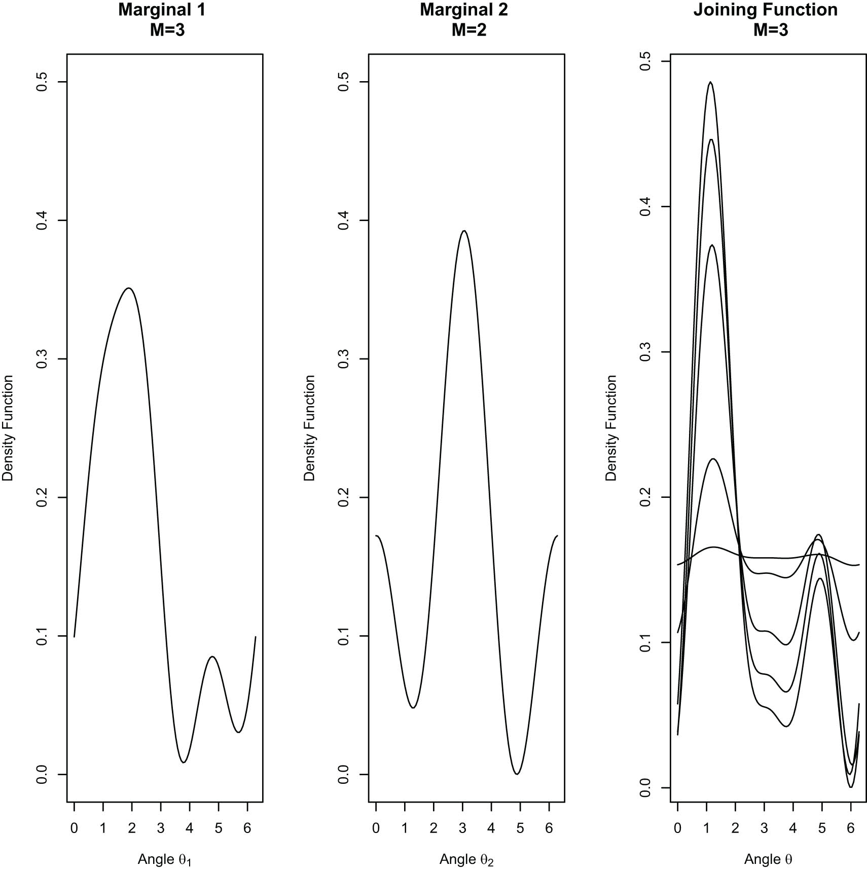
Circular-circular copula model: The first two plots show the marginal NNTS circular densities (
4.2 Circular-circular models
For Johnson and Wehrly’s circular-circular model, we used the same angular joining density and one of the marginal circular densities as that used in the circular-linear model. Figure 1 depicts the plots of the marginal circular densities that correspond to NNTS densities with
NNTS angular joining density circular-circular power study
| Marginals | SS |
|
|
|
|
|
|||||||||
|---|---|---|---|---|---|---|---|---|---|---|---|---|---|---|---|
| RT | PT | WT | ECT | RT | PT | WT | ECT | RT | PT | WT | ECT | ||||
|
|
20 | 0.7 | 0.63 | 87 | 80 | 16 | 38 | 78 | 73 | 11 | 29 | 59 | 61 | 1 | 11 |
|
|
20 | 0.8 | 0.6 | 84 | 81 | 13 | 41 | 72 | 74 | 9 | 28 | 57 | 57 | 3 | 10 |
| 20 | 0.9 | 0.59 | 81 | 79 | 20 | 36 | 76 | 67 | 15 | 28 | 46 | 49 | 5 | 7 | |
| 20 | 0.99 | 0.25 | 34 | 33 | 19 | 15 | 26 | 23 | 13 | 12 | 10 | 8 | 7 | 4 | |
| 20 | 0.9999 | 0.13 | 11 | 13 | 12 | 10 | 7 | 7 | 7 | 10 | 1 | 0 | 1 | 1 | |
| 50 | 0.7 | 0.45 | 100 | 100 | 16 | 88 | 99 | 99 | 7 | 63 | 99 | 98 | 1 | 41 | |
| 50 | 0.8 | 0.5 | 100 | 100 | 15 | 91 | 100 | 100 | 5 | 70 | 98 | 98 | 0 | 38 | |
| 50 | 0.9 | 0.49 | 100 | 100 | 28 | 92 | 100 | 100 | 14 | 70 | 100 | 100 | 6 | 34 | |
| 50 | 0.99 | 0.14 | 70 | 73 | 25 | 36 | 55 | 63 | 16 | 17 | 36 | 36 | 7 | 6 | |
| 50 | 0.9999 | 0.05 | 17 | 14 | 9 | 12 | 6 | 6 | 4 | 3 | 0 | 1 | 3 | 1 | |
| 100 | 0.7 | 0.42 | 100 | 100 | 13 | 100 | 100 | 100 | 9 | 100 | 100 | 100 | 3 | 92 | |
| 100 | 0.8 | 0.47 | 100 | 100 | 17 | 100 | 100 | 100 | 9 | 100 | 100 | 100 | 2 | 93 | |
| 100 | 0.9 | 0.46 | 100 | 100 | 38 | 100 | 100 | 100 | 28 | 100 | 100 | 100 | 10 | 96 | |
| 100 | 0.99 | 0.12 | 90 | 95 | 32 | 60 | 83 | 92 | 23 | 41 | 64 | 85 | 10 | 15 | |
| 100 | 0.9999 | 0.02 | 9 | 14 | 17 | 8 | 4 | 7 | 7 | 1 | 3 | 1 | 1 | 0 | |
| 200 | 0.7 | 0.43 | 100 | 100 | 25 | 100 | 100 | 100 | 19 | 100 | 100 | 100 | 6 | 100 | |
| 200 | 0.8 | 0.48 | 100 | 100 | 18 | 100 | 100 | 100 | 12 | 100 | 100 | 100 | 6 | 100 | |
| 200 | 0.9 | 0.45 | 100 | 100 | 51 | 100 | 100 | 100 | 45 | 100 | 100 | 100 | 21 | 100 | |
| 200 | 0.99 | 0.1 | 100 | 100 | 42 | 86 | 100 | 100 | 31 | 80 | 99 | 99 | 15 | 40 | |
| 200 | 0.9999 | 0.01 | 8 | 10 | 12 | 9 | 4 | 6 | 6 | 4 | 0 | 0 | 2 | 1 | |
The powers of the proposed test implemented using the ART and APT circular uniformity tests, the WT, and the empirical copula test (ECT) are compared when simulating 100 times samples of sizes 20, 50, 100, and 200 from a Johnson and Wehrly circular-circular density function constructed from an NNTS angular joining density with
4.3 Linear-linear models
Tables 3 and 4 list the powers of different tests while simulating samples from a bivariate distribution in which both variables are linear. In the first case, a Gaussian copula was used, and in the second case, a Frank copula was used.
Gaussian copula linear-linear power study
| Marginals | SS |
|
|
|
|
|
|||||||||
|---|---|---|---|---|---|---|---|---|---|---|---|---|---|---|---|
| ART | APT | WT | ECT | ART | APT | WT | ECT | ART | APT | WT | ECT | ||||
|
|
20 | 0.99 | 1 | 100 | 100 | 100 | 100 | 100 | 100 | 100 | 100 | 100 | 100 | 100 | 100 |
|
|
20 | 0.75 | 0.57 | 75 | 69 | 98 | 97 | 68 | 60 | 92 | 92 | 50 | 45 | 83 | 75 |
| 20 | 0.5 | 0.25 | 38 | 36 | 64 | 60 | 24 | 25 | 51 | 47 | 9 | 7 | 40 | 24 | |
| 20 | 0.25 | 0.15 | 17 | 20 | 33 | 29 | 10 | 8 | 24 | 15 | 3 | 4 | 9 | 3 | |
| 20 | 0 | 0.14 | 10 | 14 | 12 | 10 | 7 | 9 | 8 | 5 | 0 | 0 | 2 | 3 | |
| 50 | 0.99 | 1 | 100 | 100 | 100 | 100 | 100 | 100 | 100 | 100 | 100 | 100 | 100 | 100 | |
| 50 | 0.75 | 0.48 | 99 | 98 | 100 | 100 | 99 | 96 | 100 | 100 | 91 | 89 | 100 | 100 | |
| 50 | 0.5 | 0.14 | 57 | 51 | 93 | 94 | 46 | 38 | 87 | 90 | 23 | 21 | 71 | 85 | |
| 50 | 0.25 | 0.06 | 18 | 17 | 52 | 42 | 10 | 7 | 42 | 28 | 2 | 1 | 14 | 15 | |
| 50 | 0 | 0.05 | 7 | 6 | 11 | 8 | 1 | 3 | 6 | 4 | 1 | 0 | 4 | 0 | |
| 100 | 0.99 | 1 | 100 | 100 | 100 | 100 | 100 | 100 | 100 | 100 | 100 | 100 | 100 | 100 | |
| 100 | 0.75 | 0.43 | 100 | 100 | 100 | 100 | 100 | 100 | 100 | 100 | 99 | 99 | 100 | 100 | |
| 100 | 0.5 | 0.11 | 79 | 76 | 97 | 99 | 72 | 61 | 96 | 99 | 50 | 43 | 94 | 98 | |
| 100 | 0.25 | 0.03 | 32 | 30 | 71 | 69 | 20 | 15 | 58 | 55 | 4 | 5 | 37 | 36 | |
| 100 | 0 | 0.02 | 8 | 12 | 13 | 10 | 4 | 3 | 10 | 5 | 1 | 1 | 4 | 1 | |
| 200 | 0.99 | 1 | 100 | 100 | 100 | 100 | 100 | 100 | 100 | 100 | 100 | 100 | 100 | 100 | |
| 200 | 0.75 | 0.4 | 100 | 100 | 100 | 100 | 100 | 100 | 100 | 100 | 100 | 100 | 100 | 100 | |
| 200 | 0.5 | 0.08 | 99 | 98 | 100 | 100 | 97 | 97 | 100 | 100 | 88 | 82 | 100 | 100 | |
| 200 | 0.25 | 0.02 | 33 | 27 | 90 | 94 | 21 | 24 | 86 | 90 | 10 | 7 | 63 | 74 | |
| 200 | 0 | 0.01 | 10 | 13 | 13 | 6 | 6 | 7 | 7 | 1 | 1 | 1 | 1 | 0 | |
|
|
20 | 0.99 | 1 | 100 | 100 | 100 | 100 | 100 | 100 | 100 | 100 | 100 | 100 | 100 | 100 |
|
|
20 | 0.75 | 0.6 | 81 | 75 | 99 | 97 | 70 | 64 | 99 | 93 | 50 | 37 | 94 | 72 |
| 20 | 0.5 | 0.26 | 27 | 21 | 73 | 66 | 19 | 13 | 65 | 54 | 7 | 4 | 42 | 25 | |
| 20 | 0.25 | 0.14 | 13 | 10 | 38 | 21 | 4 | 7 | 25 | 12 | 1 | 2 | 11 | 2 | |
| 20 | 0 | 0.15 | 13 | 8 | 15 | 7 | 4 | 6 | 8 | 5 | 1 | 1 | 2 | 2 | |
| 50 | 0.99 | 1 | 100 | 100 | 100 | 100 | 100 | 100 | 100 | 100 | 100 | 100 | 100 | 100 | |
| 50 | 0.75 | 0.49 | 99 | 99 | 100 | 100 | 98 | 97 | 100 | 100 | 96 | 92 | 100 | 100 | |
| 50 | 0.5 | 0.12 | 59 | 51 | 99 | 95 | 40 | 40 | 98 | 92 | 26 | 22 | 92 | 75 | |
| 50 | 0.25 | 0.05 | 19 | 15 | 58 | 45 | 8 | 11 | 47 | 32 | 1 | 1 | 28 | 13 | |
| 50 | 0 | 0.04 | 5 | 8 | 13 | 10 | 1 | 5 | 6 | 5 | 1 | 1 | 1 | 3 | |
| 100 | 0.99 | 1 | 100 | 100 | 100 | 100 | 100 | 100 | 100 | 100 | 100 | 100 | 100 | 100 | |
| 100 | 0.75 | 0.44 | 100 | 100 | 100 | 100 | 100 | 100 | 100 | 100 | 100 | 100 | 100 | 100 | |
| 100 | 0.5 | 0.1 | 81 | 75 | 100 | 100 | 69 | 66 | 100 | 100 | 47 | 44 | 99 | 100 | |
| 100 | 0.25 | 0.03 | 23 | 18 | 80 | 71 | 12 | 11 | 75 | 56 | 3 | 4 | 57 | 33 | |
| 100 | 0 | 0.02 | 4 | 6 | 9 | 5 | 1 | 5 | 4 | 1 | 0 | 0 | 2 | 0 | |
| 200 | 0.99 | 1 | 100 | 100 | 100 | 100 | 100 | 100 | 100 | 100 | 100 | 100 | 100 | 100 | |
| 200 | 0.75 | 0.4 | 100 | 100 | 100 | 100 | 100 | 100 | 100 | 100 | 100 | 100 | 100 | 100 | |
| 200 | 0.5 | 0.09 | 98 | 97 | 100 | 100 | 96 | 92 | 100 | 100 | 88 | 83 | 100 | 100 | |
| 200 | 0.25 | 0.02 | 41 | 28 | 98 | 93 | 22 | 19 | 93 | 90 | 9 | 8 | 83 | 79 | |
| 200 | 0 | 0.01 | 11 | 11 | 10 | 11 | 8 | 5 | 5 | 5 | 0 | 0 | 0 | 2 | |
|
|
20 | 0.99 | 1 | 100 | 100 | 100 | 100 | 100 | 100 | 100 | 100 | 100 | 100 | 100 | 100 |
|
|
20 | 0.75 | 0.57 | 75 | 69 | 85 | 97 | 68 | 60 | 77 | 92 | 50 | 45 | 60 | 80 |
| 20 | 0.5 | 0.25 | 38 | 36 | 42 | 60 | 24 | 25 | 35 | 47 | 9 | 7 | 23 | 26 | |
| 20 | 0.25 | 0.15 | 17 | 20 | 18 | 30 | 10 | 8 | 15 | 14 | 3 | 4 | 12 | 6 | |
| 20 | 0 | 0.14 | 10 | 14 | 16 | 10 | 7 | 9 | 13 | 5 | 0 | 0 | 7 | 4 | |
| 50 | 0.99 | 1 | 100 | 100 | 100 | 100 | 100 | 100 | 100 | 100 | 100 | 100 | 100 | 100 | |
| 50 | 0.75 | 0.48 | 99 | 98 | 93 | 100 | 99 | 96 | 90 | 100 | 91 | 89 | 81 | 100 | |
| 50 | 0.5 | 0.14 | 57 | 51 | 55 | 94 | 46 | 38 | 43 | 90 | 23 | 21 | 31 | 85 | |
| 50 | 0.25 | 0.06 | 18 | 17 | 18 | 42 | 10 | 7 | 15 | 28 | 2 | 1 | 9 | 15 | |
| 50 | 0 | 0.05 | 7 | 6 | 8 | 8 | 1 | 3 | 7 | 4 | 1 | 0 | 5 | 0 | |
| 100 | 0.99 | 1 | 100 | 100 | 100 | 100 | 100 | 100 | 100 | 100 | 100 | 100 | 100 | 100 | |
| 100 | 0.75 | 0.43 | 100 | 100 | 96 | 100 | 100 | 100 | 95 | 100 | 99 | 99 | 88 | 100 | |
| 100 | 0.5 | 0.11 | 79 | 76 | 63 | 99 | 72 | 61 | 53 | 99 | 50 | 43 | 40 | 98 | |
| 100 | 0.25 | 0.03 | 32 | 30 | 21 | 69 | 20 | 15 | 16 | 55 | 4 | 5 | 11 | 36 | |
| 100 | 0 | 0.02 | 8 | 12 | 10 | 10 | 4 | 3 | 6 | 5 | 1 | 1 | 2 | 1 | |
| 200 | 0.99 | 1 | 100 | 100 | 100 | 100 | 100 | 100 | 100 | 100 | 100 | 100 | 100 | 100 | |
| 200 | 0.75 | 0.4 | 100 | 100 | 96 | 100 | 100 | 100 | 95 | 100 | 100 | 100 | 89 | 100 | |
| 200 | 0.5 | 0.08 | 99 | 98 | 67 | 100 | 97 | 97 | 62 | 100 | 88 | 82 | 44 | 100 | |
| 200 | 0.25 | 0.02 | 33 | 27 | 19 | 94 | 21 | 24 | 13 | 90 | 10 | 7 | 10 | 74 | |
| 200 | 0 | 0.01 | 10 | 13 | 5 | 6 | 6 | 7 | 5 | 1 | 1 | 1 | 2 | 0 | |
The powers of the proposed test implemented using the ART and APT circular uniformity tests, the WT and the ECT tests are compared when simulating 100 times samples of sizes 20, 50, 100, and 200 from a linear-linear density function constructed from a Gaussian copula and three different marginals (exponential, Gaussian, and Cauchy). The Gaussian copula is defined with an equicorrelated correlation matrix with five different common correlation values of 0, 0.25, 0.5, 0.75, and 0.99. The case with common correlation equal to zero corresponds to the null independence model.
Frank copula linear-linear power study
| Marginals | SS |
|
|
|
|
|
|||||||||
|---|---|---|---|---|---|---|---|---|---|---|---|---|---|---|---|
| ART | APT | WT | ECT | ART | APT | WT | ECT | ART | APT | WT | ECT | ||||
|
|
20 | 50 | 1 | 100 | 100 | 100 | 100 | 100 | 100 | 100 | 100 | 100 | 100 | 100 | 100 |
|
|
20 | 15 | 0.95 | 100 | 100 | 100 | 100 | 100 | 99 | 100 | 100 | 99 | 97 | 98 | 100 |
| 20 | 10 | 0.83 | 97 | 95 | 98 | 100 | 96 | 90 | 97 | 99 | 88 | 78 | 92 | 98 | |
| 20 | 5 | 0.4 | 55 | 48 | 72 | 89 | 46 | 41 | 62 | 77 | 31 | 19 | 38 | 59 | |
| 20 | 0 | 0.14 | 14 | 10 | 4 | 6 | 4 | 2 | 1 | 3 | 1 | 0 | 0 | 0 | |
| 50 | 50 | 1 | 100 | 100 | 100 | 100 | 100 | 100 | 100 | 100 | 100 | 100 | 100 | 100 | |
| 50 | 15 | 0.99 | 100 | 100 | 100 | 100 | 100 | 100 | 100 | 100 | 100 | 100 | 100 | 100 | |
| 50 | 10 | 0.9 | 100 | 100 | 100 | 100 | 100 | 100 | 100 | 100 | 100 | 100 | 100 | 100 | |
| 50 | 5 | 0.34 | 97 | 89 | 95 | 100 | 94 | 84 | 94 | 99 | 81 | 67 | 83 | 99 | |
| 50 | 0 | 0.05 | 14 | 12 | 3 | 13 | 6 | 7 | 2 | 7 | 1 | 2 | 0 | 1 | |
| 100 | 50 | 1 | 100 | 100 | 100 | 100 | 100 | 100 | 100 | 100 | 100 | 100 | 100 | 100 | |
| 100 | 15 | 1 | 100 | 100 | 100 | 100 | 100 | 100 | 100 | 100 | 100 | 100 | 100 | 100 | |
| 100 | 10 | 0.89 | 100 | 100 | 100 | 100 | 100 | 100 | 100 | 100 | 100 | 100 | 100 | 100 | |
| 100 | 5 | 0.31 | 100 | 100 | 100 | 100 | 100 | 100 | 100 | 100 | 100 | 97 | 100 | 100 | |
| 100 | 0 | 0.02 | 9 | 9 | 3 | 9 | 4 | 4 | 2 | 4 | 1 | 0 | 2 | 0 | |
| 200 | 50 | 1 | 100 | 100 | 100 | 100 | 100 | 100 | 100 | 100 | 100 | 100 | 100 | 100 | |
| 200 | 15 | 1 | 100 | 100 | 100 | 100 | 100 | 100 | 100 | 100 | 100 | 100 | 100 | 100 | |
| 200 | 10 | 0.88 | 100 | 100 | 100 | 100 | 100 | 100 | 100 | 100 | 100 | 100 | 100 | 100 | |
| 200 | 5 | 0.29 | 100 | 100 | 100 | 100 | 100 | 100 | 100 | 100 | 100 | 100 | 100 | 100 | |
| 200 | 0 | 0.01 | 8 | 10 | 5 | 8 | 4 | 5 | 2 | 6 | 1 | 1 | 0 | 2 | |
|
|
20 | 50 | 1 | 100 | 100 | 100 | 100 | 100 | 100 | 100 | 100 | 100 | 100 | 100 | 100 |
|
|
20 | 15 | 0.95 | 100 | 100 | 100 | 100 | 100 | 99 | 100 | 100 | 99 | 97 | 100 | 100 |
| 20 | 10 | 0.83 | 97 | 95 | 100 | 100 | 96 | 90 | 99 | 99 | 88 | 78 | 99 | 97 | |
| 20 | 5 | 0.4 | 55 | 48 | 94 | 90 | 46 | 41 | 88 | 72 | 31 | 19 | 69 | 54 | |
| 20 | 0 | 0.14 | 14 | 10 | 10 | 6 | 4 | 2 | 5 | 3 | 1 | 0 | 1 | 0 | |
| 50 | 50 | 1 | 100 | 100 | 100 | 100 | 100 | 100 | 100 | 100 | 100 | 100 | 100 | 100 | |
| 50 | 15 | 0.99 | 100 | 100 | 100 | 100 | 100 | 100 | 100 | 100 | 100 | 100 | 100 | 100 | |
| 50 | 10 | 0.9 | 100 | 100 | 100 | 100 | 100 | 100 | 100 | 100 | 100 | 100 | 100 | 100 | |
| 50 | 5 | 0.34 | 97 | 89 | 99 | 100 | 94 | 84 | 99 | 99 | 81 | 67 | 99 | 99 | |
| 50 | 0 | 0.05 | 14 | 12 | 13 | 13 | 6 | 7 | 6 | 7 | 1 | 2 | 0 | 1 | |
| 100 | 50 | 1 | 100 | 100 | 100 | 100 | 100 | 100 | 100 | 100 | 100 | 100 | 100 | 100 | |
| 100 | 15 | 1 | 100 | 100 | 100 | 100 | 100 | 100 | 100 | 100 | 100 | 100 | 100 | 100 | |
| 100 | 10 | 0.89 | 100 | 100 | 100 | 100 | 100 | 100 | 100 | 100 | 100 | 100 | 100 | 100 | |
| 100 | 5 | 0.31 | 100 | 100 | 100 | 100 | 100 | 100 | 100 | 100 | 100 | 97 | 100 | 100 | |
| 100 | 0 | 0.02 | 9 | 9 | 5 | 9 | 4 | 4 | 3 | 4 | 1 | 0 | 0 | 0 | |
| 200 | 50 | 1 | 100 | 100 | 100 | 100 | 100 | 100 | 100 | 100 | 100 | 100 | 100 | 100 | |
| 200 | 15 | 1 | 100 | 100 | 100 | 100 | 100 | 100 | 100 | 100 | 100 | 100 | 100 | 100 | |
| 200 | 10 | 0.88 | 100 | 100 | 100 | 100 | 100 | 100 | 100 | 100 | 100 | 100 | 100 | 100 | |
| 200 | 5 | 0.29 | 100 | 100 | 100 | 100 | 100 | 100 | 100 | 100 | 100 | 100 | 100 | 100 | |
| 200 | 0 | 0.01 | 8 | 10 | 9 | 8 | 4 | 5 | 6 | 6 | 1 | 1 | 1 | 2 | |
|
|
20 | 50 | 1 | 100 | 100 | 95 | 100 | 100 | 100 | 92 | 100 | 100 | 100 | 91 | 100 |
|
|
20 | 15 | 0.95 | 100 | 100 | 81 | 100 | 100 | 99 | 73 | 100 | 99 | 97 | 62 | 100 |
| 20 | 10 | 0.83 | 97 | 95 | 71 | 100 | 96 | 90 | 64 | 99 | 88 | 78 | 47 | 97 | |
| 20 | 5 | 0.4 | 55 | 48 | 42 | 90 | 46 | 41 | 33 | 72 | 31 | 19 | 19 | 54 | |
| 20 | 0 | 0.14 | 14 | 10 | 12 | 6 | 4 | 2 | 7 | 3 | 1 | 0 | 2 | 0 | |
| 50 | 50 | 1 | 100 | 100 | 98 | 100 | 100 | 100 | 95 | 100 | 100 | 100 | 93 | 100 | |
| 50 | 15 | 0.99 | 100 | 100 | 81 | 100 | 100 | 100 | 72 | 100 | 100 | 100 | 62 | 100 | |
| 50 | 10 | 0.9 | 100 | 100 | 66 | 100 | 100 | 100 | 63 | 100 | 100 | 100 | 52 | 100 | |
| 50 | 5 | 0.34 | 97 | 89 | 43 | 100 | 94 | 84 | 38 | 99 | 81 | 67 | 25 | 99 | |
| 50 | 0 | 0.05 | 14 | 12 | 12 | 13 | 6 | 7 | 9 | 7 | 1 | 2 | 4 | 1 | |
| 100 | 50 | 1 | 100 | 100 | 92 | 100 | 100 | 100 | 89 | 100 | 100 | 100 | 81 | 100 | |
| 100 | 15 | 1 | 100 | 100 | 70 | 100 | 100 | 100 | 65 | 100 | 100 | 100 | 49 | 100 | |
| 100 | 10 | 0.89 | 100 | 100 | 64 | 100 | 100 | 100 | 54 | 100 | 100 | 100 | 35 | 100 | |
| 100 | 5 | 0.31 | 100 | 100 | 32 | 100 | 100 | 100 | 25 | 100 | 100 | 97 | 20 | 100 | |
| 100 | 0 | 0.02 | 9 | 9 | 7 | 9 | 4 | 4 | 5 | 4 | 1 | 0 | 5 | 0 | |
| 200 | 50 | 1 | 100 | 100 | 86 | 100 | 100 | 100 | 82 | 100 | 100 | 100 | 77 | 100 | |
| 200 | 15 | 1 | 100 | 100 | 62 | 100 | 100 | 100 | 55 | 100 | 100 | 100 | 43 | 100 | |
| 200 | 10 | 0.88 | 100 | 100 | 49 | 100 | 100 | 100 | 42 | 100 | 100 | 100 | 35 | 100 | |
| 200 | 5 | 0.29 | 100 | 100 | 30 | 100 | 100 | 100 | 26 | 100 | 100 | 100 | 14 | 100 | |
| 200 | 0 | 0.01 | 8 | 10 | 5 | 9 | 4 | 5 | 4 | 7 | 1 | 1 | 2 | 2 | |
The powers of the proposed test implemented using the ART and APT circular uniformity tests, the WT and the ECT are compared when simulating 100 times samples of sizes 20, 50, 100, and 200 from a linear-linear density function constructed from a Frank copula and three different marginals (exponential, Gaussian, and Cauchy). The Frank copula is defined with five different values of the dependence parameter
4.3.1 Bivariate Gaussian copula
The bivariate Gaussian (normal) copula correspond to a multivariate distribution, which is defined as follows:
where
Table 3 compares the powers of the proposed independence test when using a ART and APT circular uniformity tests with respect to those of the WT and ECT independence tests when using simulated samples from a bivariate linear-linear distribution with a Gaussian copula and three different cases of marginal distributions following Herwatz and Maxand [23]: exponential, Gaussian, and Cauchy. For the Gaussian copula, we considered five different values of the correlation coefficient
4.3.2 Bivariate Frank copula
The Frank bivariate copula is defined as follows:
where
5 Application to real circular-circular and circular-linear data
5.1 Test of bivariate independence
5.1.1 Circular-linear real examples
Figure 2 depicts the scatterplots of the considered real examples. We applied the proposed independence test to the circular-linear data on wind direction (circular variable) and ozone concentration (linear variable) originally analyzed by Johnson and Wehrly [28], and later included them as dataset B.18 in Fisher [17]. A total of 19 measurements were taken at a weather station in Milwaukee at 6 o’clock in the morning every fourth day starting on April 18 and ending on June 29, 1975. The scatterplot of this data is included in the top left plot of Figure 2, which presents the values of the wind direction and ozone concentration, further indicating a possible positive association between the circular and linear variables and considering the periodicity of the circular random variable. By applying the Pycke and Rayleigh circular uniformity tests to the difference modulus 2
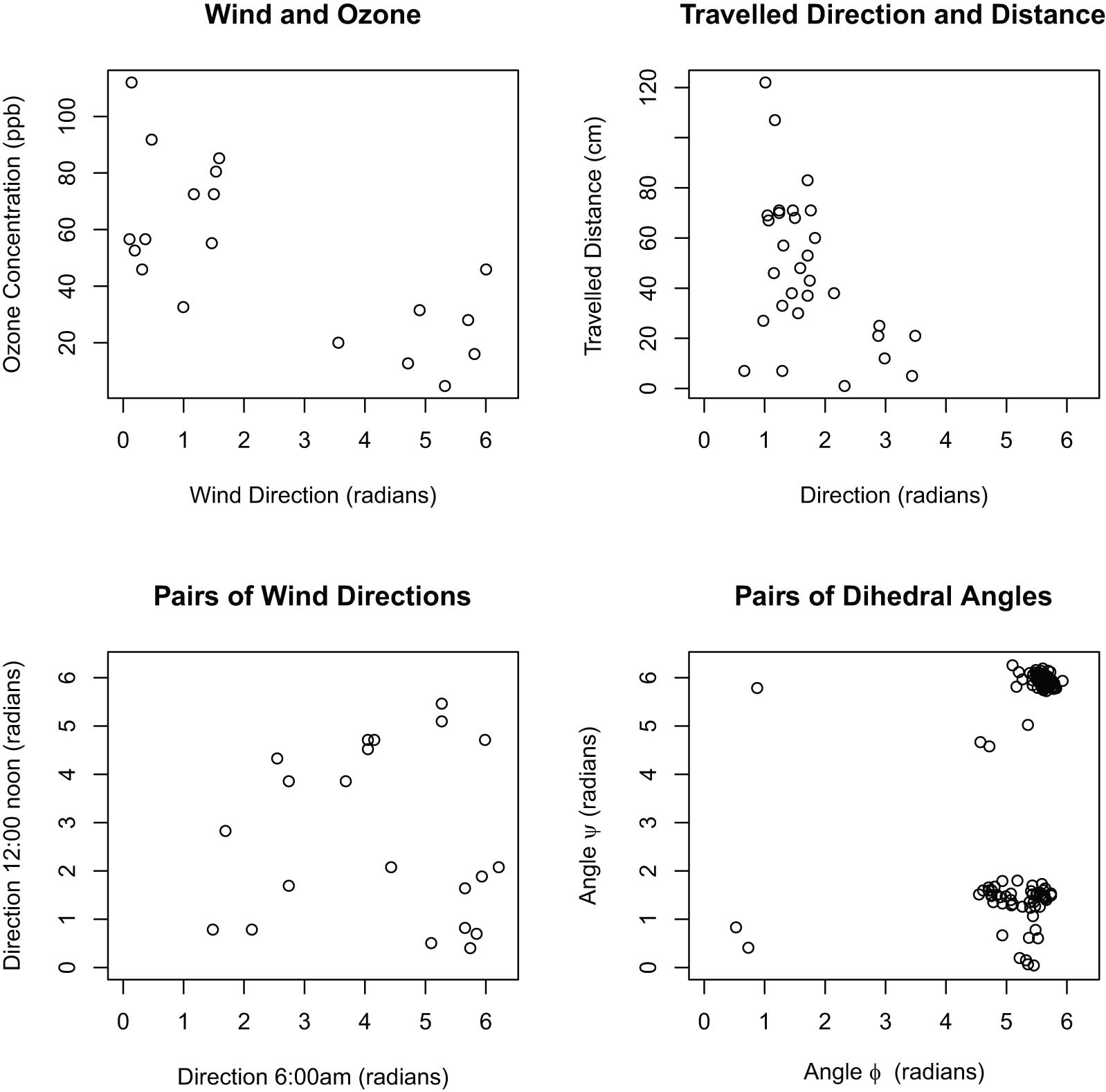
Scatterplots of the circular-linear (upper plots) and circular-circular (lower plots) real datasets. The upper left scatterplot shows the wind direction (relative to north) and ozone concentration (ppb) datapoints of the dataset of Johnson and Wehrly (1977). The upper right plot corresponds to the small blue periwinkles dataset on travelled distance (cm) and direction analyzed by Fisher (1993). The bottom left plot corresponds to the Johnson and Wehrly (1977) dataset on pairs of wind directions (relative to north) at 6:00 am and 12:00 noon in a weather monitoring station. At last, the bottom right includes the pairs of dihedral angles in segments alanine-alanine-alanine of proteins originally analyzed by Fernández-Durán (2007).
A second example analyzed by Fisher [17] is a dataset on the directions and distances travelled by 31 small blue periwinkles after undergoing transplantation from their normal place of living. The top-right plot depicted in Figure 2 includes the scatterplot for this dataset, further indicating a possible negative association between the direction and travelled distance. When applying the uniformity test to the sum modulus 2
5.1.2 Circular-circular real examples
The first example in the circular-circular test of independence corresponds to pairs of wind directions measured at a weather monitoring station at Milwaukee. The measurements were taken at 6:00 and 12:00 o’clock for 21 consecutive days and were originally included in Johnson and Wehrly [28]. The bottom-left plot depicted in Figure 2 includes a scatterplot of the pairs of wind directions, which indicates a possible positive association between the two angles. Fisher [17] listed this dataset as the B.21 dataset, and the main conclusion of Fisher [17] was that there exists a strong positive association between the wind directions when applying a hypothesis test based on a circular-circular correlation coefficient. When applying the proposed methodology to the difference modulus 2
The second example corresponds to 233 pairs (
6 Conclusion
By using the result that the sum modulus 2
Acknowledgments
We express our sincere gratitude to the Asociación Mexicana de Cultura, A.C. for their support.
-
Funding information: No funding was received to assist with the preparation of this manuscript.
-
Conflict of interest: The authors have no conflict of interest to declare that are relevant to the content of this article.
References
[1] Agostinelli, C., & Lund, U. (2017). R package ‘circular’: Circular Statistics (version 0.4-93). https://r-forge.r-project.org/projects/circular/. Search in Google Scholar
[2] Berrett, T. B., & Samworth, R. J. (2019). Nonparametric independence testing via mutual information. Biometrika, 106(3), 547–556. 10.1093/biomet/asz024Search in Google Scholar
[3] Blum, J. R., Keifer, J., & Rosenblatt, M. (1961). Distribution Free Tests of Independence Based on the Sample Distribution Function. Annals of Mathematical Statistics, 32(2), 485–498. 10.1214/aoms/1177705055Search in Google Scholar
[4] Cinar, O., & Viechtbauer, W. (2022). The poolr Package for Combining Independent and Dependent p values. Journal of Statistical Software, 101, 1–42. 10.18637/jss.v101.i01Search in Google Scholar
[5] Csörgö, S. (1985). Testing for independence by the empirical characteristic function. Journal of Multivariate Analysis, 16, 290–299. 10.1016/0047-259X(85)90022-3Search in Google Scholar
[6] Deheuvels, P. (1981). An asymptotic decomposition for multivariate distribution-free tests of independence. Journal of Multivariate Analysis, 11(1), 102–113. 10.1016/0047-259X(81)90136-6Search in Google Scholar
[7] DeWet, T.( 1980). Cramér-von Mises Tests for Independence. Journal of Multivariate Analysis, 10, 38–50. 10.1016/0047-259X(80)90080-9Search in Google Scholar
[8] Einmahl, J. H., & McKeague, I. W. (2003). Empirical likelihood based hypothesis testing. Bernoulli, 9(2), 267–290. 10.3150/bj/1068128978Search in Google Scholar
[9] Fernández-Durán, J. J. (2004a). Modelling ground-level ozone concentration using copulas. In G. J., Erickson, & Y., Zhai (Eds.) 23rd International Workshop on Bayesian Inference and Maximum Entropy Methods in Science and Engineering, Proceedings of the Conference held 3-8 August, 2003 in Jackson Hole, Wyoming. AIP Conference Proceeding (Vol. 707, pp. 406–413). New York: American Institute of Physics. 10.1063/1.1751383Search in Google Scholar
[10] Fernández-Durán, J. J. (2004b). Circular distributions based on nonnegative trigonometric sums. Biometrics, 60, 499–503. 10.1111/j.0006-341X.2004.00195.xSearch in Google Scholar PubMed
[11] Fernández-Durán, J. J. (2007). Models for circular-linear and circular-circular data constructed from circular distributions based on nonnegative trigonometric sums. Biometrics, 63(2), 579–585. 10.1111/j.1541-0420.2006.00716.xSearch in Google Scholar PubMed
[12] Fernández-Durán, J. J., & Gregorio-Domínguez, M. M. (2010). Maximum likelihood estimation of nonnegative trigonometric sums models using a Newton-like algorithm on manifolds. Electronic Journal of Statistics, 4, 1402–10. 10.1214/10-EJS587Search in Google Scholar
[13] Fernández-Durán, J. J., & Gregorio-Domínguez, M. M. (2016). CircNNTSR: An R package for the statistical analysis of circular, multivariatecircular, and spherical data using nonnegative trigonometric sums. Journal of Statistical Software, 70, 1–19. 10.18637/jss.v070.i06Search in Google Scholar
[14] Fisher, N. I., & Lee, A. J. (1981). Nonparametric measures of angular-linear association. Biometrika, 68, 629–636. 10.1093/biomet/68.3.629Search in Google Scholar
[15] Fisher, N. I., & Lee, A. J. (1982). Nonparametric measures of angular-angular association. Biometrika, 69, 315–321. 10.1093/biomet/69.2.315Search in Google Scholar
[16] Fisher, N. I., & Lee, A. J. (1983). A correlation coefficient for circular data. Biometrika, 70, 327–332. 10.1093/biomet/70.2.327Search in Google Scholar
[17] Fisher, N. I.(1993). Statistical analysis of circular data. Cambridge, New York: Cambridge University Press. 10.1017/CBO9780511564345Search in Google Scholar
[18] Fitak, R. R., & Johnsen, S. (2017). Bringing the analysis of animal orientation data full circle: Model-based approaches with maximum likelihood. Journal of Experimental Biology, 220, 3878–3882. 10.1242/jeb.167056Search in Google Scholar PubMed PubMed Central
[19] Genest, C., & Rémillard, B. (2004). Test of independence and randomness based on the empirical copula process. Test, 13, 335–369. 10.1007/BF02595777Search in Google Scholar
[20] Genest, C., & Verret, F. (2005). Locally most powerful rank tests of independence for copula models. Nonparametric Statistics, 17, 521–539. 10.1080/10485250500038926Search in Google Scholar
[21] Genest, C., Nešlehová, J. G., Rémillard, B., & Murphy, O. A. (2019). Testing for independence in arbitrary distributions. Biometrika, 106, 47–68. 10.1093/biomet/asy059Search in Google Scholar
[22] Goeman, J. J., & Solari, A. (2014). Multiple hypothesis testing in genomics. Statistics in Medicine, 33, 1946–1978. 10.1002/sim.6082Search in Google Scholar PubMed
[23] Herwatz, H., & Maxand, S. (2020). Nonparametric tests for independence: A review and comparative simulation study with an application to malnutrition datain India. Statistical Papers, 61, 2175–2201. 10.1007/s00362-018-1026-9Search in Google Scholar
[24] Hoeffding, W. (1948). A non-parametric test of independence. The Annals of Mathematical Statistics, 19(4), 546–557. 10.1214/aoms/1177730150Search in Google Scholar
[25] Hofert, M., Kojadinovic, I., Maechler, M., & Yan, J. (2022). Copula: Multivariate dependence with copulas. R package version 1.1-1. https://CRAN.R-project.org/package=copula. Search in Google Scholar
[26] Jammalamadaka, S. R., & SenGupta, A. (2001). Topics in Circular Statistics. River Edge, N.J.: World Scientific Publishing, Co. 10.1142/4031Search in Google Scholar
[27] Joe, H. (1990). Multivariate entropy measures of multivariate dependence. Journal of the American Statistical Association, 84, 157–164. 10.1080/01621459.1989.10478751Search in Google Scholar
[28] Johnson, R. A., & Wehrly, T. (1977). Measures and models for angular correlation and angular-linear correlation. Journal of the Royal Statistical Society, Series B, 39(2), 222–229. 10.1111/j.2517-6161.1977.tb01619.xSearch in Google Scholar
[29] Kallenberg, W. C. M., & Ledwina, T. (1999). Data driven rank tests for independence. Journal of the American Statistical Association, 94, 285–301. 10.1080/01621459.1999.10473844Search in Google Scholar
[30] Kendall, M. G. (1938). A new measure of rank correlation. Biometrika, 30(1/2), 81–93. 10.1093/biomet/30.1-2.81Search in Google Scholar
[31] Kendall, M. G., & Stuart, A. (1951). The advanced theory of statistics. Inference and Relationship(Vol. 2). New York: Hafner publishing Company. Search in Google Scholar
[32] Kojadinovic, I., & Yan, J. (2010). Modeling multvariate distributions with continuous margins using the copula R package. Journal of Statistical Software, 34(9), 1–20. 10.18637/jss.v034.i09Search in Google Scholar
[33] Landler, L., Ruxton, G. D., & Malkemper, E. P. (2019). The Hermans-Rasson test as a powerful alternative to the Rayleigh test for circular statistics in biology. BMC Ecology, 19, 30. 10.1186/s12898-019-0246-8Search in Google Scholar PubMed PubMed Central
[34] Mardia, K. V., & Kent, J. T. (1991). Rao score tests for goodness of fit and independence. Biometrika, 78(2), 355–363. 10.1093/biomet/78.2.355Search in Google Scholar
[35] Mardia, K. V., & Jupp, P. E. (2000). Directional statistics. Chichester, New York: John Wiley and Sons. 10.1002/9780470316979Search in Google Scholar
[36] Nelsen, R. (1999). An introduction to copulas. New York: Springer Verlag. 10.1007/978-1-4757-3076-0Search in Google Scholar
[37] Pearson, K. (1920). Notes on the history of correlation. Biometrika, 13(1), 25–45. 10.1093/biomet/13.1.25Search in Google Scholar
[38] Pewsey, A., Neuhäuser, M., & Ruxton, G. D. (2013). Circular statistics in R. Oxford, U.K.: Oxford University Press. Search in Google Scholar
[39] Pewsey, A., & Kato, S. (2016). Parametric bootstrap goodness-of-fit testing for Wehrly-Johnson bivariate circular distributions. Statistics and Computing, 26, 1307–1317. 10.1007/s11222-015-9605-2Search in Google Scholar
[40] Pfister, N., Bühlmann, P., Schölkopf, J. N., & Peters, J. (2018). Kernel-based tests for joint independence. Journal of the Royal Statistical Society, Series B, 80(1), 5–31. 10.1111/rssb.12235Search in Google Scholar
[41] Pycke, J-R. (2010). Some tests for uniformity of circular distributions powerful against multimodal alternatives. The Canadian Journal of Statistics, 38, 80–96. 10.1002/cjs.10048Search in Google Scholar
[42] R Core Team. (2021). R: A language and environment for statistical computing. R Foundation for Statistical Computing, Vienna, Austria. http://www.R-project.org/. Search in Google Scholar
[43] Roy, A. (2020). Some Copula-based tests of independence among several random variables having arbitrary probability distributions. Stat, 9(1), e263.10.1002/sta4.263Search in Google Scholar
[44] Roy, A., Ghosh, A. K., Goswami, A., & Murthy, C. A. (2020). Some new Copula based distribution-free tests of independence among several random variables. Sankhya A, 84, 556–596. 10.1007/s13171-020-00207-2Search in Google Scholar
[45] Sklar, A. (1959). Fonctions de Répartition à n Dimensions et Leurs Marges. Publications de laInstitut de Statistique de laUniversité de Paris, 8, 229–231. Search in Google Scholar
[46] Spearman, C. (1904). The proof and measurement of association between two things. The American Journal of Psychology, 15(1), 72–101. 10.2307/1412159Search in Google Scholar
[47] Upton, G. J. G., & Fingleton, B. (1989). Spatial data analysis by Example Vol. 2 (Categorical and Directional Data). Chichester, New York: John Wileyand Sons. Search in Google Scholar
[48] Wehrly, T., & Johnson, R. A. (1980). Bivariate models for dependence of angular observations and a related Markov process. Biometrika, 67(1), 255–256. 10.1093/biomet/67.1.255Search in Google Scholar
[49] Wilks, S. (1935). On the independence of k sets of normally distributed statistical variables. Econometrica, 3, 309–326. 10.2307/1905324Search in Google Scholar
© 2023 the author(s), published by De Gruyter
This work is licensed under the Creative Commons Attribution 4.0 International License.
Articles in the same Issue
- Research Articles
- Joint lifetime modeling with matrix distributions
- Consistency of mixture models with a prior on the number of components
- Mutual volatility transmission between assets and trading places
- Functions operating on several multivariate distribution functions
- An optimal transport-based characterization of convex order
- Test of bivariate independence based on angular probability integral transform with emphasis on circular-circular and circular-linear data
- A link between Kendall’s τ, the length measure and the surface of bivariate copulas, and a consequence to copulas with self-similar support
- Review Article
- Testing for explosive bubbles: a review
- Interview
- When copulas and smoothing met: An interview with Irène Gijbels
- Special Issue on 10 years of Dependence Modeling
- On copulas with a trapezoid support
- Characterization of pre-idempotent Copulas
- Abel-Gontcharoff polynomials, parking trajectories and ruin probabilities
- A nonparametric test for comparing survival functions based on restricted distance correlation
- Constructing models for spherical and elliptical densities