On copulas with a trapezoid support
-
Piotr Jaworski


Abstract
A family of bivariate copulas given by: for
1 Introduction
In recent years, the interest in the construction of multivariate stochastic models describing the dependence among several variables has grown. In particular, the recent financial crises emphasized the necessity of considering models that can serve to better estimate the occurrence of extremal events (see, e.g., [3,6,23] or [13]).
We introduce a new family of bivariate copulas, which are supported not on the whole unit square
The interest in such copulas has aroused from the study of self-similar stochastic processes and the dependence between such processes and their running minima or maxima processes. See [4] or [1] for the Brownian motion case.
In Section 2, we recall the basic notation, the definition of the bivariate copula, and the formulas for its Kendall
In Section 4, we provide five examples of copulas introduced in the previous section. For each one, we calculate tail parameters and Kendall
The proofs of theorems and calculations are relegated to Section 5, which also contains some auxiliary results. In Section 5.1, we proved that the introduced family of functions is a family of copulas. Sections 5.2 and 5.3 deal with the support and absolute continuity. In Sections 5.4 and 5.5, the Kendall
2 Definitions and basic properties
We recall the definition of a bivariate copula; see [24] and [11] for more details.
Definition 1
The function
is called a copula if the following three properties hold:
where the function
is given as follows:
Note that for
By the celebrated Sklar’s theorem, the joint distribution function
Moreover, if
which are uniformly distributed on
The above is a special case of the more general fact: a bivariate copula
Furthermore, when the marginal distribution functions
Kendall
We observe that since copulas are Lipschitz functions, they are differentiable on the complement of at most a zero measure set (Theorem of Rademacher, [21], Section 7.1), and the integral in the formula (1) is well defined for any copula. Similarly, the tail dependence parameters, lower left (LL), lower right (LR), upper left (UL), and upper right (UR), which describe the dependence of random variables in extreme cases, are defined as limits (providing they exist) as follows:
where
3 Novel construction
We introduce a new family of copulas characterized by a functional parameter
is a strictly increasing continuous cumulative distribution function, which is furthermore symmetric
and convex on the half-line
Theorem 1
Let
given by
is a copula.
The proof is postponed to Section 5.1.
The above-introduced copulas are a close analogy of Archimedean copulas, which are also characterized by functions convex on a half-line, [18,22,24]. We recall that a bivariate copula
where
is continuous and decreasing,
is a right-sided inverse of
Note that an Archimedean generator
is a generator of an Archimedean copula.
The other example of a related family of copulas is left truncation invariant (LTI) copulas [5,8, 9,17]. For any
is a generator of an LTI copula
Similarly as in the Archimedean or LTI case, the construction of
Let
Indeed,
For
As follows from the construction of
as shown in Figure 1. We provide a bit stronger result.
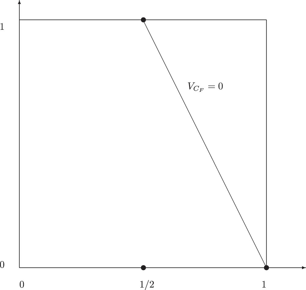
Support of
Theorem 2
Let U and V be representers of a copula
Under some additional slight assumptions, copulas
Theorem 3
Let
If F is not differentiable at 0, then
where g is a nonnegative version of the density of f on the negative half-line, i.e.,
The conditions in the above theorem are also sufficient.
Theorem 4
Let
The proofs of Theorems 2–4 are postponed to Sections 5.2 and 5.3.
4 Examples
To illustrate the concept of “trapezoid” copulas, we provide in this section several examples of the
The upper tail parameters are trivial for all
The lower tail parameters,
exists and equals
For more details, the reader is referred, e.g., to [25]. Note that the regular variation was also studied in the context of the tail behavior of Archimedean copulas [2].
4.1
F
∼
N
(
0
,
1
)
Let
Regular variation index
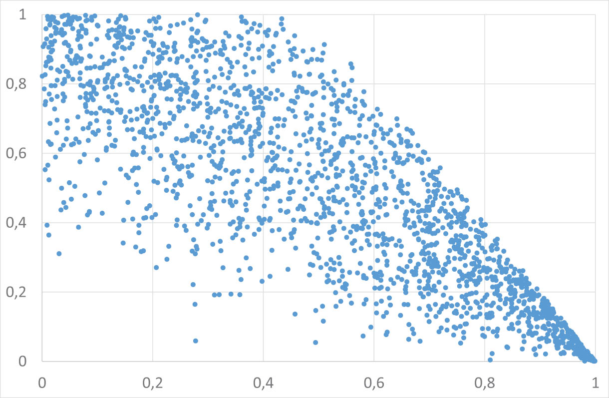
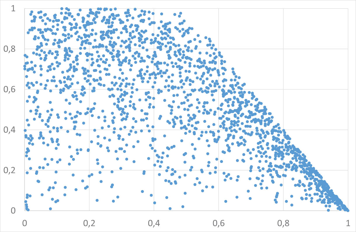
Scatterplot of
Note that
Compare [4] and [1], where the copula of the pair
4.2 Laplace (bi-exponential)
La
(
0
,
1
)
=
Exp
(
1
)
⊕
‒
Exp
(
1
)
Let
Since
we obtain
Regular variation index
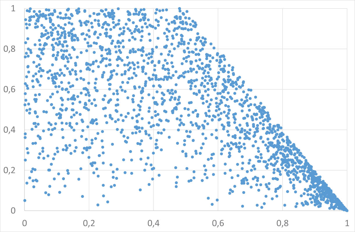
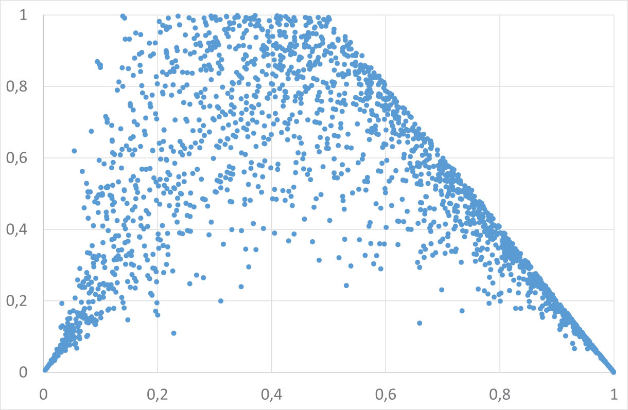
Scatterplot of
4.3 Bi-Pareto,
P
(
I
I
)
(
0
,
1
,
k
)
⊕
‒
P
(
I
I
)
(
0
,
1
,
k
)
Let
Since
we obtain
Regular variation index
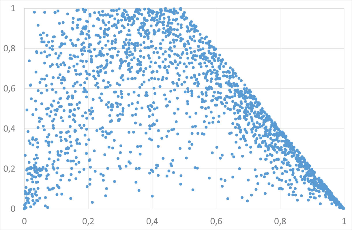
Scatterplot of
4.4
t
-Student,
T
(
n
)
Let
Regular variation index
Scatterplot of
4.5 Extra heavy tail
Let
Since
we obtain
Regular variation index
Scatterplot of
5 Proofs and auxiliary results
5.1 Proof of the Theorem 1
Step 1. Conditions (c1) and (c2) – the easy part.
By direct computation, we obtain
Step 2. Condition (c3).
We follow the approach from [7].
First, we check the continuity of
We introduce an auxiliary function
Since for
We show that
Since
Next, we calculate the right-sided partial derivative of
Let
For
On the other hand, for
We check that for any fixed
is nondecreasing. In more detail:
Since for
and
Furthermore,
Thus, as required, for any
is nondecreasing on the interval
To prove the 2-monotonicity of
For any fixed
We obtain
which implies that
5.2 Support – proof of Theorem 2
We show that the set
contains subsets of the measure close to 1.
Let
Hence,
But taking into account that for any
and substituting
Since
5.3 Density – proofs of Theorems 3 and 4
Proof of Theorem 3
Since
and changing the variables, we obtain that for
Note that for
Similarly, for
Proof of Theorem 4
Let a nonnegative, Borel function
where
is a Borel function. Hence, for a fixed
where
The right side of the equation is an absolutely continuous function of
5.4 Kendall
τ
Theorem 5
Let
where X is a random variable with the cumulative distribution function F and the probability density f.
Proof
Indeed, for
In the following, we show how to calculate Kendall
5.4.1 Kendall
τ
for
N
(
0
,
1
)
generator
We recall that
Hence,
5.4.2 Kendall
τ
for
La
(
0
,
1
)
generator
We recall that for
Hence,
5.4.3 Kendall
τ
for bi-Pareto generator
We recall that for
Hence,
5.4.4 Kendall
τ
for Student generator
We recall that
Hence,
5.4.5 Kendall
τ
for heavy-tailed
F
We recall that for
Hence,
5.5 Spearman
ρ
Theorem 6
Let
where X, Y, and Z are independent and identically distributed (iid) random variables with distribution function F and probability density f.
Proof
We observe that for
5.5.1 Spearman
ρ
for
F
∼
N
(
0
,
1
)
We observe that the joint distribution of independent random variables
We recall that due to Girard’s theorem such volume (taken with respect to the surface measure
where
Therefore,
Finally, we conclude
5.5.2 Spearman
ρ
for Laplace
F
We have
Since
we obtain
5.5.3 Spearman
ρ
by the Monte Carlo method
Thanks to Theorem 6, we may apply Monte Carlo methods to approximate Spearman
For
biPareto
biPareto
biPareto
tStudent
tStudent
tStudent
Extra heavy tail,
5.6 Lower left tail dependence
We say that a copula
where the leading part
and the tail
Note that
provided the limit exists. See [14–16] for more details. The leading part
Proposition 1
Let
Proof
Since
The above convergence is almost uniform in
The regular variation of the function
and the function
Proposition 2
Let
Proof
Since
Since
On the other hand,
We apply the sandwich rule
Proposition 3
Let
Proof
We apply the sandwich rule for small
Since for the copulas with a uniform lower left tail decomposition, the lower left tail parameter exists and equals
we obtain
Corollary 1
Let
5.7 Lower right tail dependence
In order to simplify the calculations, instead of studying the tail behavior of a copula
Let
Indeed,
Hence, the copula
Proposition 4
Let
Proof
We apply the same approach as in the proof of Proposition 1. For
Proposition 5
Let
Proof
Indeed, for
On the other hand,
Proposition 6
Let
and for any
Then, the copula
Proof
We observe that
and
Therefore, for
Since for the copulas, such that their reflections with respect to the line
we obtain the following corollaries.
Corollary 2
Let the survival distribution function
Corollary 3
Let the survival distribution function
Note that for the normal standard distribution function and for Laplace
Furthermore, the existence of
5.8 Left upper tail
The left upper tail of the copula
Since
Since
Inequalities (9) and (10) imply that for sufficiently small positive
Acknowledgments
The author would like to thank the anonymous reviewers for their valuable suggestions and remarks.
-
Funding information: No funding is involved.
-
Conflict of interest: The author state that there is no conflict of interest.
References
[1] Adès, M., Dufour, M., Provost, S., Vachon, M.-C., & Zang, Y. (2022). A class of copulas associated with Brownian motion processes and their maxima. Journal of Applied Mathematics and Computation, 6(1), 96–120. 10.26855/jamc.2022.03.012Search in Google Scholar
[2] Charpentier, A., & Segers, J. (2009). Tails of multivariate Archimedean copulas. Journal of Multivariate Analysis, 100, 1521–1537. 10.1016/j.jmva.2008.12.015Search in Google Scholar
[3] Chavez-Demoulin, V., & Embrechts, P. (2011). An EVT primer for credit risk. In A. Lipton, & A. Rennie, (Eds.), The Oxford handbook of credit derivatives. Oxford UK: Oxford University Press. 10.1093/oxfordhb/9780199546787.013.0014Search in Google Scholar
[4] Da̧browski, K., & Jaworski, P. (2021). On the dependence between a Wiener process and its running maxima and running minima processes. 2021, arXiv:2109.02024 [math.PR]. Search in Google Scholar
[5] DiLascio, F. M. L., Durante, F., & Jaworski, P. (2016). Truncation invariant copulas and a testing procedure. Journal of Statistical Computation and Simulation, 86(12), 2362–2378. 10.1080/00949655.2015.1110820Search in Google Scholar
[6] Donnelly, C., & Embrechts, P. (2010). The devil is in the tails: Actuarial mathematics and the subprime mortgage crisis. Astin Bull., 40(1), 1–33. 10.2143/AST.40.1.2049222Search in Google Scholar
[7] Durante, F., & Jaworski, P. (2010). A new characterization of bivariate copulas. Communications in Statistics - Theory and Methods 39(16), 2901–2912. 10.1080/03610920903151459Search in Google Scholar
[8] Durante, F., & Jaworski, P. (2012). Invariant dependence structure under univariate truncation. Statistics, 46, 263–277. 10.1080/02331888.2010.512977Search in Google Scholar
[9] Durante, F., Jaworski, P., & Mesiar, R. (2011). Invariant dependence structures and Archimedean copulas. Statistics and Probability Letters, 81, 1995–2003. 10.1016/j.spl.2011.08.018Search in Google Scholar
[10] Durante, F., & Sempi, C. (2016). Principles of copula theory. Boca Raton FL: CRS Press. 10.1201/b18674Search in Google Scholar
[11] Embrechts, P. (2009). Copulas: A personal view. Journal of Risk and Insurance, 76, 639–650. 10.1111/j.1539-6975.2009.01310.xSearch in Google Scholar
[12] Embrechts, P., Klü ppelberg, C., & Mikosch, T. (1997). Modeling extremal events for finance and insurance. Berlin: Springer. 10.1007/978-3-642-33483-2Search in Google Scholar
[13] Genest, C., Gendron, M., & Bourdeau-Brien, M. (2009). The advent of copulas in finance. European Journal of Finance, 15, 609–618. 10.1080/13518470802604457Search in Google Scholar
[14] Jaworski, P. (2004). On uniform tail expansions of bivariate copulas. Applicationes Mathematicae, 31, 397–415. 10.4064/am31-4-2Search in Google Scholar
[15] Jaworski, P. (2006). On uniform tail expansions of multivariate copulas and wide convergence of measures. Applicationes Mathematicae, 33, 159–184. 10.4064/am33-2-3Search in Google Scholar
[16] Jaworski, P. (2010). Tail behaviour of copulas. In P. Jaworski, F. Durante, W. Härdle, & T. Rychlik (Eds.), Copula Theory and Its Applications, Proceedings of the Workshop Held in Warsaw, 25–26 September 2009, Lecture Notes in Statistics - Proceedings 198 (pp. 161–186). Berlin: Springer. 10.1007/978-3-642-12465-5_8Search in Google Scholar
[17] Jaworski, P. (2017). On truncation invariant copulas and their estimation. Dependence Modeling, 5, 133–144. 10.1515/demo-2017-0009Search in Google Scholar
[18] Joe, H. (2015). Dependence modeling with copulas. Boca Raton FL: CRS Press. 10.1201/b17116Search in Google Scholar
[19] Joe, H., Li, H., & Nikoloulopoulos, A. (2010). Tail dependence functions and vine copulas. Journal of Multivariate Analysis, 101, 252–270. 10.1016/j.jmva.2009.08.002Search in Google Scholar
[20] Korn, G., & Korn, T. (1968). Mathematical Handbook for Scientists and Engineers. New York: McGraw-Hill. Search in Google Scholar
[21] Łojasiewicz, S. (1988). An introduction to the theory of real functions. A Wiley-Interscience Publication. (3rd edn.). Chichester: John Wiley & Sons Ltd. Search in Google Scholar
[22] McNeil, A. J., & Nešlehová, J. (2009). Multivariate Archimedean copulas, d-monotone functions and l1-norm symmetric distributions. The Annals of Statistics, 37(5b), 3059–3097. 10.1214/07-AOS556Search in Google Scholar
[23] McNeil, A. J., Frey, R., & Embrechts, P. (2005). Quantitative risk management. Concepts, techniques and tools. Princeton Series in Finance. Princeton, NJ: Princeton University Press. Search in Google Scholar
[24] Nelsen, R. B. (2006). An introduction to copulas. Springer series in statistics (2nd edn.). New York: Springer. Search in Google Scholar
[25] Resnick, S. I. (2007). Heavy-Tail phenomena. Probabilistic and statistical modeling. New York: Springer. Search in Google Scholar
© 2023 the author(s), published by De Gruyter
This work is licensed under the Creative Commons Attribution 4.0 International License.
Articles in the same Issue
- Research Articles
- Joint lifetime modeling with matrix distributions
- Consistency of mixture models with a prior on the number of components
- Mutual volatility transmission between assets and trading places
- Functions operating on several multivariate distribution functions
- An optimal transport-based characterization of convex order
- Test of bivariate independence based on angular probability integral transform with emphasis on circular-circular and circular-linear data
- A link between Kendall’s τ, the length measure and the surface of bivariate copulas, and a consequence to copulas with self-similar support
- Review Article
- Testing for explosive bubbles: a review
- Interview
- When copulas and smoothing met: An interview with Irène Gijbels
- Special Issue on 10 years of Dependence Modeling
- On copulas with a trapezoid support
- Characterization of pre-idempotent Copulas
- Abel-Gontcharoff polynomials, parking trajectories and ruin probabilities
- A nonparametric test for comparing survival functions based on restricted distance correlation
- Constructing models for spherical and elliptical densities