A revised model for the effect of nanoparticle mass flux on the thermal instability of a nanofluid layer
-
Ozwah S. Alharbi


Abstract
A revised model of the nanoparticle mass flux is introduced and used to study the thermal instability of the Rayleigh-Benard problem for a horizontal layer of nanofluid heated from below. The motion of nanoparticles is characterized by the effects of thermophoresis and Brownian diffusion. The nanofluid layer is confined between two rigid boundaries. Both boundaries are assumed to be impenetrable to nanoparticles with their distribution being determined from a conservation condition. The material properties of the nanofluid are allowed to depend on the local volume fraction of nanoparticles and are modelled by non-constant constitutive expressions developed by Kanafer and Vafai based on experimental data. The results show that the profile of the nanoparticle volume fraction is of exponential type in the steady-state solution. The resulting equations of the problem constitute an eigenvalue problem which is solved using the Chebyshev tau method. The critical values of the thermal Rayleigh number are calculated for several values of the parameters of the problem. Moreover, the critical eigenvalues obtained were real-valued, which indicates that the mode of instability is via a stationary mode.
1 Introduction
Recently, there has been widespread interest in studying nanofluids and their potential applications. A nanofluid is a mixture of a base fluid such as water or an organic solvent and nanoparticles such as copper, copper oxide, alumina, or multi-walled carbon nanotubes. Many researchers [1,2,3, 4,5] showed that the property of heat transfer in this type of fluid increases substantially compared to ordinary fluids. One of the important investigation of nanofluids is the studying of the thermal instability of this type of fluid. These types of investigations attracted the interests of many researchers. Kim et al. [6] analyzed the thermal instability driven by buoyancy and heat transfer characteristics of nanofluids. Buongiorno [7] proposed a model for convective transport in nanofluids in which the effects of Brownian diffusion and thermophoresis are taken into consideration and showed that only these mechanisms are the most significant drivers of nanoparticle motion. Tzou [8,9] used the model proposed by Buongiorno [7] to study the thermal instability of the Rayleigh-Benard problem for different values of temperatures and nanoparticle volume fractions and showed that for nanofluids, the critical values of the Rayleigh numbers are less by one or two orders of magnitude compared to the corresponding values of base fluids. Kuznetsov and Nield [10] studied analytically the onset of thermal instability in a horizontal layer of a porous medium saturated by a nanofluid using the model proposed by Buongiorno [7]. The same model is used by Nield and Kuznetsov [11] to study the thermal instability of a horizontal layer of nanofluid with a finite depth and concluded that in the case of a typical nanofluid, the main contribution of the nanoparticles is through the effect of buoyancy forces associated with the conservation of the nanoparticles.
The effect of rotation on the thermal instability of nanofluid layer is studied by Yadav et al. [12] analytically. They showed that rotation has a stabilizing effect depending on the values of the parameters of the problem. Yadav et al. [13] studied the effect of a vertical magnetic field on the thermal instability of a horizontal layer of nanofluid and showed that the magnetic field has a stabilizing effect. The joint effect of both rotation and magnetic field on the thermal instability of a nanofluid layer is investigated by Mahajan and Arora [14]. Nield and Kuznetsov [15] revised their paper [11] and changed the boundary conditions of the nanoparticle volume fraction to boundary conditions on the diffusive mass flux of nanoparticles which is physically more realistic. They showed that with the new boundary conditions, oscillatory convection cannot occur and the effect of nanoparticles on non-oscillatory convection is destabilizing. According to this study, most investigations focusing on the thermal instability of a horizontal nanofluid layer employed this revised model to analyze several problems (Agarwal et al. [16], Yadav et al. [17], Agarwal and Rana [18], Abdullah and Lindsay [19], Abdullah et al. [20], Rana et al. [21], Ahuja and Gupta [22]).
It is noted that all the studies [11,12,13, 14,15,16, 17,18,19, 20,21,22] assumed that Brownian and thermophoresis diffusions are constants in the expression of the diffusive mass flux of the nanoparticles and that the material properties of nanofluid such as effective thermal conductivity and effective viscosity behave as parameters across the nanofluid layer. As a result of these assumptions the gradient steady-state distributions of temperature and volume fraction arising in the analysis are constants. In the present study, a revised model is proposed assuming that Brownian and thermophoresis diffusions are functions of temperature and nanoparticle volume fraction in the expression of the diffusive mass flux of the nanoparticles. Moreover, the present study assumes that the material properties of nanofluid are allowed to depend on the local volume fraction of nanoparticles. These materials are modelled by non-constant constitutive expressions which were developed by Kanafer and Vafai [23] using experimental data.
The work is set out as follows. Section 2 formulates the problem and constructs the steady-state solution. Section 3 constructs the linearized non-dimensional equations. Section 4 formulates the normal mode analysis. Section 5 presents results and Section 6 concludes.
2 Problem formulation
Consider an infinite horizontal layer of a viscous incompressible nanofluid confined between the planes
2.1 Field equations
The field equations for a layer of nanofluid as formulated by Buongiorno [7] and Tzou [8,9] have the form
where
The heat flux vector
where
where the first component describes the Brownian diffusion of nanoparticles and the second component describes the influence of thermophoresis. The parameters
where
All previous research have assumed that local temperature and local nanoparticle volume fraction in
Khanafer and Vafai [23] suggested the following models for the effective dynamic viscosity for distilled water (DW)/alumina and DW/cupric oxide nanofluids.
DW/alumina
DW/cupric oxide
where
For the effective thermal conductivity, Khanafer and Vafai [23] suggested the following models for DW/alumina and DW/cupric oxide nanofluids
where
where
2.2 Boundary conditions
Mechanical, thermodynamic, and nanoparticle conditions must be imposed on the boundaries
subject to the constraint that
where
2.3 Steady-state solution
The set of governing equations (1)–(4) together with the boundary conditions (15) have a steady-state solution in which the fluid is at rest, the diffusive mass flux is zero, and all other variables are functions of
Using equations (15), (17), and the constraint condition
we can show that
where
Substituting
where
3 Non-dimensional linearized equations
Following standard procedures, equations (1)–(4) and their associated boundary conditions (15), (16) are linearized about the steady-state solution and then non-dimensionlized by introducing the following non-dimensional variables:
where
where
In equations (23)–(26) the Prandtl number Pr, the concentration Rayleigh number
To complete the non-dimensional process it remains to specify the linearized non-dimensional form of the nanoparticle mass flux
where the modified diffusivity ratio,
The linearized non-dimensional boundary conditions on the lower boundary have the form
and on the upper boundary
As is customary in this type of problem we now apply the curl curl operator to the momentum equation (24), then take the third component of the resulting equation to obtain
4 Normal mode analysis
The stability of perturbations to the steady-state solution is investigated using a normal mode analysis. Solutions of equations (25), (26), and (37) satisfying the boundary conditions (31)–(36) are sought in the form
where
The eigenvalue problem together with the boundary conditions are solved numerically using the Chebyshev spectral Tau method when the fluid layer is heated from below. This method has high accuracy and allows stationary and overstable modes to be treated simultaneously, which is important whenever the critical eigenvalue moves between stationary and overstable modes in response to changing the values of the parameters. We begin by using the transformation
where
where the operator
5 Results
To study the stability of this problem, the critical thermal Rayleigh numbers are obtained numerically for different values of the non-dimensional parameters. Figure 1 shows the relation between the average volume fraction of nanoparticles,

The relation between the volume fraction of nanoparticles and the critical thermal Rayleigh number for a DW/alumina nanofluid and DW/cupric oxide nanofluid based on the model of Kanafer and Vafai.

The relation between the volume fraction of nanoparticles and the critical thermal Rayleigh number for a DW/alumina nanofluid and DW/cupric oxide nanofluid based on the model of Brinkman and Hamilton-Crosser.
Figures 3 and 4 compare the model of Khanafer and Vafai (solid line) and the model of Brinkman and Hamilton-Crosser (dashed line) for the DW/alumina nanofluid and the DW/cupric oxide nanofluid, respectively. Clearly, the nanofluid layer for Brinkman and Hamilton-Crosser model is more stable than the nanofluid layer for Khanafer and Vafai model.

The relation between the volume fraction of nanoparticles and the critical thermal Rayleigh number for a DW/alumina nanofluid based on the model of Khanafer and Vafai and the model of Brinkman and Hamilton-Crosser.

The relation between the volume fraction of nanoparticles and the critical thermal Rayleigh number for DW/cupric oxide nanofluid based on the model of Khanafer and Vafai and the model of Brinkman and Hamilton-Crosser.
The relation between the concentration Rayleigh number,
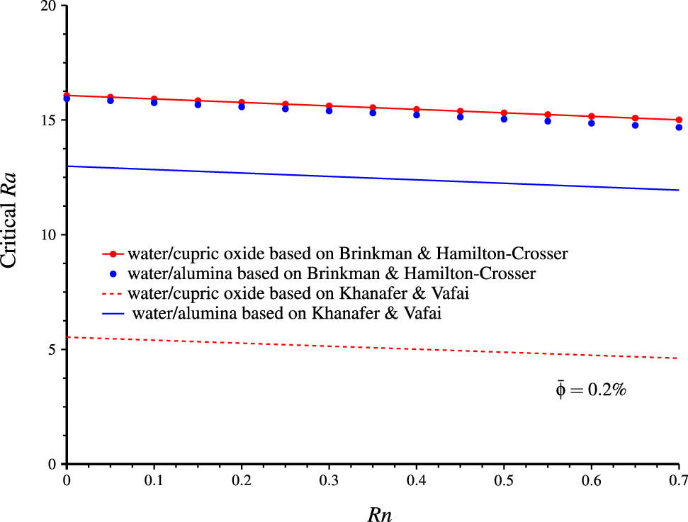
The relation between the concentration Rayleigh number and the critical thermal Rayleigh number for a DW/alumina nanofluid and a DW/cupric oxide nanofluid based on the model of Brinkman and Hamilton-Crosser and the model of Khanafer and Vafai.
Numerical results of the effect of the concentration Rayleigh number,
| Present | Nield and Kuznetsov [15] | ||||
|---|---|---|---|---|---|
| Rn | DW/alumina | DW/cupric oxide | Critical Ra | ||
| Critical Ra | Critical Ra | ||||
| KV | BHC | KV | BHC | ||
| 0.000 | 12.98769 | 15.93058 | 5.53184 | 16.07164 | 1707.1707 |
| 0.050 | 12.91351 | 15.84176 | 5.46652 | 15.99588 | 1629.1629 |
| 0.100 | 12.83913 | 15.75286 | 5.40119 | 15.92007 | 1549.1549 |
| 0.150 | 12.76478 | 15.66389 | 5.33578 | 15.84423 | 1468.1468 |
| 0.200 | 12.69042 | 15.57484 | 5.27036 | 15.76835 | 1386.1386 |
| 0.250 | 12.61593 | 15.48570 | 5.20487 | 15.69245 | 1302.1302 |
| 0.300 | 12.54144 | 15.39641 | 5.13938 | 15.61646 | 1216.1216 |
| 0.350 | 12.46688 | 15.30708 | 5.07375 | 15.54046 | 1128.1128 |
| 0.400 | 12.39228 | 15.21764 | 5.00813 | 15.46444 | 1038.1038 |
| 0.450 | 12.31759 | 15.12812 | 4.94246 | 15.38838 | 944.944 |
| 0.500 | 12.24287 | 15.03852 | 4.87674 | 15.31225 | 846.846 |
| 0.550 | 12.16811 | 14.94877 | 4.81095 | 15.23611 | 742.742 |
| 0.600 | 12.09326 | 14.85895 | 4.74519 | 15.15992 | 630.630 |
| 0.650 | 12.01841 | 14.76904 | 4.67929 | 15.08370 | 503.503 |
| 0.700 | 11.94345 | 14.67907 | 4.61337 | 15.00744 | 337.337 |
BHC: Brinkman and Hamilton-Crosser; KV: Khanafer and Vafai.
The numerical results of this model are compared with the numerical results of the same problem discussed by Nield and Kuznetsov [15]. Nield and Kuznetsov [15] discussed the same problem assuming that Brownian and thermophoresis diffusions are constants in the expression of the diffusive mass flux of the nanoparticles and that the material properties of nanofluid such as effective thermal conductivity and effective viscosity behave as parameters across the nanofluid layer. In their work, they did not produce any numerical results, so we had to solve their problem numerically and compare the results with the results obtained in our revised model. These results are listed in Table 1 where we compare the critical Rayleigh numbers obtained from Nield and Kuznetsov’s problem with the results obtained in this problem for the two types of nanofluids, DW/alumina oxide and DW/cupric oxide, and for the two models, Brinkman and Hamilton-Crosser and Khanafer and Vafai. The results indicate that using the revised model, which is more realistic, produce critical Rayleigh numbers which are less by one to two order of magnitude compared to the results obtained from the work of Nield and Kuznetsov [15]. In other words, our revised model is less stable. Finally, the numerical results obtained show that all critical eigenvalues were real valued, indicating that the mechanism of instability is by a non-oscillatory mode.
6 Conclusion
This study has proposed a revised model for the nanoparticle mass flux and used it to study the thermal instability of the Rayleigh-Benard convection for layers of DW/cupric oxide and DW/alumina nanofluids heated from below. The material properties of the nanofluids are allowed to depend on the local volume fraction of nanoparticles and are modelled by non-constant constitutive expressions developed by Kanafer and Vafai and Brinkman and Hamilton-Crosser. The analysis shows that the profile of the nanoparticle volume fraction of the steady-state solution is of exponential type. Stability results obtained show that
Based on the model of Khanafer and Vafai, the layer of DW/alumina nanofluid is more stable than the layer of DW/cupric oxide nanofluid if
Based on the model of Brinkman and Hamilton-Crosser, the layer of DW/cupric oxide nanofluid is more stable than the layer of DW/alumina nanofluid for all values of the nanoparticle volume fraction.
In general, the Brinkman and Hamilton-Crosser model is more stable than the Khanafer and Vafai model for both nanofluids.
The critical thermal Rayleigh number, Ra, decreases as the concentration Rayleigh number,
The critical Rayleigh numbers obtained for both nanofluids and for both models are compared with the results of Nield and Kuznetsov [15]. The results indicate that using the revised model, which is more realistic, produces critical Rayleigh numbers which are less by one to two order of magnitude compared to the results obtained from the work of Nield and Kuznetsov [15]. In other words, our revised model is less stable.
All the critical eigenvalues were real valued, indicating that the mechanism of instability is via a non-oscillatory mode.
-
Funding information: Authors state no funding involved.
-
Author contributions: Authors contributed equally to this work and approved its submission.
-
Conflict of interest: Authors state no conflict of interest.
-
Ethical approval: The conducted research is not related to either human or animal use.
-
Data availability statement: Data sharing is not applicable to this article as no datasets were generated or analyzed during the current study.
References
[1] H. Masuda , A. Ebata , K. Teramae , and N. Hishinuma , Alteration of thermal conductivity and viscosity of liquid by dispersing ultra-fine particles, Netsu. Bussei. 7 (1993), 227–233, https://doi.org/10.2963/jjtp.7.227. Search in Google Scholar
[2] S. Choi and J. Eastman , Enhancing thermal conductivity of fluids with nanoparticles , in: International Mechanical Engineering Congress & Exposition , ASME, San Francisco, 1995. Search in Google Scholar
[3] J. Eastman , S. Choi , S. Li , W. Yu , and L. Thompson , Anomalously increased effective thermal conductivities of ethylene glycol-based nanofluids containing copper nanoparticles, Appl. Phys. Lett. 78 (2001), 718–720, https://doi.org/10.1063/1.1341218 . 10.1063/1.1341218Search in Google Scholar
[4] S. Das , N. Putra , and W. Roetzel , Pool boiling characteristics of nano-fluids, Int. J. Heat Mass Trans. 46 (2003), no. 5, 851–862, https://doi.org/10.1016/S0017-9310(02)00348-4 . 10.1016/S0017-9310(02)00348-4Search in Google Scholar
[5] S. Jain , H. Patel , and S. Das , Brownian dynamic simulation for the prediction of effective thermal conductivity of nanofluid, J. Nanopart. Res. 11 (2009), 767, https://doi.org/10.1007/s11051-008-9454-4. Search in Google Scholar
[6] J. Kim , Y. Kang , and C. Choi , Analysis of convective instability and heat transfer characteristics of nanofluids, Phys. Fluids 16 (2004), no. 7, 2395–2401, https://doi.org/10.1063/1.1739247. Search in Google Scholar
[7] J. Buongiorno , Convective transport in nanofluids , J. Heat Trans. ASME 128 (2006), 240–250, https://doi.org/10.1115/1.2150834 . 10.1115/1.2150834Search in Google Scholar
[8] D. Tzou , Thermal instability of nanofluids in natural convection, Int. J. Heat Mass Trans. 51 (2008), 2967–2979, https://doi.org/10.1016/j.ijheatmasstransfer.2007.09.014. Search in Google Scholar
[9] D. Tzou , Instability of nanofluids in natural convection, ASME J. Heat Trans. 130 (2008), no. 7, 072401, https://doi.org/10.1115/1.2908427. Search in Google Scholar
[10] A. V. Kuznetsov and D. A. Nield , Thermal instability in a porous medium layer saturated by a nanofluid, Int. J. Heat Mass Trans. 52 (2009), 5796–5801, https://doi.org/10.1016/j.ijheatmasstransfer.2009.07.023. Search in Google Scholar
[11] D. A. Nield and A. V. Kuznetsov , The onset of convection in a horizontal nanofluid layer of finite depth, Eur. J. Mech. B/Fluids 29 (2010), 217–223, https://doi.org/10.1016/j.euromechflu.2010.02.003. Search in Google Scholar
[12] D. Yadav , G. S. Agrawal , and R. Bhargava , Thermal instability of rotating nanofluid layer, Int. J. Eng. Sci. 49 (2011), 1171–1184, https://doi.org/10.1016/j.asej.2015.05.005. Search in Google Scholar
[13] D. Yadav , R. Bhargava , and G. S. Agrawal , Thermal instability in a nanofluid layer with a vertical magnetic field, J. Eng. Math. 80 (2013), 147–164, https://doi.org/10.1007/s10665-012-9598-1. Search in Google Scholar
[14] A. Mahajan and M. Arora , Convection in rotating magnetic nanofluids, Appl. Math. Comput. 219 (2013), 3284–6296, https://doi.org/10.1016/j.amc.2012.12.012. Search in Google Scholar
[15] D. A. Nield and A. V. Kuznestov , The onset of convection in a horizontal nanofluid layer of finite depth: a revised model, Int. J. Heat Mass Trans. 77 (2014), 915–918, https://doi.org/10.1016/j.ijheatmasstransfer.2014.06.020. Search in Google Scholar
[16] S. Agarwal , P. Rana , and B. S. Bhadauria , Rayleigh-Benard convection in a nanofluid layer using a thermal nonequilibrium model, ASME J. Heat Trans. 136 (2014), no. 12, 122501, https://doi.org/10.1115/1.4028491. Search in Google Scholar
[17] D. Yadav , C. Kim , J. Lee , and H. H. Cho , Influence of magnetic field on the onset of nanofluid convection induced by purely internal heating, Comput. Fluids 121 (2015), 26–36, https://doi.org/10.1016/j.compfluid.2015.07.024. Search in Google Scholar
[18] S. Agarwal and P. Rana , Convective heat transport by longitudinal rolls in dilute nanoliquid layer of finite depth, Int. J. Therm. Sci. 108 (2016), 235–243, https://doi.org/10.1016/j.ijthermalsci.2016.05.013. Search in Google Scholar
[19] A. Abdullah and K. Lindsay , Marangoni convection in a layer of nanofluid, Int. J. Heat Mass Trans. 104 (2017), 693–702, https://doi.org/10.1016/j.ijheatmasstransfer.2016.08.099. Search in Google Scholar
[20] A. Abdullah , S. Althobaiti , and K. Lindsay , Marangoni convection in water-alumina nanofluids: Dependence on the nanoparticle size, Eur. J. Mech. B/Fluids 67 (2018), 259–268, https://doi.org/10.1016/j.euromechflu.2017.09.015. Search in Google Scholar
[21] G. Rana , P. Gautam , and H. Saxena , Electrohydrodynamic thermal instability in a walters (MODEL B) rotating nanofluid saturating a porous medium, J. Serb. Soc. Comput. Mech. 13 (2019), 19–35, https://doi.org/10.24874/jsscm.2019.13.02.03 . 10.24874/jsscm.2019.13.02.03Search in Google Scholar
[22] J. Ahuja and U. Gupta , Magneto convection in rotating nanofluid layer: Local thermal non-equilibrium model, J. Nanofluids 8 (2019), no. 2, 430–438, https://doi.org/10.1166/jon.2019.1585. Search in Google Scholar
[23] K. Khanafer and K. Vafai , A critical synthesis of thermophysical characteristics of nanofluids, Int. J. Heat Mass Trans. 4 (2011), 4410–4428, https://doi.org/10.1016/j.ijheatmasstransfer.2011.04.048. Search in Google Scholar
[24] H. C. Brinkman , The viscosity of concentrated suspensions and solutions, J. Chem. Phys. 20 (1952), no. 4, 571, https://doi.org/10.1063/1.1700493. Search in Google Scholar
[25] R. Hamilton and O. K. Crosser , Thermal conductivity of heterogeneous two-component systems, Ind. Eng. Chem. Fundamen. 1 (1962), no. 3, 187–191, https://doi.org/10.1021/i160003a005. Search in Google Scholar
© 2021 Ozwah S. Alharbi and Abdullah A. Abdullah, published by De Gruyter
This work is licensed under the Creative Commons Attribution 4.0 International License.
Articles in the same Issue
- Regular Articles
- Graded I-second submodules
- Corrigendum to the paper “Equivalence of the existence of best proximity points and best proximity pairs for cyclic and noncyclic nonexpansive mappings”
- Solving two-dimensional nonlinear fuzzy Volterra integral equations by homotopy analysis method
- Chandrasekhar quadratic and cubic integral equations via Volterra-Stieltjes quadratic integral equation
- On q-analogue of Janowski-type starlike functions with respect to symmetric points
- Inertial shrinking projection algorithm with self-adaptive step size for split generalized equilibrium and fixed point problems for a countable family of nonexpansive multivalued mappings
- On new stability results for composite functional equations in quasi-β-normed spaces
- Sampling and interpolation of cumulative distribution functions of Cantor sets in [0, 1]
- Meromorphic solutions of the (2 + 1)- and the (3 + 1)-dimensional BLMP equations and the (2 + 1)-dimensional KMN equation
- On the equivalence between weak BMO and the space of derivatives of the Zygmund class
- On some fixed point theorems for multivalued F-contractions in partial metric spaces
- On graded Jgr-classical 2-absorbing submodules of graded modules over graded commutative rings
- On almost e-ℐ-continuous functions
- Analytical properties of the two-variables Jacobi matrix polynomials with applications
- New soft separation axioms and fixed soft points with respect to total belong and total non-belong relations
- Pythagorean harmonic summability of Fourier series
- More on μ-semi-Lindelöf sets in μ-spaces
- Range-Kernel orthogonality and elementary operators on certain Banach spaces
- A Cauchy-type generalization of Flett's theorem
- A self-adaptive Tseng extragradient method for solving monotone variational inequality and fixed point problems in Banach spaces
- Robust numerical method for singularly perturbed differential equations with large delay
- Special Issue on Equilibrium Problems: Fixed-Point and Best Proximity-Point Approaches
- Strong convergence inertial projection algorithm with self-adaptive step size rule for pseudomonotone variational inequalities in Hilbert spaces
- Two strongly convergent self-adaptive iterative schemes for solving pseudo-monotone equilibrium problems with applications
- Some aspects of generalized Zbăganu and James constant in Banach spaces
- An iterative approximation of common solutions of split generalized vector mixed equilibrium problem and some certain optimization problems
- Generalized split null point of sum of monotone operators in Hilbert spaces
- Comparison of modified ADM and classical finite difference method for some third-order and fifth-order KdV equations
- Solving system of linear equations via bicomplex valued metric space
- Special Issue on Computational and Theoretical Studies of free Boundary Problems and their Applications
- Dynamical study of Lyapunov exponents for Hide’s coupled dynamo model
- A statistical study of COVID-19 pandemic in Egypt
- Global existence and dynamic structure of solutions for damped wave equation involving the fractional Laplacian
- New class of operators where the distance between the identity operator and the generalized Jordan ∗-derivation range is maximal
- Some results on generalized finite operators and range kernel orthogonality in Hilbert spaces
- Structures of spinors fiber bundles with special relativity of Dirac operator using the Clifford algebra
- A new iteration method for the solution of third-order BVP via Green's function
- Numerical treatment of the generalized time-fractional Huxley-Burgers’ equation and its stability examination
- L ∞-error estimates of a finite element method for Hamilton-Jacobi-Bellman equations with nonlinear source terms with mixed boundary condition
- On shrinkage estimators improving the positive part of James-Stein estimator
- A revised model for the effect of nanoparticle mass flux on the thermal instability of a nanofluid layer
- On convergence of explicit finite volume scheme for one-dimensional three-component two-phase flow model in porous media
- An adjusted Grubbs' and generalized extreme studentized deviation
- Existence and uniqueness of the weak solution for Keller-Segel model coupled with Boussinesq equations
- Special Issue on Advanced Numerical Methods and Algorithms in Computational Physics
- Stability analysis of fractional order SEIR model for malaria disease in Khyber Pakhtunkhwa