An adjusted Grubbs' and generalized extreme studentized deviation
-
Mufda Jameel Alrawashdeh


Abstract
Detecting outlier data is an interesting subject in the statistical field. Grubbs’ test is one of the common detection methods of outlier observation at univariate data sets. This approach is based on the mean and standard deviation of univariate data, and hence, these data are highly affected by the presence of outliers. An improvement for Grubbs’ test is proposed in this paper to increase the power of detecting data.
1 Introduction
The presence of outliers (extreme points) is the main problem that destroys analysis results. Therefore, studying outlier detection methods is crucial in statistics. These detection methods have a strong impact in estimating data analysis results and might be more interesting than the other data in some cases. Thus, outlier detection is the observation with large deviations from the other observations. This type of observation may be defined as observation generated by different mechanism reasons according to [1]. In the last few decades, many studies have introduced methods to detect the outliers for multivariate and univariate data. Examples of these methods include
Most of the statistical tests for detecting the presence of outliers handle one outlier at once. The outlier is removed from the data set when its measurement is located and the process is repeated until all suspected outliers are detected. One of the common testing methods used for univariate data to detect the presence of outlier data is Grubbs’ test, which was introduced in 1950 [10] and extended by the same author in 1969 [11] and 1972 [12]. Grubbs’ test is known in different names, such as maximum normed residual test or extreme studentized deviation (ESD) test. The mean, standard deviation, and the tabulated criterion are used to apply Grubbs’ test, and the tabulated value for critical value is compared for the level of significance.
Grubbs’ test has been applied in different studies for the last few decades to detect outliers. Previous studies [13,14, 15,16,17], applied this test to detect the outlier observation. The advantages and disadvantages of Grubbs’ test have been studies over the last few decades, which helps to improve the performance of this test. Rosner [13] compared Grubbs’ test and studentized range methods and found that Grubbs’ test performed efficiently and was similar to the kurtosis and R-statistic method.
Grubbs’ and the generalized ESD tests require mean and standard deviation for their application. Both tests are highly affected by the presence of outlier data, thus yielding accurate results.
Rosner [18] introduced the generalized ESD to test the presence of one or more outliers in a univariate data set that follows an approximately normal distribution. This test requires an upper bound of the suspected number of existing outliers. However, the generalized ESD remained inefficient for sample sizes less than 25. Another improvement was introduced by Brant [19], who reported the combination of ESD rules and box-plot. This combination revealed that the selection of a suitable ESD has comparable performance to box-plot rules in non-Gaussian situations and superior to the pure Gaussian case. Grubbs’ test also failed to detect outliers because the sample mean and standard deviation are highly affected by the presence of outliers [20]. The generalized ESD and Grubbs’ tests have been applied in different studies, demonstrating a robust equicorrelation effect of observation and a constant significant level [21]. The complete solution of the problem is derived, wherein the characteristics of Grubbs’ test are invariant, given a dispersion matrix if and only if it has established Baldessari structure [22]. Grubbs’ test is applied to a new transformed data set. The new technique improves the capability of outlier detection, wherein the results show that Grubbs’ test can identify the outliers at a significant level of 0.01, after data transformation; notably, the observations are identified at significant level 0.05, before the transformation [23]. Four types of estimation
The previous literature showed that all researchers used mean and standard deviation of the data for Grubbs’ test. However, modification of the test formula by replacing the test parameters is not attempted due to their substantial sensitivity to outlier observation. One of the most robust parameters for outliers is the median of data. Thus, the mean is replaced by the median and the result showed increased efficacy of the outlier detection observation. Stahel [29] and Donoho [30], revealed that the median is used to adjust box-plots, where the outlyingness of a univariate point
where
This study aims to introduce a method to replace the mean of data by its median for application in Grubbs’ test. Furthermore, the replacement of mean by the data median increases the capability of overcoming the presence of outliers due to the substantial sensitivity of the mean to outlier observations. Therefore, the application of the mean in the test may be influenced by the outliers, such as the data presented in Figure 1.
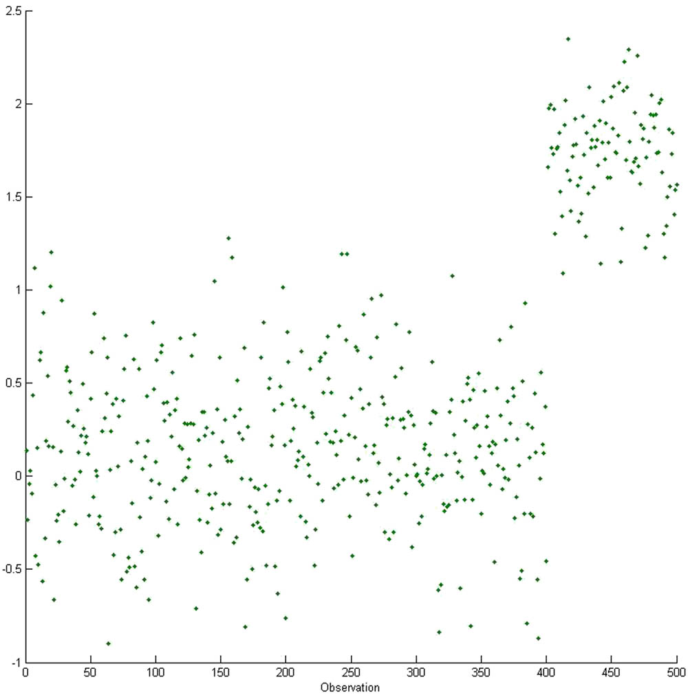
Spread observation example of a group of data.
2 Grubbs’ and generalized ESD test of detecting outliers
2.1 Generalized ESD test
Previous study [18] applied ESD test to detect the presence of one or more outliers at univariate data that follows an approximately normal distribution. The generalized ESD test required only a specified upper bound
First, the maximum value of
The significance level and critical value corresponding to the test statistics are calculated
where
2.2 Grubbs’ test
Grubbs’ test [10] is used to distinguish and detect the presence of outlier observations, whose distribution is approximately Gaussian. As previously mentioned, Grubbs’ test was introduced in 1950 and extended by the same author in 1969 and then 1972. This test is also known as the maximum normed residual test or ESD test and, defined as follows:
where
Test whether the minimum value is an outlier
Test whether the maximum value is an outlier
where
3 Robust tests
The main idea of robust generalized ESD and Grubbs’ tests involves replacing the mean of the data set by its median. All previous researchers used the original procedure of Grubbs’ test for detecting the outlier observations. However, this study applied both tests as the original ones with the data set median instead of using its mean.
3.1 Generalized ESD
The mean of the data set is replaced by the median to strengthen the generalized ESD test, and the hypothesis test is the same as in 2.1. The test statistic is computed as follows:
3.2 Grubbs’ test
The new Grubbs’ test is defined as follows:
where
Arrange the observations
Calculate the Grubbs’ test parameters and the
Obtain the
Decision making.
4 Simulation study
Generalized ESD and Grubbs’ test will be applied for univariate generated data from the original and new version. The data should be univariate and the generated data should be normally distributed as follows:
where
The data are constructed for single and multiple outliers. The test has also been applied 1,000 times; the data are generated each time and both tests are applied. The tests are constructed in two versions: one version is used with the mean of the data and the second version is applied with the median of data instead of using their mean. However, the two versions have been applied for different levels of alpha values as follows:
4.1 Grubbs’ test result
The univariate data are generated in this simulation study, followed by the normal distribution. Figure 2 presents the generated data set with one unusual observation that is used for this test. Table 1 shows the result of 1,000 replications for Grubbs’ test. The test has been applied for original and new versions of Grubbs’ test. Table 1 reveals the number of outliers detected, wherein the number of outliers detected by Grubbs’ test using the median is more than that of the original test. The difference between the two versions is minimal, the differences are 4, 1, and 18 outliers at
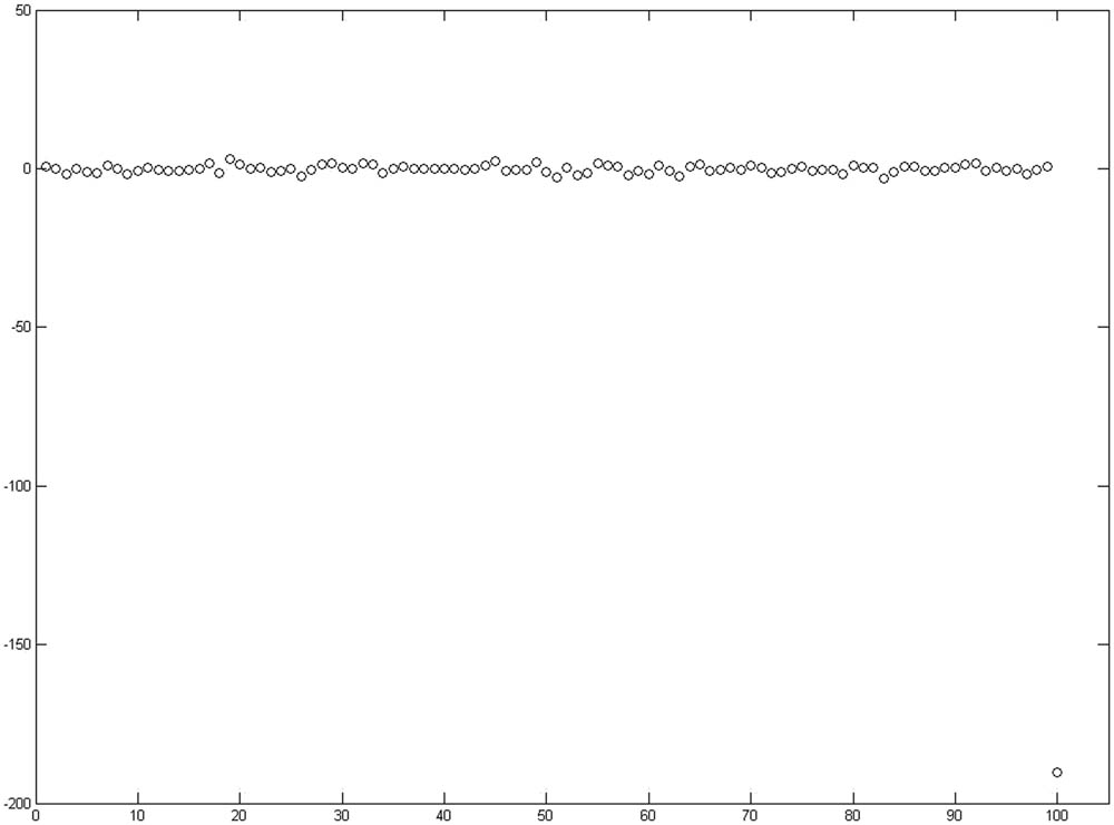
Example of the normal data containing one outlier observation used for Grubbs’ test simulation.
Two types of parameters and the
| Type of parameter | Alpha value | Number outliers | Average of all the
|
|---|---|---|---|
| Mean | 0.01 | 441 | 5.3454930514195 |
| Median | 0.01 | 445 | 5.37140145603596 |
| Mean | 0.05 | 534 | 4.87943251409262 |
| Median | 0.05 | 535 | 4.90527097577631 |
| Mean | 0.1 | 591 | 4.54648039744501 |
| Median | 0.1 | 607 | 4.52467760964745 |
Sample of ten replications of Grubbs’ test out of 1,000 replications
| Mean | Median | Mean | Median | Mean | Median |
|---|---|---|---|---|---|
|
|
|
|
|
|
|
| 4.99791548 | 5.00746574 | 4.99791548 | 5.00746574 | 4.99791548 | 5.0074657 |
| 4.72022356 | 4.67885211 | 4.72022356 | 4.6788521 | 4.72022356 | 4.6788521 |
| 3.13544118 | 3.19163785 | 7.89846662 | 8.00485689 | 7.89846661 | 8.00485689 |
| 4.29169032 | 4.31836035 | 4.29169032 | 4.31836035 | 4.29169032 | 4.31836035 |
| 6.39971758 | 6.56332671 | 6.39971758 | 6.56332671 | 6.39971758 | 6.56332679 |
| 8.72933862 | 8.79539702 | 8.72933862 | 8.79539702 | 8.70933865 | 8.79539702 |
| 4.93489331 | 5.00121965 | 4.93489332 | 5.00121966 | 4.98689331 | 5.00121965 |
| 5.42234464 | 5.43638784 | 5.42234465 | 5.43638784 | 5.42254465 | 5.43638784 |
| 3.29664302 | 3.28492568 | 3.29664302 | 3.28492568 | 4.37851618 | 4.4836639 |
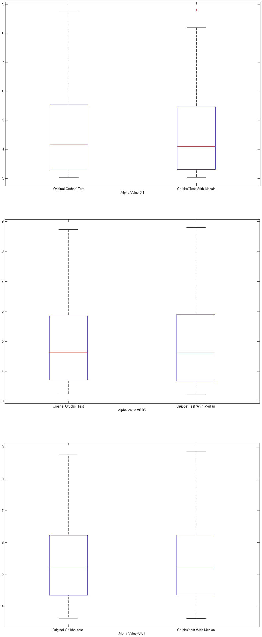
The box-plot for original and new Grubbs’ test for three
5 Generalized ESD test result
Figure 4 is an example of group of data that we use through the simulation study for generalized ESD test. At the generalized ESD procedure we run
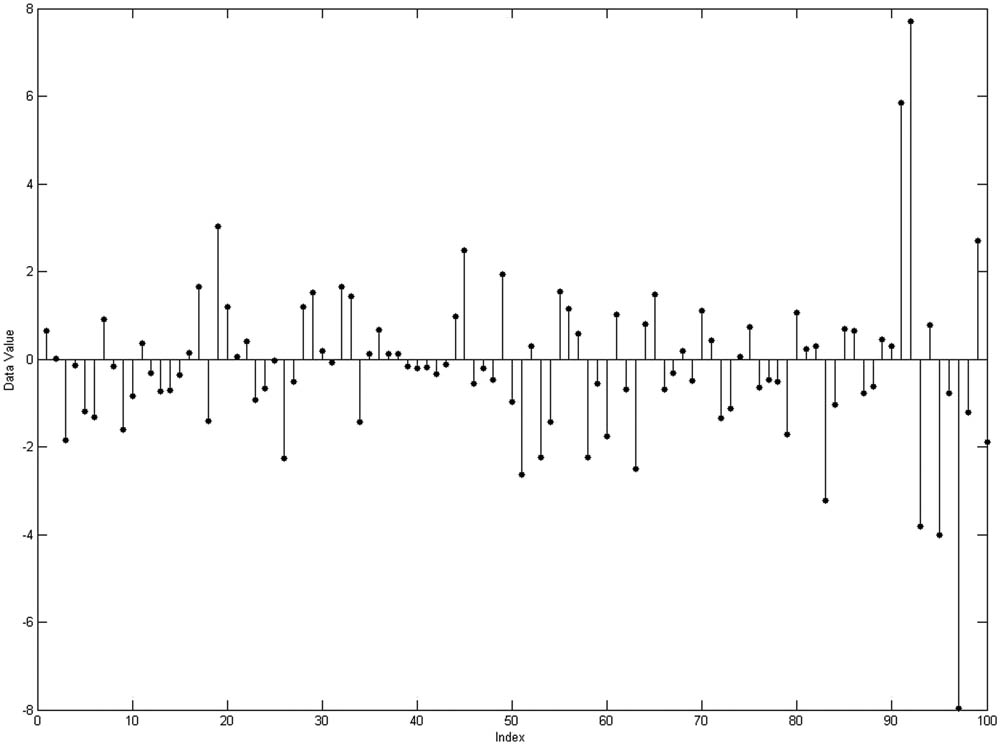
Spread observation example of a group of data as example of generalized ESD data.
Sample of ten maximum values of rth for 1,000 replications of generalized ESD test
| Mean | Median | Mean | Median | Mean | Median |
|---|---|---|---|---|---|
| 5.300430002 | 5.203295069 | 5.71472549 | 5.570904725 | 5.35591713 | 5.310421837 |
| 4.070808367 | 4.117045592 | 4.150222854 | 4.205011857 | 4.39602947 | 4.279707365 |
| 6.169652668 | 6.172189401 | 3.735935686 | 3.640060263 | 3.923644425 | 4.028206728 |
| 4.759616896 | 4.678920536 | 3.935229529 | 3.871017171 | 3.397269384 | 3.334165472 |
| 3.829540283 | 3.985780779 | 4.081865981 | 4.119122537 | 3.888871123 | 3.846694817 |
| 3.573970163 | 3.543340603 | 3.111995699 | 2.896459924 | 4.470188945 | 4.382753211 |
| 4.101755091 | 4.115631057 | 2.645034796 | 2.639705743 | 2.868091054 | 2.675174872 |
| 2.495916551 | 2.542589952 | 3.857517887 | 3.801118877 | 2.582812931 | 2.593586935 |
| 2.262514987 | 2.436528915 | 2.101608211 | 2.176991513 | 2.876891594 | 2.847042216 |
| 2.580364591 | 2.552446223 | 2.256054084 | 2.265538408 | 2.082631391 | 2.182874679 |
| 2.779804583 | 2.767503326 | 2.482727728 | 2.470165789 | 2.155632263 | 2.077781431 |
| 2.070126694 | 2.015338046 | 2.725057463 | 2.71870878 | 2.438857826 | 2.439918636 |
| 2.149246808 | 1.991473785 | 2.015162636 | 1.973719327 | 2.054947758 | 2.043116464 |
| 2.458953457 | 2.444317153 | 5.498782864 | 5.444205319 | 5.271140234 | 5.235878777 |
| 4.70562353 | 4.69233363 | 5.200478464 | 5.057225327 | 4.779359114 | 4.757353968 |
| 5.462103129 | 5.478784101 | 4.627314023 | 4.663037715 | 4.673352835 | 4.565877198 |
| 4.650019999 | 4.623431136 | 3.771984071 | 3.833171563 | 4.048898887 | 3.969862562 |
| 3.788732048 | 3.716590666 | 4.490024378 | 4.470267213 | 3.811299799 | 3.78273964 |
| 3.594092799 | 3.62416543 | 3.882681257 | 3.842249739 | 2.192316979 | 2.217823645 |
| 3.955830893 | 3.983784999 | 3.803369769 | 3.777382906 | 3.085307907 | 3.078092184 |
| 2.203772269 | 2.176379838 | 3.147560491 | 3.051442616 | 3.963833845 | 4.006183014 |
| 2.880953678 | 2.900266821 | 2.170171417 | 2.217626525 | 2.806251077 | 2.724680092 |
| 3.619055938 | 3.518439247 | 2.70586475 | 2.654562996 | 2.193549521 | 2.204403805 |
| 2.916851336 | 2.7757971 | 2.458136407 | 2.368844298 | 2.454629576 | 2.479240315 |
| 2.137211278 | 2.19613043 | 2.786413065 | 2.887815709 | 2.421693815 | 2.351646994 |
| 2.486797174 | 2.504792535 | 2.180372308 | 2.250388542 | 2.620009583 | 2.500475795 |
| 2.123304242 | 2.173614836 | 2.522668822 | 2.482058356 | 5.502486098 | 5.440427526 |
| 6.303581351 | 6.215067768 | 5.817524369 | 5.8740713 | 5.331936524 | 5.18935738 |
| 4.558058988 | 4.674861556 | 4.022272734 | 3.849290853 | 3.802895094 | 3.644670821 |
| 5.570856767 | 5.560783171 | 5.271914513 | 5.230373984 | 4.522718631 | 4.383705974 |
| 6.600997557 | 6.552098733 | 4.558446943 | 4.548234141 | 4.890267956 | 4.780835832 |
| 4.504954764 | 4.520065448 | 4.292304867 | 4.255242213 | 3.629808288 | 3.55591935 |
| 3.667243481 | 3.600331585 | 2.651361851 | 2.647898658 | 2.475512044 | 2.498564178 |
| 2.03241704 | 2.211162707 | 2.189843656 | 2.35469121 | 2.677959848 | 2.812773134 |
| 3.051158696 | 3.016947219 | 2.689065776 | 2.709583109 | 2.521269187 | 2.46535682 |
| 2.923271844 | 2.937883779 | 2.575528 | 2.537898903 | 2.552266775 | 2.525055908 |
| 2.223281959 | 2.242155817 | 2.445203364 | 2.42060523 | 2.5598113 | 2.510908888 |
| 2.047841001 | 2.005440106 | 2.062315498 | 2.255860165 | 2.01163477 | 2.202250804 |
| 2.241679653 | 2.213810188 | 2.468437007 | 2.46500754 | 2.511954764 | 2.47297268 |
| 2.127573744 | 2.089987775 | 2.310108944 | 2.291089551 | 2.5177393 | 2.488370115 |
Average of sample of all
|
|
|
|
|
|
|
|
|
|
|
|
|---|---|---|---|---|---|---|---|---|---|---|
|
|
0.77967 | 0.79529 | 0.81124 | 0.8075 | 0.73484 | 0.78023 | 0.79627 | 0.80559 | 0.76435 | 0.80517 |
|
|
0.77395 | 0.79697 | 0.81132 | 0.79130 | 0.73262 | 0.77845 | 0.78228 | 0.79894 | 0.7616 | 0.80052 |
|
|
0.7673 | 0.79705 | 0.80752 | 0.78165 | 0.72952 | 0.77526 | 0.773 | 0.79534 | 0.75770 | 0.79879 |
|
|
0.75989 | 0.79037 | 0.80414 | 0.77124 | 0.72543 | 0.77370 | 0.76795 | 0.76086 | 0.74969 | 0.7793 |
|
|
0.75361 | 0.77856 | 0.79324 | 0.73330 | 0.72156 | 0.77267 | 0.753089 | 0.72266 | 0.73878 | 0.76595 |
|
|
0.74139 | 0.76805 | 0.72740 | 0.6973 | 0.7170 | 0.7709 | 0.71190 | 0.69897 | 0.7258 | 0.73744 |
|
|
0.73275 | 0.72698 | 0.69824 | 0.67704 | 0.69032 | 0.70193 | 0.69254 | 0.68506 | 0.69328 | 0.68397 |
|
|
0.68573 | 0.69549 | 0.64749 | 0.6559 | 0.68060 | 0.65674 | 0.67067 | 0.65729 | 0.67543 | 0.54072 |
|
|
0.63437 | 0.66209 | 0.62416 | 0.54004 | 0.6615 | 0.61387 | 0.58663 | 0.61258 | 0.62984 | 0.49989 |
|
|
0.61014 | 0.59628 | 0.55033 | 0.50638 | 0.63309 | 0.55083 | 0.54245 | 0.57806 | 0.57951 | 0.46280 |
Average of sample of all
|
|
|
|
|
|
|
|
|
|
|
|
|---|---|---|---|---|---|---|---|---|---|---|
|
|
0.78108 | 0.82073 | 0.81796 | 0.80781 | 0.73548 | 0.78290 | 0.80106 | 0.80650 | 0.76850 | 0.79133 |
|
|
0.77403 | 0.82063 | 0.81541 | 0.79138 | 0.73261 | 0.78030 | 0.78815 | 0.80158 | 0.76269 | 0.7852 |
|
|
0.76762 | 0.81219 | 0.80985 | 0.78192 | 0.72980 | 0.77996 | 0.78341 | 0.79826 | 0.75819 | 0.78013 |
|
|
0.76022 | 0.80191 | 0.80619 | 0.77193 | 0.72611 | 0.77665 | 0.77304 | 0.76417 | 0.75151 | 0.77019 |
|
|
0.75395 | 0.79511 | 0.79446 | 0.73464 | 0.72156 | 0.77421 | 0.76050 | 0.72779 | 0.73915 | 0.7557 |
|
|
0.74188 | 0.78524 | 0.73214 | 0.70046 | 0.71713 | 0.77114 | 0.72310 | 0.70423 | 0.72593 | 0.73347 |
|
|
0.73474 | 0.73621 | 0.69919 | 0.67809 | 0.69210 | 0.70234 | 0.69811 | 0.68588 | 0.69543 | 0.70245 |
|
|
0.68581 | 0.70112 | 0.65197 | 0.65853 | 0.68516 | 0.65755 | 0.67187 | 0.65990 | 0.67988 | 0.67242 |
|
|
0.63678 | 0.66413 | 0.63067 | 0.54004 | 0.67089 | 0.61432 | 0.58664 | 0.61277 | 0.63766 | 0.62154 |
|
|
0.61021 | 0.60396 | 0.56076 | 0.50914 | 0.63527 | 0.55353 | 0.54488 | 0.57860 | 0.59164 | 0.57644 |
6 Conclusion
In this paper, we have proposed an outlier detection method for univariate data. The procedure is based on the Grubbs’ and generalized ESD tests with its median instead of the data mean used, whereas the new method that is considered as improver of the classical Grubbs’ and generalized ESD used the mean of data. The mean of data is very sensitive to the presence of outlier observation in data set and the median is more robust and more resistant to outlier. Simulation has illustrated that a new version of both tests, performance is robust compared to the classical Grubbs’ and generalized tests.
-
Funding information: The author states no funding involved.
-
Conflict of interest: The author states no conflict of interest.
References
[1] V. Barnett and T. Lewis, Outliers in Statistical Data, Wiley Series in Probability and Statistics, New York, 1984. Search in Google Scholar
[2] F. Mosteller and J. W. Tukey, Data Analysis and Regression: A Second Course in Statistics, Addison-Wesley Ser. Math., 1977. Search in Google Scholar
[3] M. Hubert and E. Vandervieren, An adjusted boxplot for skewed distributions, Comput. Statist. Data Anal. 52 (2004), 5186–5201. 10.1016/j.csda.2007.11.008Search in Google Scholar
[4] P. J. Rousseeuw and K. V. Driessen, A fast algorithm for the minimum covariance determinant estimator, Technometrics 41 (1999), 212–223. 10.1080/00401706.1999.10485670Search in Google Scholar
[5] P. M. Hubert, P. J. Rousseeuw, D. Vanpaemel, and T. Verdonck, The DetS and DetMM estimators for multivariate location and scatter, Comput. Statist. Data Anal. 81 (2015), 64–75. 10.1016/j.csda.2014.07.013Search in Google Scholar
[6] N. Balakrishnan, E. Castilla, N. Martín, and L. Pardo, Robust estimators and test statistics for one-shot device testing under the exponential distribution, IEEE Trans. Info. Theor. 65 (2019), 3080–3096. 10.1109/TIT.2019.2903244Search in Google Scholar
[7] P. Duchesne and R. Roy, Robust tests for independence of two time series, Statist. Sinica 13 (2003), 827–852. Search in Google Scholar
[8] N. Cvejic and T. Seppanen, Robust audio watermarking in wavelet domain using frequency hopping and patchwork method, Statist. Sinica 1 (2003), 251–255. 10.1109/ISPA.2003.1296903Search in Google Scholar
[9] A. M. Bianco and M. Martínez, Robust testing in the logistic regression model, Statist. Sinica 53 (2009), 4095–4105. 10.1016/j.csda.2009.04.015Search in Google Scholar
[10] E. G. Frank, Sample criteria for testing outlying observations, Inst. Math. Stat. 21 (1950), 27–58. 10.1214/aoms/1177729885Search in Google Scholar
[11] E. G. Frank, Procedures for detecting outlying observations in samples, Technometrics 11 (1969), 1–21. 10.1080/00401706.1969.10490657Search in Google Scholar
[12] E. G. Frank and B. Glenn, Extension of sample sizes and percentage points for significance tests of outlying observations, Technometrics 14 (1972), 847–854. 10.1080/00401706.1972.10488981Search in Google Scholar
[13] B. Rosner, On the detection of many outliers, Technometrics 17 (1975), 221–227. 10.2307/1268354Search in Google Scholar
[14] M. K. Solak, Detection of Multiple Outliers in Univariate Data Sets, Schering, Wedding, Berlin, 2009. Search in Google Scholar
[15] M. Thompson and P. J. Lowthian, Notes on statistics and data quality for analytical chemists, World Scientific Lecture Notes in Economics, Imperial College Press, London, 2011. 10.1142/p739Search in Google Scholar
[16] R. B. Jain, A recursive version of Grubbs’ test for detecting multiple outliers in environmental and chemical data, Clin. Biochem. 43 (2010), 1030–1033. 10.1016/j.clinbiochem.2010.04.071Search in Google Scholar PubMed
[17] B. M. Colosimo, R. Pan, and E. Castillo, A sequential Markov chain Monte Carlo approach to set-up adjustment of a process over a set of lots, J. Appl. Stat. 5 (2004), 499–520. 10.1080/02664760410001681765Search in Google Scholar
[18] B. Rosner, Percentage points for a generalized ESD many-outlier procedure, Technometrics 25 (1983), 165–172.10.1080/00401706.1983.10487848Search in Google Scholar
[19] R. Brant, Comparing classical and resistant outlier rules, J. Amer. Statist. Assoc. 85 (1990), 1083–1090. 10.1080/01621459.1990.10474979Search in Google Scholar
[20] L. Zhang, P. Xu, J. Xu, S. Wu, G. Han, and D. Xu, Conflict Analysis of Multi-Source SST Distribution, Springer, Berlin, Heidelberg, 2010. Search in Google Scholar
[21] M. Srivastava, Effect of equicorrelation in detecting a spurious observation, Canad. J. Statist. 8 (1980), 249–251. 10.2307/3315236Search in Google Scholar
[22] J. K. Baksalary and S. Puntanen, A complete solution to the problem of robustness of Grubbs’ test, Canad. J. Statist. 18 (1990), 285–287. 10.2307/3315459Search in Google Scholar
[23] B. Y. Lemeshko and B. S. Lemeshko, Extending the application of Grubbs-type tests in rejecting anomalous measurements, Meas. Tech. 48 (2005), 536–547. 10.1007/s11018-005-0179-9Search in Google Scholar
[24] D. Ekezie and I. A. Jeoma, Statistical analysis/methods of detecting outliers in a univariate data in a regression analysis model, Int. J. Edu. Res. 1 (2013), 1–25. Search in Google Scholar
[25] M. Urvoy and F. Autrusseau, Application of Grubbs’ test for outliers to the detection of watermarks, Proceedings of the 2nd ACM Workshop on Information Hiding and Multimedia Security, 2014. 10.1145/2600918.2600931Search in Google Scholar
[26] R. Paul Sudhir and Y. Fung Karen, Features and performance of some outlier detection methods, Technometrics 33 (1981), 339–348. 10.1080/00401706.1991.10484839Search in Google Scholar
[27] G. Barbato, E. Barini, G. Genta, and R. Levi, A generalized extreme studentized residual multiple-outlier-detection procedure in linear regression, J. Appl. Stat. 38 (2011), 2133–2149. 10.1080/02664763.2010.545119Search in Google Scholar
[28] K. Manoj and S. Kannan, Comparison of methods for detecting outliers, Int. J. Sci. Eng. Res. 4 (2013), 709–714. Search in Google Scholar
[29] A. Stahel, Robuste schätzungen: infinitesimale optimalität und schätzungen von kovarianzmatrizen, Ph.D. thesis, ETH Zürich, 1981. Search in Google Scholar
[30] D. L. Donoho, Breakdown properties of multivariate location estimators, Ann. Statist. 20 (1992), 1803–1827. 10.1214/aos/1176348890Search in Google Scholar
© 2021 Mufda Jameel Alrawashdeh, published by De Gruyter
This work is licensed under the Creative Commons Attribution 4.0 International License.
Articles in the same Issue
- Regular Articles
- Graded I-second submodules
- Corrigendum to the paper “Equivalence of the existence of best proximity points and best proximity pairs for cyclic and noncyclic nonexpansive mappings”
- Solving two-dimensional nonlinear fuzzy Volterra integral equations by homotopy analysis method
- Chandrasekhar quadratic and cubic integral equations via Volterra-Stieltjes quadratic integral equation
- On q-analogue of Janowski-type starlike functions with respect to symmetric points
- Inertial shrinking projection algorithm with self-adaptive step size for split generalized equilibrium and fixed point problems for a countable family of nonexpansive multivalued mappings
- On new stability results for composite functional equations in quasi-β-normed spaces
- Sampling and interpolation of cumulative distribution functions of Cantor sets in [0, 1]
- Meromorphic solutions of the (2 + 1)- and the (3 + 1)-dimensional BLMP equations and the (2 + 1)-dimensional KMN equation
- On the equivalence between weak BMO and the space of derivatives of the Zygmund class
- On some fixed point theorems for multivalued F-contractions in partial metric spaces
- On graded Jgr-classical 2-absorbing submodules of graded modules over graded commutative rings
- On almost e-ℐ-continuous functions
- Analytical properties of the two-variables Jacobi matrix polynomials with applications
- New soft separation axioms and fixed soft points with respect to total belong and total non-belong relations
- Pythagorean harmonic summability of Fourier series
- More on μ-semi-Lindelöf sets in μ-spaces
- Range-Kernel orthogonality and elementary operators on certain Banach spaces
- A Cauchy-type generalization of Flett's theorem
- A self-adaptive Tseng extragradient method for solving monotone variational inequality and fixed point problems in Banach spaces
- Robust numerical method for singularly perturbed differential equations with large delay
- Special Issue on Equilibrium Problems: Fixed-Point and Best Proximity-Point Approaches
- Strong convergence inertial projection algorithm with self-adaptive step size rule for pseudomonotone variational inequalities in Hilbert spaces
- Two strongly convergent self-adaptive iterative schemes for solving pseudo-monotone equilibrium problems with applications
- Some aspects of generalized Zbăganu and James constant in Banach spaces
- An iterative approximation of common solutions of split generalized vector mixed equilibrium problem and some certain optimization problems
- Generalized split null point of sum of monotone operators in Hilbert spaces
- Comparison of modified ADM and classical finite difference method for some third-order and fifth-order KdV equations
- Solving system of linear equations via bicomplex valued metric space
- Special Issue on Computational and Theoretical Studies of free Boundary Problems and their Applications
- Dynamical study of Lyapunov exponents for Hide’s coupled dynamo model
- A statistical study of COVID-19 pandemic in Egypt
- Global existence and dynamic structure of solutions for damped wave equation involving the fractional Laplacian
- New class of operators where the distance between the identity operator and the generalized Jordan ∗-derivation range is maximal
- Some results on generalized finite operators and range kernel orthogonality in Hilbert spaces
- Structures of spinors fiber bundles with special relativity of Dirac operator using the Clifford algebra
- A new iteration method for the solution of third-order BVP via Green's function
- Numerical treatment of the generalized time-fractional Huxley-Burgers’ equation and its stability examination
- L ∞-error estimates of a finite element method for Hamilton-Jacobi-Bellman equations with nonlinear source terms with mixed boundary condition
- On shrinkage estimators improving the positive part of James-Stein estimator
- A revised model for the effect of nanoparticle mass flux on the thermal instability of a nanofluid layer
- On convergence of explicit finite volume scheme for one-dimensional three-component two-phase flow model in porous media
- An adjusted Grubbs' and generalized extreme studentized deviation
- Existence and uniqueness of the weak solution for Keller-Segel model coupled with Boussinesq equations
- Special Issue on Advanced Numerical Methods and Algorithms in Computational Physics
- Stability analysis of fractional order SEIR model for malaria disease in Khyber Pakhtunkhwa