Linearity assessment: deviation from linearity and residual of linear regression approaches
-
Chun Yee Lim
 ,
Tze Ping Loh
,
Tze Ping Loh
 ,
Chung Shun Ho
,
Chung Shun Ho

Abstract
In this computer simulation study, we examine four different statistical approaches of linearity assessment, including two variants of deviation from linearity (individual (IDL) and averaged (AD)), along with detection capabilities of residuals of linear regression (individual and averaged). From the results of the simulation, the following broad suggestions are provided to laboratory practitioners when performing linearity assessment. A high imprecision can challenge linearity investigations by producing a high false positive rate or low power of detection. Therefore, the imprecision of the measurement procedure should be considered when interpreting linearity assessment results. In the presence of high imprecision, the results of linearity assessment should be interpreted with caution. Different linearity assessment approaches examined in this study performed well under different analytical scenarios. For optimal outcomes, a considered and tailored study design should be implemented. With the exception of specific scenarios, both ADL and IDL methods were suboptimal for the assessment of linearity compared. When imprecision is low (3 %), averaged residual of linear regression with triplicate measurements and a non-linearity acceptance limit of 5 % produces <5 % false positive rates and a high power for detection of non-linearity of >70 % across different types and degrees of non-linearity. Detection of departures from linearity are difficult to identify in practice and enhanced methods of detection need development.
Introduction
Linearity assessment is an evaluation of the linear relationship between the measured (observed) values of a measurand and the true (assigned) values in a series of samples [1, 2]. There is guidance on the requirements to perform linearity assessment as part of pre-implementation method evaluation and periodic (e.g. six monthly or when analytical issue is suspected) reassessment of linearity assessment. Ideally, linearity assessments should be performed using commutable materials (e.g. residual patient samples) to ensure findings are translatable to results from patient samples. Non-linearity is generally sub-optimally detected or monitored by internal quality control procedures since they examines limited number of samples/concentrations. At the same time, the presence of significant non-linearity may be associated with poorer proficiency testing performance, likely depending on the concentration of the proficiency materials [3, 4].
Several approaches have been described to assess linearity in the clinical laboratory [1, 5]. Early assessment procedures for linearity were based on visual assessment of manually graphed points and straight line of best fit characterised. However, this approach is highly subjective in nature and not readily reproducible. More recently, software developments combined with formal statistical assessment have improved the objectivity and reproducibility of such assessments [6], [7], [8], [9].
In this computer simulation study, in recognition of the varying statistical approaches, study designs and laboratory conditions we examine four different statistical approaches of linearity assessment, including two variants of deviation from linearity, along with detection capabilities of residuals of linear regression. From this, we aim to provide the performance characteristics of these statistical approaches and study designs.
Methods
To evaluate linearity, samples with equidistant concentrations spanning an arbitrary analytical measurement range are simulated. The results of the simulated measurement are fitted with a straight line (linear regression), as well as quadratic and cubic lines (quadratic and cubic regressions) as defined below (Figure 1A):
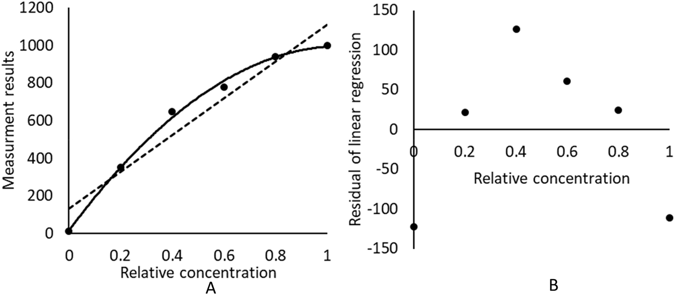
Illustration of statistical model fitting for measurement results in linearity assessment. (A) Fitting linear and nonlinear models to measurement results; (B) residuals of linear regression. Note curved nature of residuals indicating non-linearity.
Approaches to linearity assessment studied
Four approaches to linearity are assessed: (1) deviation from linearity – individual (IDL); (2) deviation from linearity – average (ADL); (3) regression residual – individual; and (4) regression residual – average.
Individual deviation from linearity (IDL)
Alternatively, instead of averaging the differences across all concentration points, the individual deviation from linearity, which is defined as the absolute difference between the linear and nonlinear fits (quadratic and cubic) at each concentration, it can be examined:
The IDL at each concentration was then compared against an a priori defined linearity acceptance limit using the average of the replicate measurements (if performed). When any of the IDLs exceeded the specified limit, non-linearity was considered detected.
Average deviation from linearity (ADL)
The average deviation (difference) between the fitted linear regression line with the quadratic or cubic regression lines is the average deviation from linearity (ADL), defined by the following formula [1, 8]:
where n is the number of concentration levels.
In the presence of non-linearity, the detection capability of ADL was then compared against the pre-specified limit. In routine laboratory practice, the linearity acceptance limit can be set based on a priori determined analytical performance specifications such as those based on biological variation or state-of-the-art for the measurand.
Residual of regression
Non-linearity can also be assessed using the estimated residual from the regression models [9]. A residual is defined as the difference between the measured results with the fitted/predicted value by the regression model (Figure 1B). Two variations of residuals are explored here, namely the individual and average residual approaches.
As the name implies, the individual residual method compares the residual for each replicate at each concentration level against an a priori defined linearity acceptance limit. For the average residual methods, the residuals for each replicate at the same concentration level were first averaged before comparing it with the specified limit. If any residuals were larger than the limit, non-linearity is considered present.
Simulation parameters and statistical analysis
In this study, a simulated dataset with a range of laboratory parameters was generated to evaluate the false detection rate (false positive rate) and power of non-linearity detection (i.e. non-linearity detection rate) using the ADL, IDL, individual and average residual approaches. The concertation points or x-values are equidistant relative concentrations ranging from 0 to 1, while the y-values of the dataset are measurement results simulated based on the parameters in Table 1. The relative concentration is the relative position of the concentration along the analytical measurement range with 0 being the lowest concentration, 0.5 being the mid-point of the analytical measurement range and 1.0 being the highest concentration. The range ratio is the ratio between the lowest concentration and highest concentration of the analytical measurement range.
Parameters of the simulated dataset.
| Parameter | Values |
|---|---|
| Number of equidistant concentrations, n | 5, 6 |
| Range ratio of measurement results | 1:10, 1:1,000 |
| Analytical coefficient of variation (imprecision), CV | 3 %, 10 % |
| Replicates | 1, 2, 3 |
| Degree of non-linearity for quadratic and cubic modellinga | 5 %, 10 % |
-
aNot applicable for datasets with underlying true linear trends.
For the evaluation of the false positive rates, datasets representing measurement results with an underlying ‘true’ linear trend were simulated. In other words, these data do not contain any non-linear data sets. Under each scenario, 20,000 iterations of simulations were performed. The non-linearity detection approaches described above were then applied to these datasets to determine the proportion of (false) non-linearity detections, which is equivalent to the false detection rate (as the true underlying trend is linear).
Similarly, the power of non-linearity detection (i.e., non-linearity detection rate) can be evaluated when the same methods above are applied to simulated datasets with ‘true’ underlying quadratic or cubic trends. These data represents the non-linear data sets. The degree of non-linearity for the underlying data, Δ, is defined as the largest difference in the measurement values between the linear line and the quadratic or cubic line, divided by the difference between the lowest and the highest measurement concentration and expressed in percentage as displayed in Figure 2. This study arbitrarily sets the non-linearity acceptance limits at 5 and 10 %, respectively. For the quadratic dataset, Δ is located at the relative concentration of 0.5 while for the cubic dataset, Δ is defined at a relative concentrations of 0.2 or 0.8 due to the S-shaped nature of this trend (Figure 2). The simulation study was implemented in Python with libraries including statsmodels, numpy and pandas using a framework that has been previously described [10], [11], [12].
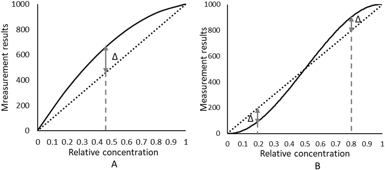
The introduced degree of non-linearity is defined as the largest difference between the quadratic or cubic regression line with the linear regression line (Δ) divided by the maximum range of measurement. Δ is located at the relative concentration(s) of (A) 0.5 for quadratic, (B) 0.2 and 0.8 for the cubic dataset.
Results
Using data that represents ‘true’ linear trend (i.e. data sets without non-linearity), the ADL false detection rate was generally lower when imprecision was low (CV=3 %) but rose considerably approaching 35 % at higher CV (10 %) (Table 2). By increasing the number of equidistant concentration points and replicate measurements, there was an improvement (reduction) in the false detection rate, with the latter having the greatest impact. There was a small deterioration in ADL performance of no more than 3 % at a high range ratio (1:1,000) when compared to the low range ratio (1:10). A measurement procedure with a high range ratio has a high ratio of maximum to minimum concentration of the analytical measurement range, e.g. an analytical measurement range of 3 mmol/L–3,000 mmol/L would have a range ratio of 1:1,000. Conversely, a measurement procedure with an analytical measurement range of 100 mmol/L–1,000 mmol/L would have a low range ratio of 1:10.
Percentage false detection rate based on average deviation from linearity (ADL) and individual deviation from linearity (IDL) methods for underlying linear simulated data.
| CV | n | Range ratio | ||||||||||||||||
|---|---|---|---|---|---|---|---|---|---|---|---|---|---|---|---|---|---|---|
| 1:10 | 1:1,000 | |||||||||||||||||
| Average deviation from linearity (ADL quadratic) | Individual deviation from linearity (IDL quadratic) | Average deviation from linearity (ADL cubic) | Individual deviation from linearity (IDL cubic) | Average deviation from linearity (ADL quadratic) | Individual deviation from linearity (IDL quadratic) | Average deviation from linearity (ADL cubic) | Individual deviation from linearity (IDL cubic) | |||||||||||
| Limit | 5 % | 10 % | 5 % | 10 % | 5 % | 10 % | 5 % | 10 % | 5 % | 10 % | 5 % | 10 % | 5 % | 10 % | 5 % | 10 % | ||
| Singlicate | 3 % | 5 | 0.2 | 0.0 | 0.9 | 0.0 | 1.3 | 0.0 | 57.2 | 22.3 | 0.3 | 0.0 | 1.3 | 0.0 | 1.3 | 0.0 | 57.1 | 22.3 |
| 6 | 0.1 | 0.0 | 1.0 | 0.0 | 0.7 | 0.0 | 58.8 | 23.1 | 0.1 | 0.0 | 1.6 | 0.0 | 0.8 | 0.0 | 59.8 | 22.9 | ||
| 10 % | 5 | 35.0 | 6.3 | 43.4 | 11.8 | 58.1 | 16.0 | 94.1 | 79.7 | 37.2 | 7.8 | 45.3 | 13.8 | 57.4 | 15.8 | 94 | 79.2 | |
| 6 | 30.5 | 4.2 | 44.2 | 12.4 | 52.6 | 12.2 | 94.6 | 80.8 | 33.4 | 5.4 | 47.0 | 15.1 | 52.8 | 12.4 | 94.6 | 81.1 | ||
| Duplicate | 3 % | 5 | 0.0 | 0.0 | 50.4 | 17.7 | 0.0 | 0.0 | 39.8 | 8.8 | 0.0 | 0.0 | 99.5 | 98.9 | 0.1 | 0.0 | 99.3 | 98.5 |
| 6 | 0.0 | 0.0 | 50.4 | 18.4 | 0.0 | 0.0 | 40.6 | 8.7 | 0.0 | 0.0 | 99.4 | 98.9 | 0.0 | 0.0 | 99.3 | 98.5 | ||
| 10 % | 5 | 18.1 | 0.8 | 83.6 | 67.7 | 36.1 | 3.9 | 88.8 | 65.6 | 21.2 | 1.5 | 99.8 | 99.7 | 39.0 | 5.4 | 99.9 | 99.7 | |
| 6 | 14.0 | 0.3 | 84.4 | 69.9 | 30.7 | 2.4 | 89.7 | 67.5 | 17.0 | 0.8 | 99.8 | 99.7 | 34.0 | 3.6 | 99.9 | 99.7 | ||
| Triplicate | 3 % | 5 | 0.0 | 0.0 | 40.9 | 9.6 | 0.0 | 0.0 | 29.8 | 3.7 | 0.0 | 0.0 | 99.3 | 98.6 | 0.0 | 0.0 | 99.3 | 98.5 |
| 6 | 0.0 | 0.0 | 41.8 | 10.3 | 0.0 | 0.0 | 30.1 | 3.7 | 0.0 | 0.0 | 99.3 | 98.5 | 0.0 | 0.0 | 99.2 | 98.3 | ||
| 10 % | 5 | 10.2 | 0.1 | 80.2 | 61.5 | 23.2 | 1.0 | 83.6 | 55.4 | 12.7 | 0.2 | 99.8 | 99.6 | 26.0 | 1.7 | 99.8 | 99.5 | |
| 6 | 7.7 | 0.0 | 80.6 | 63.3 | 18.7 | 0.5 | 84.8 | 57.2 | 9.7 | 0.1 | 99.8 | 99.6 | 22.0 | 1.0 | 99.9 | 99.6 | ||
The false positive rate of IDL is generally much greater than ADL since an assessment is performed at each concentration level (Table 2). Similar to ADL, higher assay imprecision (10 %) is associated with a higher false positive rate. In contrast to ADL, increasing the number of samples and replicate measurements generally increased the false positive rates of IDL. Of concern is the markedly elevated IDL false positive rate at the higher range ratio, particularly in the setting of replicate measurements.
In general, the false positive rate for the residual of linear regression approaches is greater than the deviation from the ADL and IDL approaches (Tables 2 and 3). The false positive rate of the average residual approach declines with increased replicates but increases with the increased number of concentration points. By contrast, the individual residual approach had an increased false positive rate when a higher number of samples or replicate measurements was used. At the higher imprecision (CV=10 %), the false positive rates of the residual of linear regression approaches are >50 % except when a high linearity acceptance limit (10 %) is used with multiple replicate measurements.
Percentage false detection rate based on regression residual approaches for underlying linear data.
| CV | n | Range ratio | ||||||||
|---|---|---|---|---|---|---|---|---|---|---|
| 1:10 | 1:1,000 | |||||||||
| Average residual | Individual residual | Average residual | Individual residual | |||||||
| Limit | 5 % | 10 % | 5 % | 10 % | 5 % | 10 % | 5 % | 10 % | ||
| Singlicate | 3 % | 5 | 24.7 | 0.9 | 24.7 | 0.9 | 27.9 | 1.2 | 27.9 | 1.2 |
| 6 | 33.4 | 1.2 | 33.4 | 1.2 | 37.7 | 2.1 | 37.7 | 2.1 | ||
| 10 % | 5 | 90.6 | 60.7 | 90.6 | 60.7 | 91.0 | 62.4 | 91.0 | 62.4 | |
| 6 | 96.2 | 73.1 | 96.2 | 73.1 | 95.9 | 74.4 | 95.9 | 74.4 | ||
| Duplicate | 3 % | 5 | 6.9 | 0.0 | 65.1 | 6.3 | 9.2 | 0.1 | 70.0 | 9.4 |
| 6 | 10.2 | 0.0 | 74.0 | 8.4 | 13.6 | 0.1 | 78.2 | 12.5 | ||
| 10 % | 5 | 79.4 | 35.8 | 99.8 | 94.3 | 80.5 | 39.4 | 99.9 | 95.2 | |
| 6 | 88.9 | 47.3 | 100.0 | 97.4 | 89.5 | 51.3 | 100.0 | 97.7 | ||
| Triplicate | 3 % | 5 | 2.1 | 0.0 | 84.5 | 13.0 | 3.6 | 0.0 | 87.8 | 19.6 |
| 6 | 3.6 | 0.0 | 89.7 | 16.3 | 5.4 | 0.0 | 92.5 | 23.8 | ||
| 10 % | 5 | 68.7 | 22.0 | 100.0 | 99.2 | 27.9 | 1.2 | 100.0 | 99.4 | |
| 6 | 80.4 | 30.3 | 100.0 | 99.8 | 37.7 | 2.1 | 100.0 | 99.8 | ||
From the data sets that represents ‘true’ non-linear trends (i.e. data sets containing varying degrees of non-linearity), displayed in Table 4 is the power (detection capability) for underlying true non-linear quadratic and cubic simulated data for ADL and IDL when applied in quadratics or cubic detection strategies. In general, the power for detection of non-linearity is higher when the polynomial regression model matches the true underlying non-linear trend in simulated data. Subsequently, in this paper, results relating to ADL and IDL approaches are only shown in cases where the polynomial regression model and underlying data trend are matched, i.e. quadratic polynomial performance is benchmarked against underlying quadratic polynomial simulated data trends.
Percentage non-linearity detection rate based on average deviation from linearity (ADL) and individual deviation from linearity (IDL) with matched and mismatched quadratic and cubic regression models. Degree of non-linearity for underlying (quadratic or cubic) data=10 %; range ratio=1:10.
| CV | n | Underlying quadratic data | Underlying cubic data | |||||||||||||||
|---|---|---|---|---|---|---|---|---|---|---|---|---|---|---|---|---|---|---|
| Average deviation from linearity (ADL quadratic) | Individual deviation from linearity (IDL quadratic) | Average deviation from linearity (ADL cubic) | Individual deviation from linearity (IDL cubic) | Average deviation from linearity (ADL quadratic) | Individual deviation from linearity (IDL quadratic) | Average deviation from linearity (ADL cubic) | Individual deviation from linearity (IDL cubic) | |||||||||||
| Limit | 5 % | 10 % | 5 % | 10 % | 5 % | 10 % | 5 % | 10 % | 5 % | 10 % | 5 % | 10 % | 5 % | 10 % | 5 % | 10 % | ||
| Singlicate | 3 % | 5 | 90.0 | 2.5 | 96.5 | 18.3 | 93.0 | 3.7 | 100.0 | 100.0 | 0.2 | 0.0 | 0.9 | 0.0 | 100.0 | 61.4 | 100.0 | 100.0 |
| 6 | 87.3 | 0.8 | 98.0 | 26.8 | 90.5 | 1.2 | 100.0 | 100.0 | 0.1 | 0.0 | 1.2 | 0.0 | 100.0 | 59.7 | 100.0 | 100.0 | ||
| 10 % | 5 | 66.5 | 28.4 | 72.6 | 39.8 | 82.1 | 37.4 | 98.6 | 94.6 | 35 | 6.4 | 43.5 | 11.8 | 95.6 | 62.6 | 99.8 | 99.2 | |
| 6 | 63.7 | 23.3 | 73.8 | 42.4 | 80.3 | 32.1 | 98.9 | 96.0 | 30.5 | 4.4 | 44.1 | 13.0 | 95.7 | 60.5 | 99.9 | 99.7 | ||
| Duplicate | 3 % | 5 | 96.5 | 0.3 | 100.0 | 100.0 | 97.6 | 0.5 | 100.0 | 100.0 | 0.0 | 0.0 | 51.3 | 18.6 | 100.0 | 64.6 | 100.0 | 100.0 |
| 6 | 94.7 | 0.0 | 100.0 | 100.0 | 96.3 | 0.1 | 100.0 | 100.0 | 0.0 | 0.0 | 50.8 | 19.2 | 100.0 | 61.1 | 100.0 | 100.0 | ||
| 10 % | 5 | 70.3 | 20.4 | 97.6 | 94.8 | 82.1 | 25.0 | 99.1 | 97.2 | 18.8 | 0.8 | 84.4 | 68.9 | 98.2 | 60.0 | 100.0 | 99.9 | |
| 6 | 68.9 | 15.3 | 98.0 | 95.7 | 79.8 | 19.7 | 99.5 | 98.1 | 14.7 | 0.4 | 84.9 | 70.0 | 98.3 | 57.8 | 100.0 | 100.0 | ||
| Triplicate | 3 % | 5 | 98.6 | 0.0 | 100.0 | 100.0 | 99.2 | 0.1 | 100.0 | 100.0 | 0.0 | 0.0 | 41.2 | 10.2 | 100.0 | 66.1 | 100.0 | 100.0 |
| 6 | 97.6 | 0.0 | 100.0 | 100.0 | 98.4 | 0.0 | 100.0 | 100.0 | 0.0 | 0.0 | 42.5 | 11.3 | 100.0 | 63.7 | 100.0 | 100.0 | ||
| 10 % | 5 | 75.0 | 15.6 | 98.8 | 97.2 | 83.7 | 19.0 | 99.7 | 98.9 | 10.7 | 0.1 | 80.8 | 63.0 | 99.0 | 58.8 | 100.0 | 100.0 | |
| 6 | 72.7 | 10.7 | 99.1 | 98.0 | 80.6 | 13.9 | 99.8 | 99.3 | 7.7 | 0.1 | 81.3 | 63.0 | 99.3 | 57.5 | 100.0 | 100.0 | ||
In contrast to IDL, the ADL approach generally had lower power for detection of non-linearity particularly when the non-linearity acceptance limit is wide (10 %), relative to the degree of introduced non-linearity (5 %) (Table 5). When the non-linearity acceptance limit (5 %) is set the same as the degree of non-linearity (5 %), the power for detection of non-linearity of the ADL method still remain sub-optimal (<80 %). Quadratic data was generally associated with lower non-linearity detection rates. A high range ratio (1:1,000 vs. 1:10) improves non-linearity detection, as does higher imprecision (10 vs. 3 %). Increasing the number of samples and replicates decreases the non-linearity detection rate with the ADL approach. The opposite is observed with IDL where a higher number of sample and replicate measurements is associated with increased power for detection of non-linearity. When a non-linearity of 10 % is introduced, it is generally well detected by a narrower non-linearity acceptance limit (5 %) (Table 6) and has a lower power for detection of non-linearity when the ADL approach is applied to data with underlying quadratic trends.
Percentage non-linearity detection rate based on average deviation from linearity (ADL) and individual deviation from linearity (IDL) with quadratic and cubic regression. Degree of non-linearity for underlying data=5 %; quadratic data is fitted with matched quadratic regression models while cubic data is fitted with cubic regression models.
| CV | n | Range ratio | ||||||||||||||||
|---|---|---|---|---|---|---|---|---|---|---|---|---|---|---|---|---|---|---|
| 1:10 | 1:1,000 | |||||||||||||||||
| Average deviation from linearity (ADL quadratic) | Individual deviation from linearity (IDL quadratic) | Average deviation from linearity (ADL cubic) | Individual deviation from linearity (IDL cubic) | Average deviation from linearity (ADL quadratic) | Individual deviation from linearity (IDL quadratic) | Average deviation from linearity (ADL cubic) | Individual deviation from linearity (IDL cubic) | |||||||||||
| Limit | 5 % | 10 % | 5 % | 10 % | 5 % | 10 % | 5 % | 10 % | 5 % | 10 % | 5 % | 10 % | 5 % | 10 % | 5 % | 10 % | ||
| Singlicate | 3 % | 5 | 19.2 | 0.0 | 36.5 | 0.1 | 58.7 | 0.3 | 99.9 | 97.4 | 27.4 | 0.0 | 44.9 | 0.6 | 70.9 | 0.9 | 100.0 | 100.0 |
| 6 | 14.2 | 0.0 | 42.5 | 0.2 | 57.5 | 0.2 | 100.0 | 99.5 | 21.4 | 0.0 | 50.9 | 0.7 | 70.2 | 0.6 | 100.0 | 100.0 | ||
| 10 % | 5 | 44.3 | 11.9 | 52.3 | 19.3 | 74.6 | 28.2 | 97.5 | 90.4 | 47.8 | 14.6 | 55.4 | 22.5 | 78.8 | 32.4 | 100.0 | 99.9 | |
| 6 | 40.9 | 9.0 | 53.6 | 21.1 | 72.7 | 24.2 | 98.2 | 92.9 | 44.2 | 11.7 | 57.0 | 24.7 | 77.3 | 28.6 | 100.0 | 100.0 | ||
| Duplicate | 3 % | 5 | 11.1 | 0.0 | 99.5 | 97.4 | 58.8 | 0.0 | 100.0 | 99.4 | 19.6 | 0.0 | 100.0 | 100.0 | 75.0 | 0.0 | 100.0 | 100.0 |
| 6 | 6.4 | 0.0 | 99.8 | 98.6 | 57.3 | 0.0 | 100.0 | 100.0 | 12.9 | 0.0 | 100.0 | 100.0 | 75.0 | 0.0 | 100.0 | 100.0 | ||
| 10 % | 5 | 36.8 | 4.5 | 90.1 | 80.1 | 68.0 | 14.4 | 97.8 | 90.4 | 40.7 | 6.5 | 99.9 | 99.8 | 73.3 | 18.5 | 100.0 | 99.9 | |
| 6 | 33.1 | 2.7 | 91.2 | 82.2 | 65.6 | 11.6 | 98.7 | 93.8 | 37.6 | 4.4 | 99.9 | 99.8 | 71.4 | 15.4 | 100.0 | 100.0 | ||
| Triplicate | 3 % | 5 | 6.9 | 0.0 | 99.9 | 99.3 | 59.2 | 0.0 | 100.0 | 99.9 | 14.7 | 0.0 | 100.0 | 100.0 | 78.6 | 0.0 | 100.0 | 100.0 |
| 6 | 3.2 | 0.0 | 100.0 | 99.6 | 57.7 | 0.0 | 100.0 | 100.0 | 8.6 | 0.0 | 100.0 | 100.0 | 78.2 | 0.0 | 100.0 | 100.0 | ||
| 10 % | 5 | 33.0 | 1.7 | 90.9 | 81.5 | 64.2 | 8.7 | 98.4 | 91.0 | 37.9 | 3.2 | 99.9 | 99.8 | 71.6 | 12.4 | 100.0 | 100.0 | |
| 6 | 28.8 | 0.9 | 91.4 | 82.9 | 62.0 | 6.3 | 99.1 | 95.0 | 34.0 | 1.9 | 99.9 | 99.8 | 69.6 | 10.2 | 100.0 | 100.0 | ||
Non-linearity detection rate (in percentage) based average deviation from linearity (ADL) and individual deviation from linearity (IDL) with quadratic and cubic regression. Degree of non-linearity for underlying data=10 %; quadratic data is fitted with quadratic regression models, while cubic data is fitted with cubic regression models.
| CV | n | Range ratio | ||||||||||||||||
|---|---|---|---|---|---|---|---|---|---|---|---|---|---|---|---|---|---|---|
| 1:10 | 1:1,000 | |||||||||||||||||
| Average deviation from linearity (ADL quadratic) | Individual deviation from linearity (IDL quadratic) | Average deviation from linearity (ADL cubic) | Individual deviation from linearity (IDL cubic) | Average deviation from linearity (ADL quadratic) | Individual deviation from linearity (IDL quadratic) | Average deviation from linearity (ADL cubic) | Individual deviation from linearity (IDL cubic) | |||||||||||
| Limit | 5 % | 10 % | 5 % | 10 % | 5 % | 10 % | 5 % | 10 % | 5 % | 10 % | 5 % | 10 % | 5 % | 10 % | 5 % | 10 % | ||
| Singlicate | 3 % | 5 | 90.0 | 2.5 | 96.5 | 18.3 | 100.0 | 61.4 | 100.0 | 100.0 | 94.3 | 7.7 | 98.1 | 32.5 | 100.0 | 82.2 | 100.0 | 100.0 |
| 6 | 87.3 | 0.8 | 98.0 | 26.8 | 100.0 | 59.7 | 100.0 | 100.0 | 93.1 | 3.2 | 98.9 | 42.7 | 100.0 | 81.7 | 100.0 | 100.0 | ||
| 10 % | 5 | 66.5 | 28.4 | 72.6 | 39.8 | 95.6 | 62.6 | 99.8 | 99.2 | 68.8 | 32.9 | 74.9 | 44.0 | 97.5 | 70.3 | 100.0 | 100.0 | |
| 6 | 63.7 | 23.3 | 73.8 | 42.4 | 95.7 | 60.5 | 99.9 | 99.7 | 67.3 | 28.9 | 76.8 | 47.5 | 97.8 | 69.3 | 100.0 | 100.0 | ||
| Duplicate | 3 % | 5 | 96.5 | 0.3 | 100.0 | 100.0 | 100.0 | 64.6 | 100.0 | 100.0 | 98.7 | 2.0 | 100.0 | 100.0 | 100.0 | 89.4 | 100.0 | 100.0 |
| 6 | 94.7 | 0.0 | 100.0 | 100.0 | 100.0 | 61.1 | 100.0 | 100.0 | 98.2 | 0.5 | 100.0 | 100.0 | 100.0 | 89.2 | 100.0 | 100.0 | ||
| 10 % | 5 | 70.3 | 20.4 | 97.6 | 94.8 | 98.2 | 60.0 | 100.0 | 99.9 | 74.5 | 26.5 | 100.0 | 100.0 | 99.1 | 70.8 | 100.0 | 100.0 | |
| 6 | 68.9 | 15.3 | 98.0 | 95.7 | 98.3 | 57.8 | 100.0 | 100.0 | 73.3 | 21.5 | 100.0 | 100.0 | 99.2 | 68.9 | 100.0 | 100.0 | ||
| Triplicate | 3 % | 5 | 98.6 | 0.0 | 100.0 | 100.0 | 100.0 | 66.1 | 100.0 | 100.0 | 98.6 | 0.0 | 100.0 | 100.0 | 100.0 | 66.5 | 100.0 | 100.0 |
| 6 | 97.6 | 0.0 | 100.0 | 100.0 | 100.0 | 63.7 | 100.0 | 100.0 | 97.7 | 0.0 | 100.0 | 100.0 | 100.0 | 63.7 | 100.0 | 100.0 | ||
| 10 % | 5 | 75.0 | 15.6 | 98.8 | 97.2 | 99.0 | 58.8 | 100.0 | 100.0 | 74.8 | 15.9 | 98.7 | 97.1 | 99.1 | 58.6 | 100.0 | 100.0 | |
| 6 | 72.7 | 10.7 | 99.1 | 98.0 | 99.3 | 57.5 | 100.0 | 100.0 | 72.2 | 10.9 | 99.1 | 97.9 | 99.3 | 57.5 | 100.0 | 100.0 | ||
The power for detection of non-linearity for the residual of the linear regression approaches are generally higher than the deviation from linearity approaches (Tables 6 and 7), with the individual residual approach having higher power for detection of non-linearity than the average residual approach. However, these approaches are generally associated with high false detection rate. A smaller imprecision (3 %), a larger degree of non-linearity (relative to the acceptance limit), a higher number of samples, and replicate measurements, combined with data that has an underlying cubic trend, are associated with higher power for detection of non-linearity and low false positive rate.
Non-linearity detection rate (in percentage) based on residual of linear regression for underlying quadratic and cubic data.
| Degree of non-linearity | CV | n | Underlying quadratic trend | Underlying cubic trend | |||||||||||||||
|---|---|---|---|---|---|---|---|---|---|---|---|---|---|---|---|---|---|---|---|
| Range ratio | Range ratio | ||||||||||||||||||
| 1:10 | 1:1,000 | 1:10 | 1:1,000 | ||||||||||||||||
| Individual residual | Average residual | Individual residual | Average residual | Individual residual | Average residual | Individual residual | Average residual | ||||||||||||
| Limit | 5 % | 10 % | 5 % | 10 % | 5 % | 10 % | 5 % | 10 % | 5 % | 10 % | 5 % | 10 % | 5 % | 10 % | 5 % | 10 % | |||
| 5 % | Singlicate | 3 % | 5 | 66.6 | 5.2 | 66.6 | 5.2 | 73.1 | 8.1 | 73.1 | 8.1 | 98.4 | 25.1 | 98.4 | 25.1 | 99.9 | 33.5 | 99.9 | 33.5 |
| 6 | 76.4 | 7.4 | 76.4 | 7.4 | 81.4 | 12.0 | 81.4 | 12.0 | 98.8 | 22.9 | 98.8 | 22.9 | 100.0 | 30.8 | 100.0 | 30.8 | |||
| 10 % | 5 | 93.5 | 66.3 | 93.5 | 66.3 | 94.0 | 68.3 | 94.0 | 68.3 | 97.0 | 73.1 | 97.0 | 73.1 | 98.1 | 75.6 | 98.1 | 75.6 | ||
| 6 | 97.5 | 77.4 | 97.5 | 77.4 | 97.4 | 78.6 | 97.4 | 78.6 | 98.9 | 81.9 | 98.9 | 81.9 | 99.5 | 83.4 | 99.5 | 83.4 | |||
| Duplicate | 3 % | 5 | 94.6 | 24.9 | 59.1 | 0.6 | 96.3 | 34.2 | 68.8 | 1.3 | 100.0 | 53.4 | 99.7 | 16.6 | 100.0 | 63.1 | 100.0 | 25.4 | |
| 6 | 96.5 | 28.1 | 68.7 | 1.3 | 98.2 | 37.8 | 77.7 | 2.6 | 100.0 | 52.7 | 99.6 | 11.6 | 100.0 | 63.9 | 100.0 | 19.9 | |||
| 10 % | 5 | 99.9 | 96.0 | 87.8 | 46.2 | 99.9 | 96.7 | 89.1 | 49.5 | 100.0 | 97.7 | 96.1 | 56.9 | 100.0 | 98.1 | 98.1 | 61.1 | ||
| 6 | 100.0 | 98.3 | 93.8 | 57.0 | 100.0 | 98.5 | 94.2 | 61.2 | 100.0 | 98.8 | 98.4 | 64.9 | 100.0 | 99.0 | 99.5 | 68.8 | |||
| Triplicate | 3 % | 5 | 99.1 | 40.9 | 68.1 | 2.3 | 99.6 | 52.5 | 76.9 | 4.5 | 100.0 | 70.8 | 99.8 | 18.4 | 100.0 | 80.1 | 100.0 | 27.6 | |
| 6 | 99.6 | 44.5 | 74.4 | 3.2 | 99.8 | 56.5 | 82.9 | 6.5 | 100.0 | 71.4 | 99.7 | 15.5 | 100.0 | 81.4 | 100.0 | 23.7 | |||
| 10 % | 5 | 100.0 | 99.5 | 95.3 | 60.6 | 100.0 | 99.6 | 95.9 | 65.0 | 100.0 | 99.8 | 98.4 | 69.6 | 100.0 | 99.8 | 99.4 | 73.8 | ||
| 6 | 100.0 | 99.9 | 97.7 | 68.4 | 100.0 | 99.9 | 97.9 | 72.8 | 100.0 | 99.9 | 99.5 | 75.5 | 100.0 | 100.0 | 99.8 | 79.0 | |||
| 10 % | Singlicate | 3 % | 5 | 99.7 | 46.0 | 99.7 | 46.0 | 99.8 | 59.4 | 99.8 | 59.4 | 100.0 | 100.0 | 100.0 | 100.0 | 100.0 | 100.0 | 100.0 | 100.0 |
| 6 | 99.9 | 53.7 | 99.9 | 53.7 | 100.0 | 67.0 | 100.0 | 67.0 | 100.0 | 100.0 | 100.0 | 100.0 | 100.0 | 100.0 | 100.0 | 100.0 | |||
| 10 % | 5 | 97.2 | 78.8 | 97.2 | 78.8 | 98.0 | 81.7 | 98.0 | 81.7 | 100.0 | 97.3 | 100.0 | 97.3 | 100.0 | 99.4 | 100.0 | 99.4 | ||
| 6 | 99.1 | 87.0 | 99.1 | 87.0 | 99.2 | 88.3 | 99.2 | 88.3 | 100.0 | 98.9 | 100.0 | 98.9 | 100.0 | 99.9 | 100.0 | 99.9 | |||
| Duplicate | 3 % | 5 | 100.0 | 81.0 | 100.0 | 34.3 | 100.0 | 89.4 | 100.0 | 53.5 | 100.0 | 100.0 | 100.0 | 100.0 | 100.0 | 100.0 | 100.0 | 100.0 | |
| 6 | 100.0 | 84.5 | 100.0 | 40.8 | 100.0 | 91.3 | 100.0 | 59.2 | 100.0 | 100.0 | 100.0 | 100.0 | 100.0 | 100.0 | 100.0 | 100.0 | |||
| 10 % | 5 | 100.0 | 98.5 | 97.0 | 69.4 | 100.0 | 98.9 | 97.9 | 73.5 | 100.0 | 100.0 | 100.0 | 98.6 | 100.0 | 100.0 | 100.0 | 100.0 | ||
| 6 | 100.0 | 99.4 | 98.8 | 78.3 | 100.0 | 99.6 | 99.1 | 81.5 | 100.0 | 100.0 | 100.0 | 99.2 | 100.0 | 100.0 | 100.0 | 100.0 | |||
| Triplicate | 3 % | 5 | 100.0 | 93.2 | 100.0 | 41.7 | 100.0 | 97.2 | 100.0 | 59.1 | 100.0 | 100.0 | 100.0 | 100.0 | 100.0 | 100.0 | 100.0 | 100.0 | |
| 6 | 100.0 | 94.7 | 100.0 | 45.0 | 100.0 | 97.9 | 100.0 | 64.9 | 100.0 | 100.0 | 100.0 | 100.0 | 100.0 | 100.0 | 100.0 | 100.0 | |||
| 10 % | 5 | 100.0 | 99.9 | 99.3 | 79.2 | 100.0 | 99.9 | 99.5 | 83.1 | 100.0 | 100.0 | 100.0 | 99.1 | 100.0 | 100.0 | 100.0 | 100.0 | ||
| 6 | 100.0 | 100.0 | 99.7 | 84.9 | 100.0 | 100.0 | 99.9 | 87.9 | 100.0 | 100.0 | 100.0 | 99.6 | 100.0 | 100.0 | 100.0 | 100.0 | |||
Discussion
Linearity is an important characteristic of a measurement procedure that requires careful assessment for its fitness for purpose [13]. This study examined four different approaches for linearity assessment (1) deviation from linearity – individual (IDL); (2) deviation from linearity – average (ADL); (3) residual – individual; and (4) residual – average. A comparison of their false detection and power for detection of non-linearity was reported. This assessment provides evidence to guide laboratory practitioners in their performances under different scenarios.
Across the four different approaches (deviation from linearity – individual and average, residual – individual and average), a major factor associated with high false detection rates is analytical imprecision. The influence of high assay imprecision can be reduced using more replicate measurements and subsequently averaging observed results. Additionally, in the deviation from linearity approaches, higher false detection rates are observed when cubic regression models are applied, in comparison to quadratic regression models.
Power for detection of non-linearity can be improved by using the polynomial regression model that matches the underlying trend of the data. Given the true underlying trend of the data is generally unknown, in addition to linear modelling both quadratic and cubic regression models should be applied concurrently to the dataset. However, this may increase the overall false detection rate, which is the sum of the false detection rate of quadratic and cubic regression approaches. In scenarios where non-linearity reside mostly in one end of the measurement range (e.g. at the higher concentration end), the quadratic regression may better detect the deviation and reject the non-linearity.
From the results of the study, deviations from linearity both average and individual, are suboptimal for detecting relatively small departures (5 %) from linearity, as these approaches are either associated with a high false detection rate and/or marginal power for detection of non-linearity. However, a high power for detection of non-linearity (>80 %) combined with a low false positive rate (<10 %) can be achieved by using the IDL approach, following the conditions/constraints, low imprecision (3 %); low range ratio (1:10); replicate measurements; small non-linearity acceptance limit and regression model matched to the underlying trend in the data (cubic in this case).
For larger departures from linearity (10 %), the ADL approach achieves >95 % power for detection of non-linearity with <1 % false detection rates when assay imprecision is small, replicate measurements are performed and when a relatively small non-linearity acceptance limit (to increase the power of detection) is used.
For the residual of regression approaches, a small degree of non-linearity (5 %) with the underlying cubic trend can be detected with >95 % probability but at the expense of high false positive rates. On the other hand, <10 % false detection rate was observed if the average residual approach is used with a low imprecision measurement procedure and replicate measurements are performed. By contrast, a large degree of non-linearity (10 %) with an underlying quadratic or cubic trend can be detected with a power for detection of non-linearity of >95 %, albeit with high false positive rates. Similarly, a false positive rate of generally <10 % was reached for measurement procedures with low imprecision and with replicate analysis.
The following suggestions are provided to laboratory practitioners when performing linearity assessment:
A high imprecision can challenge linearity investigations by producing a high false positive rate or low power of detection. Therefore, the imprecision of the measurement procedure should be considered when interpreting linearity assessment results. In the presence of high imprecision, the results of linearity assessment should be interpreted with caution.
Different linearity assessment approaches examined in this study performed well under different analytical scenarios. For optimal outcomes, a considered and tailored study design should be implemented.
Providing assay imprecision is low:
Measurement procedures with a low range ratio (1:10) and a suspected small linearity departure, may be best detected by the IDL approach when triplicate measurements are undertaken (power >95 %; false detection rate <10 %) with a relatively large allowance for non-linearity (acceptance limit) of 10 % is budgeted.
Measurement procedures with a high range ratio (1:1,000) and a suspected small linearity departure, may be best detected by the IDL approach when a triplicate measurement is performed (power >95 %; false detection rate <5 %) and a small non-linearity acceptance limit (5 %) is adopted.
For a suspected large degree of non-linearity, ADL with at least duplicate measurements combined with a relatively small non-linearity acceptance limit (5 %) will produce a power of detection of >95 % and a false positive rate of <5 %.
Averaged residual of linear regression with triplicate measurements with a non-linearity acceptance limit of 5 % produces a low false positive rate of <5 % and a high power for detection of non-linearity of >70 % across different types and degrees of non-linearity.
Conclusions
This study successfully explored four different statistical approaches (deviation from linearity – individual and average, residual – individual and average) for the assessment of linearity. From the results of the study, with the exception of specific scenarios, both ADL and IDL methods were suboptimal for the assessment of linearity compared. Detection of departures from linearity are difficult to identify in practice and enhanced methods of detection need development.
-
Research ethics: Not applicable as this study involves only computer simulations.
-
Informed consent: Not applicable as this study involves only computer simulations.
-
Author contributions: The authors have accepted responsibility for the entire content of this manuscript and approved its submission.
-
Competing interests: The authors state no conflict of interest.
-
Research funding: None declared.
-
Data availability: Not applicable.
References
1. Jhang, JS, Chang, CC, Fink, DJ, Kroll, MH. Evaluation of linearity in the clinical laboratory. Arch Pathol Lab Med 2004;128:44–8. https://doi.org/10.5858/2004-128-44-eolitc.Suche in Google Scholar PubMed
2. Hsieh, E, Liu, JP. On statistical evaluation of the linearity in assay validation. J Biopharm Stat 2008;18:677–90. https://doi.org/10.1080/10543400802071378.Suche in Google Scholar PubMed
3. Lum, G, Tholen, DW, Floering, DA. The usefulness of calibration verification and linearity surveys in predicting acceptable performance in graded proficiency tests. Arch Pathol Lab Med 1995;119:401–8.Suche in Google Scholar
4. Kroll, MH, Styer, PE, Vasquez, DA. Calibration verification performance relates to proficiency testing performance. Arch Pathol Lab Med 2004;128:544–8. https://doi.org/10.5858/2004-128-544-cvprtp.Suche in Google Scholar
5. Choudhury, SM, Shah, SL, Thornhill, NF, Choudhury, SM, Shah, SL, Thornhill, NF. Measures of nonlinearity–a review. In: Diagnosis of process nonlinearities and valve stiction: data driven approaches; 2008:69–75 pp.10.1007/978-3-540-79224-6_5Suche in Google Scholar
6. Killeen, AA, Long, T, Souers, R, Styer, P, Ventura, CB, Klee, GG. Verifying performance characteristics of quantitative analytical systems: calibration verification, linearity, and analytical measurement range. Arch Pathol Lab Med 2014;138:1173–81. https://doi.org/10.5858/arpa.2013-0051-cp.Suche in Google Scholar PubMed
7. Kroll, MH, Emancipator, K. A theoretical evaluation of linearity. Clin Chem 1993;39:405–13. https://doi.org/10.1093/clinchem/39.3.405.Suche in Google Scholar
8. Kroll, MH, Praestgaard, J, Michaliszyn, E, Styer, PE. Evaluation of the extent of nonlinearity in reportable range studies. Arch Pathol Lab Med 2000;124:1331–8. https://doi.org/10.5858/2000-124-1331-eoteon.Suche in Google Scholar
9. Analytical Methods Committee. Is my calibration linear? AMC Technical Briefs; 2005:1–2 pp.Suche in Google Scholar
10. Koh, NWX, Markus, C, Loh, TP, Lim, CY. Comparison of six regression-based lot-to-lot verification approaches. Clin Chem Lab Med 2022;60:1175–85. https://doi.org/10.1515/cclm-2022-0274.Suche in Google Scholar PubMed
11. Lim, CY, Markus, C, Greaves, R, Loh, TP. Difference- and regression-based approaches for detection of bias. Clin Biochem 2023;114:86–94. https://doi.org/10.1016/j.clinbiochem.2023.02.007.Suche in Google Scholar PubMed
12. Koh, NWX, Markus, C, Loh, TP, Lim, CY. Lot-to-lot reagent verification: effect of sample size and replicate measurement on linear regression approaches. Clin Chim Acta 2022;534:29–34. https://doi.org/10.1016/j.cca.2022.07.006.Suche in Google Scholar PubMed
13. Loh, TP, Cooke, BR, Markus, C, Zakaria, R, Tran, MTC, Ho, CS, et al.. Method evaluation in the clinical laboratory. Clin Chem Lab Med 2022;61:751–8. https://doi.org/10.1515/cclm-2022-0878.Suche in Google Scholar PubMed
© 2024 Walter de Gruyter GmbH, Berlin/Boston
Artikel in diesem Heft
- Frontmatter
- Editorial
- Six years of progress – highlights from the IFCC Emerging Technologies Division
- IFCC Papers
- Skin in the game: a review of single-cell and spatial transcriptomics in dermatological research
- Bilirubin measurements in neonates: uniform neonatal treatment can only be achieved by improved standardization
- Validation and verification framework and data integration of biosensors and in vitro diagnostic devices: a position statement of the IFCC Committee on Mobile Health and Bioengineering in Laboratory Medicine (C-MBHLM) and the IFCC Scientific Division
- Linearity assessment: deviation from linearity and residual of linear regression approaches
- HTA model for laboratory medicine technologies: overview of approaches adopted in some international agencies
- Considerations for applying emerging technologies in paediatric laboratory medicine
- A global perspective on the status of clinical metabolomics in laboratory medicine – a survey by the IFCC metabolomics working group
- The LEAP checklist for laboratory evaluation and analytical performance characteristics reporting of clinical measurement procedures
- General Clinical Chemistry and Laboratory Medicine
- Assessing post-analytical phase harmonization in European laboratories: a survey promoted by the EFLM Working Group on Harmonization
- Potential medical impact of unrecognized in vitro hypokalemia due to hemolysis: a case series
- Quantification of circulating alpha-1-antitrypsin polymers associated with different SERPINA1 genotypes
- Targeted ultra performance liquid chromatography tandem mass spectrometry procedures for the diagnosis of inborn errors of metabolism: validation through ERNDIM external quality assessment schemes
- Improving protocols for α-synuclein seed amplification assays: analysis of preanalytical and analytical variables and identification of candidate parameters for seed quantification
- Evaluation of analytical performance of AQUIOS CL flow cytometer and method comparison with bead-based flow cytometry methods
- IgG and kappa free light chain CSF/serum indices: evaluating intrathecal immunoglobulin production in HIV infection in comparison with multiple sclerosis
- Reference Values and Biological Variations
- Reference intervals of circulating secretoneurin concentrations determined in a large cohort of community dwellers: the HUNT study
- Sharing reference intervals and monitoring patients across laboratories – findings from a likely commutable external quality assurance program
- Verification of bile acid determination method and establishing reference intervals for biochemical and haematological parameters in third-trimester pregnant women
- Confounding factors of the expression of mTBI biomarkers, S100B, GFAP and UCH-L1 in an aging population
- Cancer Diagnostics
- Exploring evolutionary trajectories in ovarian cancer patients by longitudinal analysis of ctDNA
- Diabetes
- Evaluation of effects from hemoglobin variants on HbA1c measurements by different methods
- Letters to the Editor
- Are there any reasons to use three levels of quality control materials instead of two and if so, what are the arguments?
- Issues for standardization of neonatal bilirubinemia: a case of delayed phototherapy initiation
- The routine coagulation assays plasma stability – in the wake of the new European Federation of Clinical Chemistry and Laboratory Medicine (EFLM) biological variability database
- Improving HCV diagnosis following a false-negative anti-HCV result