Product Quality and Product Compatibility in Network Industries

Domenico Buccella; Luciano Fanti; Luca Gori

doi:10.1515/bejte-2023-0014

40% Rabatt

auf Fachbücher bei De Gruyter Brill *

Artikel

Product Quality and Product Compatibility in Network Industries

Domenico Buccella , Luciano Fanti und Luca Gori

Veröffentlicht/Copyright: 18. Dezember 2023

Veröffentlicht von

Veröffentlichen auch Sie bei De Gruyter Brill

Manuskript einreichen Informationen für Autor*innen Erkunden Sie dieses Fachgebiet

Aus der Zeitschrift The B.E. Journal of Theoretical Economics Band 24 Heft 1

Abstract

Using an appropriate game-theoretic approach, this article develops a non-cooperative two-stage game in a Cournot duopolistic network industry in which firms strategically choose whether to produce compatible goods in the first decision-making stage. Quality differentiation affects the sub-game perfect Nash equilibrium (SPNE): (i) the network effect acts differently between low- and high-quality firms, depending on their compatibility choice; (ii) if the network externality is positive (resp. negative), to produce compatible (resp. incompatible) goods is the unique SPNE; however, this equilibrium configuration leads the high-quality firm to be worse off; (iii) there is room for a side payment from the high- to the low-quality firm to deviate toward incompatibility (resp. compatibility) under positive (resp. negative) network externality. This payment represents a Pareto improvement on the firm side but not from a societal perspective, as consumers would be worse off. The article also pinpoints the social welfare outcomes corresponding to the SPNE.

Keywords: network externality; product compatibility; Cournot duopoly; quality differential

JEL Classification: L1; L2; D4

Corresponding author: Luca Gori, Department of Law, University of Pisa, Via Collegio Ricci, 10, I-56126 Pisa, PI, Italy, E-mail: luca.gori@unipi.it

Funding source: Università di Pisa

Award Identifier / Grant number: PRA_2020_64

Acknowledgments

The authors acknowledge the two anonymous reviewers of the journal for their valuable comments on an earlier draft of the manuscript. Luca Gori acknowledges financial support from the University of Pisa under the “PRA – Progetti di Ricerca di Ateneo” (Institutional Research Grants), Project No. PRA_2020_64 “Infectious diseases, health and development: economic and legal effects”. The usual disclaimer applies. This study was conducted when Domenico Buccella was a visiting scholar at the Department of Law of the University of Pisa.

Research funding: The authors declare that the University of Pisa funded this study.
Disclosure of potential conflict of interest: The authors declare that they have no conflict of interest.
Declarations of interest: None.

Appendix A

Analytical Details

Proof of Lemma 4. The proof follows by using the following line of reasoning: q i * K / K − q i * N K / N K > < 0 ⇔ a < > a * n : = 5 ( 1 − n ) + n 2 4 ( 1 − n ) + n 2 ≥ 1 and q j * K / K − q j * N K / N K > < 0 ⇔ a > < a * * n : = 4 ( 1 − n ) + n 2 5 ( 1 − n ) + n 2 ≤ 1 . Q.E.D.

Proof of Proposition 1

The proof follows from the sign of the profit differentials. If n > 0 then ΔΠ_A,i > 0, ΔΠ_B,i < 0, ΔΠ_C,i < 0, ΔΠ_A,j > 0, ΔΠ_B,j < 0 and ΔΠ_C,j < 0. If n < 0 then ΔΠ_A,i < 0, ΔΠ_B,i > 0, ΔΠ_C,i > 0, ΔΠ_A,j < 0, ΔΠ_B,j > 0 and ΔΠ_C,j > 0. Q.E.D.

Proof of Proposition 2

The proof follows by considering the sign of the profit differentials. If n > 0 and a ° ° ° n < a < a C , j n then ΔΠ_A,i > 0, ΔΠ_B,i < 0, ΔΠ_C,i < 0 and ΔΠ_A,j > 0, ΔΠ_B,j < 0, ΔΠ_C,j > 0; if n > 0 and a C , j n < a < a C , i n then ΔΠ_A,i > 0, ΔΠ_B,i < 0, ΔΠ_C,i < 0 and ΔΠ_A,j > 0, ΔΠ_B,j < 0, ΔΠ_C,j < 0; if n > 0 and a C , i n < a < a ° ° ° ° n then ΔΠ_A,i > 0, ΔΠ_B,i < 0, ΔΠ_C,i > 0 and ΔΠ_A,j > 0, ΔΠ_B,j < 0, ΔΠ_C,j < 0. If n < 0 and a ° n < a < a C , j n then ΔΠ_A,i < 0, ΔΠ_B,i > 0, ΔΠ_C,i > 0 and ΔΠ_A,j < 0, ΔΠ_B,j > 0, ΔΠ_C,j < 0; if n < 0 and a C , j n < a < a C , i n then ΔΠ_A,i < 0, ΔΠ_B,i > 0, ΔΠ_C,i > 0 and ΔΠ_A,j < 0, ΔΠ_B,j > 0, ΔΠ_C,j > 0; if n < 0 and a C , i n < a < a ° ° n then ΔΠ_A,i < 0, ΔΠ_B,i > 0, ΔΠ_C,i < 0 and ΔΠ_A,j < 0, ΔΠ_B,j > 0, ΔΠ_C,j > 0. Q.E.D.

Proof of Proposition 3

Let Δ S P i : = Π i * N K / N K − Π i * K / K be the side-payment differential of firm i and Δ S P j : = Π j * N K / N K − Π j * K / K be the side-payment differential of firm j. If a > 1 then firm i is the high-quality producer and firm j is the low-quality producer. If a < 1 then firm i is the low-quality producer and firm j is the high-quality producer. Let n > 0 (resp. n < 0). Then

for any a > 1 within the feasible region, the high-quality firm i can make a side-payment to the low-quality firm j if and only if ΔSP _i + ΔSP _j > 0 (resp. < 0 ) if and only if a > a max S P n > a C , i ( n ) , where

(A.1) a max S P n : = − − 2 n 4 + ( 18 + 2 3 ) n 3 − ( 60 + 11 3 ) n 2 + ( 84 + 18 3 ) n − 42 − 9 3 2 n 4 − 18 n 3 + 57 n 2 − 78 n + 39 ,
is the value of the relative quality index (as a function of the degree of the network effect) such that ΔSP _i + ΔSP _j = 0 when a > 1, and
for any a < 1 within the feasible region, the high-quality firm j can make a side-payment to the low-quality firm i if and only if ΔSP _i + ΔSP _j > 0 (resp. < 0 ) if and only if a < a min S P n < a C , j ( n ) , where
(A.2) a min S P ( n ) : = 2 n 4 + ( − 18 + 2 3 ) n 3 + ( 60 − 11 3 ) n 2 − ( 84 − 18 3 ) n + 42 − 9 3 2 n 4 − 18 n 3 + 57 n 2 − 78 n + 39 ,
is the value of the relative quality index (as a function of the degree of the network effect) such that ΔSP _i + ΔSP _j = 0 when a < 1, and a max S P n > a min S P n for any −1 < n < 0.634. If n > 0.634 then a min S P n > a ° ° ° ( n ) and a max S P n > a ° ° ° ° ( n ) . Q.E.D.

Compatibility and the Dimension of the Installed Base: when History Matters

The cumulated sold products of larger and older firms are higher than those of younger and smaller ones. This is indeed relevant especially in network industries as consumers enjoy – given the positive network effect – not only the consumption of products currently produced but also the stock accumulated in the past. In the words of Besen and Farrell (1994, p. 118): “A final characteristic of network markets is that history matters”. The main difference between standard and network markets is that while in the former only the existing consumer preferences and producer technologies matter to explain the market outcomes, in the latter “market equilibria often cannot be understood without knowing the pattern of technology adoption in earlier periods” (Besen and Farrell 1994, pp. 118–119), as consumers prefer product compatibility with the installed base.^[12]

Therefore, in addition to the direct network effects of the model analysed in the main text, there are also indirect effects that can increase the consumers’ demand. Indeed, the larger the number of consumers that are using a certain type of hardware, the more likely the provision of compatible hardware. This implies that the size of the installed base may increase the positive consumption externality. This also means that the larger and older the firm, the larger is its installed base. In other words, if the dimension of products sold in the past matters, history also matters for the choice of compatible or incompatible goods.

In this case, the network of firm i depends not only on the expected sales in the considered period, i.e. y _i and y _j but also on its installed base, which is defined as I _i > 0, and the installed base of rival, which is defined as I _j > 0 (if products are fully compatible between them). The installed base is the number of products sold to users in the past.^[13] Then, the only change with respect to the model discussed in the main text involves the inverse demand functions (2) and (3), which are respectively re-written in the following way:

(B.1) p i = a − q i − q j + n ( I i + k i I j + y i + k i y j ) ,

and

(B.2) p j = 1 − q j − q i + n ( I j + k j I i + y j + k j y i ) ,

where we will assume henceforth that product quality is homogeneous, that is a = 1. This is indeed useful to stress the similarities of the SPNE outcomes with the CDG with product quality studied so far, which in this model are driven by the size of the relative value of the installed base of the two firms. Standard calculations lead to equilibrium output and profits in the four different sub-games, similarly to the main text, which are summarised in Tables B.1 and B.2. To follow up on what was done previously, we consider full compatibility (K) versus incompatibility (NK).

Table B.1:

Quantities in each sub-game of the CDG with installed base. Second stage.

Firm i ↓ Firm j →	K	NK
K	q i * K / K ( I i , I j ) , q j * K / K ( I i , I j )	q i * K / N K ( I i , I j ) , q j * K / N K ( I i , I j )
NK	q i * N K / K ( I i , I j ) , q j * N K / K ( I i , I j )	q i * N K / N K ( I i , I j ) , q j * N K / N K ( I i , I j )

Table B.2:

The CDG with installed base (payoff matrix: profits). First stage.

Firm i ↓ Firm j →	K	NK
K	Π i * K / K ( I i , I j ) , Π j * K / K ( I i , I j )	Π i * K / N K ( I i , I j ) , Π j * K / N K ( I i , I j )
NK	Π i * N K / K ( I i , I j ) , Π j * N K / K ( I i , I j )	Π i * N K / N K ( I i , I j ) , Π j * N K / N K ( I i , I j )

The entries of Table B.1 are:

(B.3) q i * K / K ( I i , I j ) = 1 + n 2 − n I i − n ( 1 − n ) I j 3 − 2 n > 0 ,

iff I i > n 1 − n I j − 1 n ( 2 − n ) : = I i ° ( n ) for any n > 0 and I _i < I _i°(n) for any n < 0,

(B.4) q j * K / K ( I i , I j ) = 1 − n 1 − n I i + n ( 2 − n ) I j 3 − 2 n > 0 ,

iff I i < 1 + n ( 2 − n ) I j n ( 1 − n ) : = I i ° ° ( n ) for any n > 0 and I i > I i ° ° ( n ) for any n < 0,

(B.5) q i * N K / N K ( I i , I j ) = 1 − n + n 2 − n I i − n I j ( 3 − n ) ( 1 − n ) > 0 ,

iff I i > n I j + n − 1 n ( 2 − n ) : = I i ° ° ° ( n ) for any n > 0 and I i > I i ° ° ° ( n ) for any n < 0,

(B.6) q j * N K / N K ( I i , I j ) = 1 − n + n 2 − n I j − n I i ( 3 − n ) ( 1 − n ) > 0 ,

iff I i < 1 − n + n ( 2 − n ) I j n : = I i ° ° ° ° ( n ) for any n > 0 and I i > I i ° ° ° ° ( n ) for any n < 0,

(B.7) q i * K / N K ( I i , I j ) = 1 + n 2 − n I i − n ( 1 − n ) I j 3 1 − n + n 2 > 0 ,

iff I _i > I _i°(n) for any n > 0 and I _i < I _i°(n) for any n < 0,

(B.8) q j * K / N K ( I i , I j ) = 1 − n + n 2 − n I j − n I i 3 1 − n + n 2 > 0 ,

iff I i 0 and I i > I i ° ° ° ° ( n ) for any n < 0, and

(B.9) q i * N K / K ( I i , I j ) = 1 − n + n 2 − n I i − n I j 3 1 − n + n 2 > 0 ,

iff I i > I i ° ° ° ( n ) for any n > 0 and I i < I i ° ° ° ( n ) for any n < 0,

(B.10) q j * N K / K ( I i , I j ) = 1 − n 1 − n I i + n ( 2 − n ) I j 3 1 − n + n 2 > 0 ,

iff I i 0 and I i > I i ° ° ( n ) for any n < 0.

The entries of Table B.2 are:

(B.11) Π i * K / K ( I i , I j ) = 1 + n 2 − n I i − n 1 − n I j 2 ( 3 − 2 n ) 2 ,

(B.12) Π j * K / K ( I i , I j ) = 1 − n 1 − n I i + n ( 2 − n ) I j 2 ( 3 − 2 n ) 2 ,

(B.13) Π i * N K / N K ( I i , I j ) = 1 − n + n 2 − n I i − n I j 2 ( 3 − n ) 2 ( 1 − n ) 2 ,

(B.14) Π j * N K / N K ( I i , I j ) = 1 − n + n 2 − n I j − n I i 2 ( 3 − n ) 2 ( 1 − n ) 2 ,

(B.15) Π i * K / N K ( I i , I j ) = 1 + n 2 − n I i − n ( 1 − n ) I j 2 3 1 − n + n 2 2 ,

(B.16) Π j * K / N K ( I i , I j ) = 1 − n + n 2 − n I j − n I i 2 3 1 − n + n 2 2 ,

and

(B.17) Π i * N K / K ( I i , I j ) = 1 − n + n 2 − n I i − n I j 2 3 1 − n + n 2 2 ,

(B.18) Π j * N K / K ( I i , I j ) = 1 − n 1 − n I i + n ( 2 − n ) I j 2 3 1 − n + n 2 2 .

Proposition B.1 summarises the main SPNE outcomes of the CDG with installed base. The results of the proposition are also reported in Figure B.1, which represents a rigorous geometrical portrait of these outcomes. We recall that if I _i > I _j (resp. I _i < I _j) then firm i (resp. firm j) is the larger/older firm in the market.^[14] For simplicity, and without loss of generality, we assume I _j = 1. Then, we get the following result.

Figure B.1:

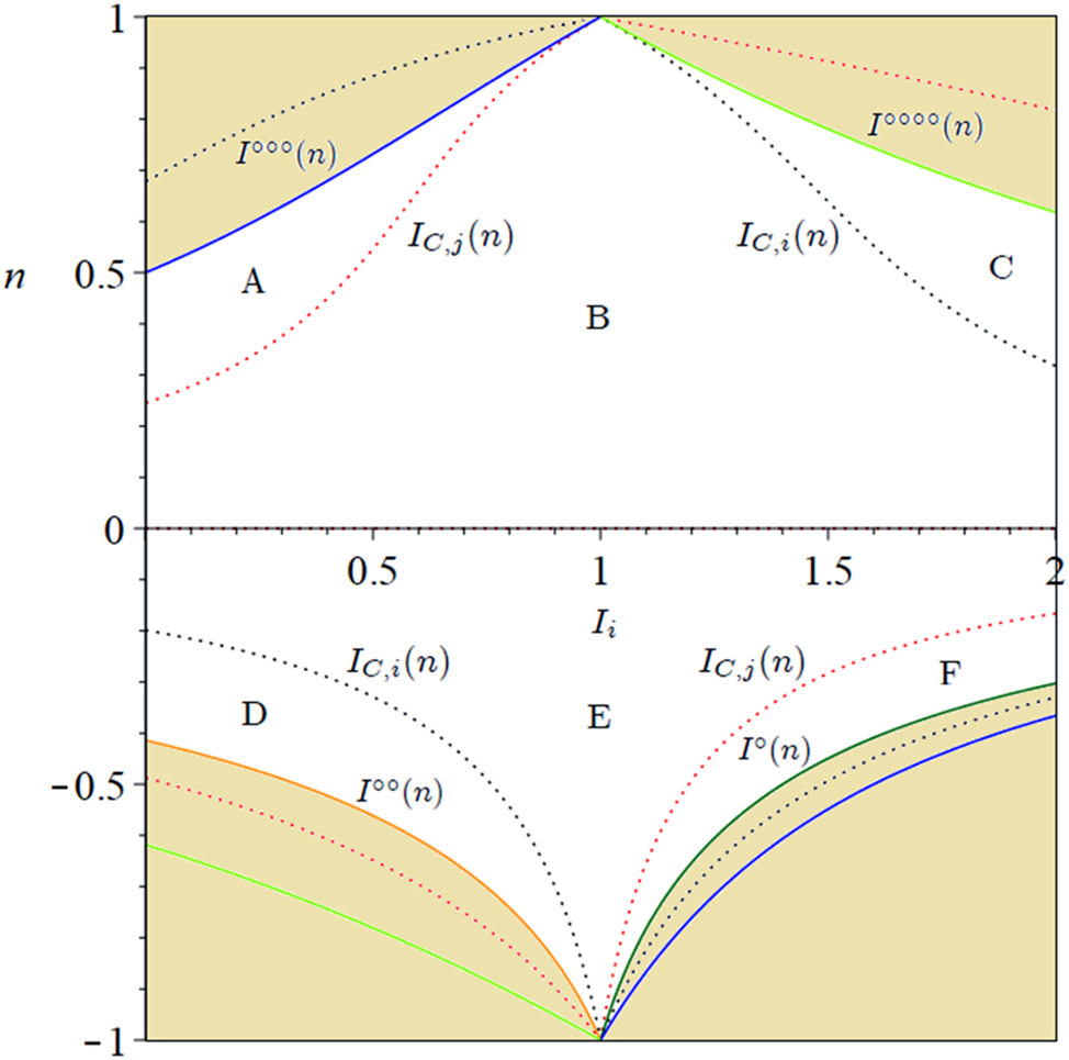
The CDG with asymmetric installed base when I _j = 1: SPNE in the space (I _i, n). The sand-coloured region is the unfeasible parameter space.

Proposition B.1

Let n > 0. Under asymmetric installed base (I _i ≠ 1), the unique SPNE of the CDG with installed base is (K, K). This equilibrium configuration is (1) such that firm j (large) is worse off if I i ° ° ° n < I i < I C , j n (firm i is the small producer in this case), (2) Pareto efficient for the players if I C , j n < I i < I C , i n , and (3) such that firm i (large) is worse off if I C , i n < I < I i ° ° ° ° n (firm j is the small producer in this case). Let n < 0. Under asymmetric installed base (I _i ≠ 1), the unique SPNE of the CDG is (NK, NK). This equilibrium configuration is (4) such that firm i (small) is worse off if I i ° ° n < I < I C , i n (firm j is the large producer in this case), (5) Pareto efficient for the players if I C , i n < I < I C , j n , and (6) such that firm j (small) is worse off if I C , j n < I < I i ° n (firm i is the large producer in this case).

Proof

The proof follows by considering the sign of the profit differentials. If n > 0 and I i ° ° ° n 0, ΔΠ_B,i(I _i, I _j) < 0, ΔΠ_C,i(I _i, I _j) < 0 and ΔΠ_A,j(I _i, I _j) > 0, ΔΠ_B,j(I _i, I _j) < 0, ΔΠ_C,j(I _i, I _j) > 0; if n > 0 and I C , j n 0, ΔΠ_B,i(I _i, I _j) < 0, ΔΠ_C,i(I _i, I _j) < 0 and ΔΠ_A,j(I _i, I _j) > 0, ΔΠ_B,j(I _i, I _j) < 0, ΔΠ_C,j(I _i, I _j) < 0; if n > 0 and I C , i n 0, ΔΠ_B,i(I _i, I _j) < 0, ΔΠ_C,i(I _i, I _j) > 0 and ΔΠ_A,j(I _i, I _j) > 0, ΔΠ_B,j(I _i, I _j) < 0, ΔΠ_C,j(I _i, I _j) < 0. If n < 0 and I i ° ° n 0, ΔΠ_C,i(I _i, I _j) < 0 and ΔΠ_A,j(I _i, I _j) < 0, ΔΠ_B,j(I _i, I _j) > 0, ΔΠ_C,j(I _i, I _j) > 0; if n < 0 and I C , i n 0, ΔΠ_C,i(I _i, I _j) > 0 and ΔΠ_A,j(I _i, I _j) < 0, ΔΠ_B,j(I _i, I _j) > 0, ΔΠ_C,j(I _i, I _j) > 0; if n < 0 and I C , j n 0, ΔΠ_C,i(I _i, I _j) > 0 and ΔΠ_A,j(I _i, I _j) < 0, ΔΠ_B,j(I _i, I _j) > 0, ΔΠ_C,j(I _i, I _j) < 0. Q.E.D.

The proposition reveals that when the network externality is positive, the unique SPNE of the CDG with asymmetric installed base is (K, K). This equilibrium configuration can be such that the large firm is worse off. This firm is indeed entrapped in a “bad” equilibrium when the relative size of the installed base is sufficiently small ( I i I C , i n ). In the former case, firm j is entrapped in a “bad” equilibrium. In the latter case, firm i is entrapped in a “bad” equilibrium, where I _C,i(n) and I _C,j(n) are the values of the relative installed base such that ΔΠ_C,i(I _i, I _j) = 0 and ΔΠ_C,j(I _i, I _j) = 0, respectively, which are defined as follows:

(B.19) I C , i n : = 1 − n + n I j 5 1 − n + n 2 n 4 1 − n + n 2 ,

and

(B.20) I C , j n = n − 1 + n I j [ 4 1 − n + n 2 ] n [ 5 1 − n + n 2 ] .

Corollary B.1

From the expressions in (B.19) and (B.20), the larger the positive network effect, the more likely the entrapment in the “bad” equilibrium for the large firm. If the network effect is sufficiently high, it is enough to have a small differential in the installed bases of the two firms for the compatibility strategy to be profit-reducing for the large firm.

Then, the large/old firm is entrapped in a “bad” equilibrium if it is sufficiently big/old. Therefore, the production of compatible products when the installed base is high benefits the smaller rival. Unfortunately, the SPNE is (K, K), which is the rational outcome obtained in the market.

Area A: (K, K) is the unique SPNE, representing a “good” equilibrium for firm i (small) and a “bad” equilibrium for firm j (large).
Area B: (K, K) is the unique SPNE, which is Pareto efficient for the players firms (the CDG with installed base is a deadlock).
Area C: (K, K) is the unique SPNE, representing a “bad” equilibrium for firm i (large) and a “good” equilibrium for firm j (small).
Area D: (NK, NK) is the unique SPNE, representing a “bad” equilibrium for firm i (small) and a “good” equilibrium for firm j (large).
Area E: (NK, NK) is the unique SPNE, which is Pareto efficient for the players (the CDG with installed base is a deadlock).
Area F: (NK, NK) is the unique SPNE, representing a “good” equilibrium for firm i (large) and a “bad” equilibrium for firm j (small).

The CDG with Asymmetric Marginal Costs

This appendix continues the study of the extensions of the model presented in the main text and considers the CDG with heterogeneous (or asymmetric) marginal costs between firm i and firm j with homogeneous (instead of heterogeneous) product quality (a = 1). Thus, the only difference from the main model, in which the marginal cost was homogeneous and normalised to zero, concerns the technological efficiency. Specifically, we assume that firm i is the most efficient incurring a marginal cost of production of c _i = 0, and firm j is the least efficient incurring a positive marginal cost of production of c _j > 0. The analysis proceeds in the same way as that considered presented in the main text, so we do not present the analytical details here, but rather directly write down the payoff matrix (Table C.1), from which profit differentials can easily be calculated, and the feasibility conditions, which are given by c j < c ° n : = 1 2 − n and c j < c ° ° n : = 1 − n 2 − n . The former (resp. latter) guarantees that the production of the least efficient firm in the sub-game K/K (resp. NK/NK) is positive. When these inequalities are fulfilled, a positive production in each sub-game is guaranteed.

Table C.1:

The CDG with asymmetric marginal costs (payoff matrix: profits). First stage.

Firm i ↓ Firm j →	K	NK
K	Π i * K / K ( c i , c j ) , Π j * K / K ( c i , c j )	Π i * K / N K ( c i , c j ) , Π j * K / N K ( c i , c j )
NK	Π i * N K / K ( c i , c j ) , Π j * N K / K ( c i , c j )	Π i * N K / N K ( c i , c j ) , Π j * N K / N K ( c i , c j )

The entries of Table C.1 are:

(C.1) Π i * K / K ( c i , c j ) = [ 1 + c ( 1 − n ) ] 2 ( 3 − 2 n ) 2 ,

(C.2) Π j * K / K ( c i , c j ) = [ 1 − c ( 2 − n ) ] 2 ( 3 − 2 n ) 2 ,

(C.3) Π i * N K / N K ( c i , c j ) = ( 1 − n + c ) 2 ( 3 − n ) 2 ( 1 − n ) 2 ,

(C.4) Π j * N K / N K ( c i , c j ) = [ 1 − n − c ( 2 − n ) ] 2 ( 3 − n ) 2 ( 1 − n ) 2 ,

(C.5) Π i * K / N K ( c i , c j ) = [ 1 + c ( 1 − n ) ] 2 [ 3 1 − n + n 2 ] 2 ,

(C.6) Π j * K / N K ( c i , c j ) = [ 1 − n − c ( 2 − n ) ] 2 [ 3 1 − n + n 2 ] 2 ,

and

(C.7) Π i * N K / K ( c i , c j ) = ( 1 + c − n ) 2 [ 3 1 − n + n 2 ] 2 ,

(C.8) Π j * N K / K ( c i , c j ) = [ 1 − c ( 2 − n ) ] 2 [ 3 1 − n + n 2 ] 2 .

Proposition C.1 summarises the main SPNE outcomes of the CDG with asymmetric marginal costs. The results of the proposition are also reported in Figure C.1, which represents a rigorous geometrical portrait of these results.

Figure C.1:

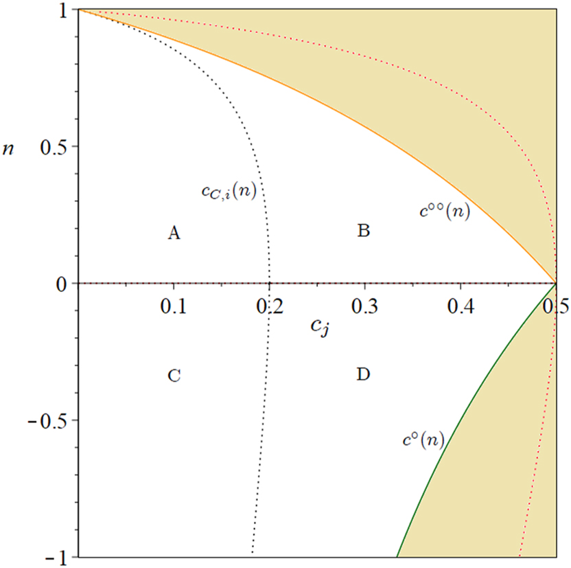
The CDG with asymmetric marginal costs when c _i = 0 and c _j > 0: SPNE in the space (c _j, n). The sand-coloured region is the unfeasible parameter space.

Proposition C.1

Let n > 0. Under asymmetric marginal costs (c _i = 0 and c _j > 0), the unique SPNE of the CDG with asymmetric marginal costs is (K, K). This equilibrium configuration is (1) Pareto efficient for firm i (the most efficient producer) and firm j (the least efficient producer) if 0 < c i < c C , i n , (2) such that firm i (the most efficient producer) is worse off if c C , i n < c i < c ° ° n (firm j is the least efficient producer in this case). Let n < 0. Under asymmetric marginal costs (c _i = 0 and c _j > 0), the unique SPNE of the CDG with asymmetric marginal costs is (NK, NK). This equilibrium configuration is (3) Pareto efficient for firm i (the most efficient producer) and firm j (the least efficient producer) if 0 < c i < c C , i n , (2) such that firm i (the most efficient producer) is worse off if c C , i n < c i < c ° n (firm j is the least efficient producer in this case), where

(C.9) c C , i n : = 1 − n 5 1 − n + n 2 ,

is the threshold value of the marginal cost such that ΔΠ_C,i(c _i, c _j) = 0.

Proof

The proof follows by considering the sign of the profit differentials. If n > 0 and 0 < c i < c C , i n then ΔΠ_A,i(c _i, c _j) > 0, ΔΠ_B,i(c _i, c _j) < 0, ΔΠ_C,i(c _i, c _j) < 0 and ΔΠ_A,j(c _i, c _j) > 0, ΔΠ_B,j(c _i, c _j) < 0, ΔΠ_C,j(c _i, c _j) < 0; if n > 0 and c C , i n < c i < c ° ° n then ΔΠ_A,i(c _i, c _j) > 0, ΔΠ_B,i(c _i, c _j) < 0, ΔΠ_C,i(c _i, c _j) > 0 and ΔΠ_A,j(c _i, c _j) > 0, ΔΠ_B,j(c _i, c _j) < 0, ΔΠ_C,j(c _i, c _j) < 0. If n < 0 and 0 < c i < c C , i n then ΔΠ_A,i(c _i, c _j) < 0, ΔΠ_B,i(c _i, c _j) > 0, ΔΠ_C,i(c _i, c _j) > 0 and ΔΠ_A,j(c _i, c _j) < 0, ΔΠ_B,j(c _i, c _j) > 0, ΔΠ_C,j(c _i, c _j) > 0; if n < 0 and c C , i n < c i < c ° n then ΔΠ_A,i(c _i, c _j) < 0, ΔΠ_B,i(c _i, c _j) > 0, ΔΠ_C,i(c _i, c _j) < 0 and ΔΠ_A,j(c _i, c _j) < 0, ΔΠ_B,j(c _i, c _j) > 0, ΔΠ_C,j(c _i, c _j) > 0. Q.E.D.

Area A: (K, K) is the unique SPNE, which is Pareto efficient for firm i (the most efficient) and firm j (the least efficient). The CDG with asymmetric marginal costs is a deadlock.
Area B: (K, K) is the unique SPNE, representing a “bad” equilibrium for firm i (the most efficient) and a “good” equilibrium for firm j (the least efficient).
Area C: (NK, NK) is the unique SPNE, which is Pareto efficient for firm i (the most efficient) and firm j (the least efficient). The CDG with asymmetric marginal costs is a deadlock.
Area D: (NK, NK) is the unique SPNE, representing a “bad” equilibrium for firm i (the most efficient) and a “good” equilibrium for firm j (the least efficient).

Then, the most efficient firm can be entrapped in a “bad” equilibrium if the marginal cost of the least efficient firm is sufficiently high. Therefore, the production of compatible (resp. incompatible) products when the marginal cost is high benefits the least efficient rival when the network externality is positive (resp. negative). Unfortunately, the SPNE is (K, K) (resp. (NK, NK)) which is the rational outcome obtained in the market. By considering together both the quality differential and cost differential, the outcomes of CDG are qualitatively the same, unless the appearance of a region in which the Nash equilibrium in pure strategy does not exists. For economy of space, we do not report this analysis here, but it is available on request.

Appendix D

The CDG with Output Commitment

This appendix follows the main analysis of Katz and Shapiro (1985), in which firm i commits itself to an announced output level and firm j does not commit itself to an announced output (asymmetric output commitment) and then evaluates the firm’s incentives to produce compatible and incompatible goods in the first stage. In doing so, we consider homogeneous quality (a = 1) and no marginal cost (c = 0). We briefly outline here the main difference to the model presented in the main text, i.e. the demands for firm i and firm j. The (normalised) inverse demand of firm i (commitment) when the rival does not commit is:

(D.1) p i = 1 − q i − q j + n ( q i + k i y j ) ,

and the (normalised) inverse demand of firm j (no commitment) when the rival commits is:

(D.2) p j = 1 − q j − q i + n ( y j + k j q i ) ,

where y _i ( i , j = 1,2 , i ≠ j) denotes the consumers’ expectations about the equilibrium output produced by firm i. We recall that (1) when both firms produce compatible goods k _i = k _j = 1 (K/K), (2) when both firms produce incompatible goods k _i = k _j = 0 (NK/NK), and (3) when only one of the two firms produces compatible goods k _i = 1 and k _j = 0 (K/NK) or vice versa (NK/K). As usual, the section does not report the analytical details, which are available on request, and directly presents the output matrix in the second stage (Table D.1) and the payoff matrix in the first decision-making stage (Table D.2) of the CDG when firm i commits itself and firm j does not commit itself to an announced output level as well as the feasibility condition, which is simply given by n < 1/2. When this inequality is fulfilled, the output produced by firms in all sub-games is positive.

Table D.1:

The CDG with output commitment (output matrix). Second stage.

Firm i ↓ Firm j →	K	NK
K	1 3 − n ( 1 − n ) , 1 3 − n	1 3 − 2 n ( 1 − n ) , 1 − 2 n ( 3 − 2 n ) ( 1 − n )
NK	1 3 − 2 n , 1 3 − 2 n	1 − n 3 1 − n 2 − n 2 , 1 − 2 n 3 1 − n 2 − n 2

Table D.2:

The CDG with output commitment (payoff matrix: profits). Second stage.

Firm i ↓ Firm j →	K	NK
K	1 3 − n 2 ( 1 − n ) , 1 3 − n 2	1 3 − 2 n 2 ( 1 − n ) , ( 1 − 2 n ) 2 ( 3 − 2 n ) 2 ( 1 − n ) 2
NK	1 − n ( 3 − 2 n ) 2 , 1 ( 3 − 2 n ) 2	( 1 − n ) 3 [ 3 1 − n 2 − n 2 ] 2 , ( 1 − 2 n ) 2 [ 3 1 − n 2 − n 2 ] 2

Proposition D.1 summarises the main SPNE outcomes of the CDG with asymmetric output commitment.

Proposition D.1

Let n > 0. Under asymmetric output commitment, the unique SPNE of the CDG with output commitment is (K, K). This equilibrium configuration is (1) Pareto efficient for firm i (that commits itself to an announced output level) and firm j (that does not commit itself to an announced output level) if 0 < n < 3 2 − 1 2 5 ≅ 0.381 , (2) such that firm i (that commits itself to an announced output level) is worse off if 0.381 < n < 0.5 (firm j is the producer that does not commit itself to an announced output level). Let n < 0. Under asymmetric output commitment, the unique SPNE of the CDG with output commitment is (NK, NK), which is (3) Pareto efficient for firm i (that commits itself to an announced output level) and firm j (that does not commit itself to an announced output level) if −1 < n < 0.

Proof

The proof follows by considering the sign of the profit differentials. If n > 0 and 0 < c _i < 0.381 then ΔΠ_A,i(n) > 0, ΔΠ_B,i(n) < 0, ΔΠ_C,i(n) < 0 and ΔΠ_A,j(n) > 0, ΔΠ_B,j(n) < 0, ΔΠ_C,j(n) < 0; if n > 0 and 0.381 < c _i < 0.5 then ΔΠ_A,i(n) > 0, ΔΠ_B,i(n) < 0, ΔΠ_C,i(n) > 0 and ΔΠ_A,j(n) > 0, ΔΠ_B,j(n) < 0, ΔΠ_C,j(n) < 0. If n < 0 then ΔΠ_A,i(n) < 0, ΔΠ_B,i(n) > 0, ΔΠ_C,i(n) > 0 and ΔΠ_A,j(n) < 0, ΔΠ_B,j(n) > 0, ΔΠ_C,j(n) > 0. Q.E.D.

The proposition reveals that, for a high positive network size, the firm that announces production and commits itself to it would find it more profitable to produce incompatible goods. This is because the commitment binds the firm to increase production, and this eventually reduces profits. Unfortunately for this firm, the SPNE that emerges in the market is to produce compatible goods and then the committing firm is worse off and entrapped in a “bad” equilibrium.

References

Amir, R., P. Erickson, and J. Jin. 2017. “On the Microeconomic Foundations of Linear Demand for Differentiated Products.” Journal of Economic Theory 169: 641–65. https://doi.org/10.1016/j.jet.2017.03.005.Suche in Google Scholar

Amir, R., I. Evstigneev, and A. Gama. 2021. “Oligopoly with Network Effects: Firm-specific versus Single Network.” Economic Theory 71: 1203–30. https://doi.org/10.1007/s00199-019-01229-0.Suche in Google Scholar

Besen, S.M., and J. Farrell. 1994. “Choosing How to Compete: Strategies and Tactics in Standardization.” The Journal of Economic Perspectives 8: 117–31. https://doi.org/10.1257/jep.8.2.117.Suche in Google Scholar

Besen, S.M. 1992. “AM versus FM: The Battle of the Bands.” Industrial and Corporate Change 1: 375–96. https://doi.org/10.1093/icc/1.2.375.Suche in Google Scholar

Bhattacharjee, T., and R. Pal. 2013. “Price vs. Quantity in a Duopoly with Strategic Delegation: The Role of Network Externalities.” Review of Network Economics 12: 343–53. https://doi.org/10.1515/rne-2013-0114.Suche in Google Scholar

Bhattacharjee, T., and R. Pal. 2014. “Network Externalities and Strategic Managerial Delegation in Cournot Duopoly: Is There a Prisoners' Dilemma?” Review of Network Economics 12: 343–53.10.1515/rne-2013-0114Suche in Google Scholar

Binmore, K.G. 2007. Game Theory: A Very Short Introduction. New York: Oxford University Press.10.1093/actrade/9780199218462.001.0001Suche in Google Scholar

Buccella, D., L. Fanti, and L. Gori. 2023a. “Network Externalities, Product Compatibility and Process Innovation.” Economics of Innovation and New Technology 32: 1156–89.10.1080/10438599.2022.2095513Suche in Google Scholar

Buccella, D., L. Fanti, and L. Gori. 2023b. “Strategic Product Compatibility in Network Industries.” Journal of Economics 140: 141–68.10.1007/s00712-023-00834-xSuche in Google Scholar

Cabral, L. 1990. “On the Adoption of Innovations with “Network” Externalities.” Mathematical Social Sciences 19: 299–308.10.1016/0165-4896(90)90069-JSuche in Google Scholar

Chen, H.-C., and C.-C. Chen. 2011. “Compatibility under Differentiated Duopoly with Network Externalities.” Journal of Industry, Competition and Trade 11: 43–55. https://doi.org/10.1007/s10842-009-0066-1.Suche in Google Scholar

Chen, J., U. Doraszelski, and J.E. Harrington. 2009. “Avoiding Market Dominance: Product Compatibility in Markets with Network Effects.” The RAND Journal of Economics 40: 455–85. https://doi.org/10.1111/j.1756-2171.2009.00073.x.Suche in Google Scholar

Chirco, A., and M. Scrimitore. 2013. “Choosing Price or Quantity? the Role of Delegation and Network Externalities.” Economics Letters 121: 482–6. https://doi.org/10.1016/j.econlet.2013.10.003.Suche in Google Scholar

Choné, P., and L. Linnemer. 2020. “Linear Demand Systems for Differentiated Goods: Overview and User’s Guide.” International Journal of Industrial Organization 73: 102663. https://doi.org/10.1016/j.ijindorg.2020.102663.Suche in Google Scholar

David, P.A. 1985. “Clio and the Economics of QWERTY.” The American Economic Review 75: 332–7.Suche in Google Scholar

Do, J. 2023. forthcoming. “Joint Market Dominance through Exclusionary Compatibility.” International Journal of Game Theory. https://doi.org/10.1007/s00182-023-00846-3.Suche in Google Scholar

Economides, N. 1989. “Desirability of Compatibility in the Absence of Network Effects.” The American Economic Review 79: 1165–81.Suche in Google Scholar

Fanti, L., and D. Buccella. 2016a. “Network Externalities and Corporate Social Responsibility.” Economics Bulletin 36: 2043–50.Suche in Google Scholar

Fanti, L., and D. Buccella. 2016b. “Bargaining Agenda and Entry in a Unionized Model with Network Effects.” Italian Economic Journal 2: 91–121. https://doi.org/10.1007/s40797-015-0026-3.Suche in Google Scholar

Fanti, L., and L. Gori. 2019. “Codetermination, Price Competition and the Network Industry.” German Economic Review 20: e795–e830. https://doi.org/10.1111/geer.12190.Suche in Google Scholar

Hahn, J.-H., and S.-H. Kim. 2012. “Mix-and-match Compatibility in Asymmetric System Markets.” Journal of Institutional and Theoretical Economics 168: 311–38. https://doi.org/10.1628/093245612800933997.Suche in Google Scholar

Heinrich, T. 2017. “Network Externalities and Compatibility Among Standards: A Replicator Dynamics and Simulation Analysis.” Computational Economics 52: 809–37. https://doi.org/10.1007/s10614-017-9706-4.Suche in Google Scholar

Hoernig, S. 2012. “Strategic Delegation under Price Competition and Network Effects.” Economics Letters 117: 487–9. https://doi.org/10.1016/j.econlet.2012.06.045.Suche in Google Scholar

Katz, M.L., and C. Shapiro. 1985. “Network Externalities, Competition, and Compatibility.” The American Economic Review 75: 424–40.Suche in Google Scholar

Katz, M.L., and C. Shapiro. 1986a. “Product Compatibility Choice in a Market with Technological Progress.” Oxford Economic Papers 38: 146–65. https://doi.org/10.1093/oxfordjournals.oep.a041761.Suche in Google Scholar

Katz, M.L., and C. Shapiro. 1986b. “Technology Adoption in the Presence of Network Externalities.” Journal of Political Economy 94: 822–41. https://doi.org/10.1086/261409.Suche in Google Scholar

Kim, J.Y. 2002. “Product Compatibility as a Signal of Quality in a Market with Network Externalities.” International Journal of Industrial Organization 20: 949–64. https://doi.org/10.1016/s0167-7187(01)00058-3.Suche in Google Scholar

Kim, S.J., and J. Choi. 2015. “Optimal Compatibility in Systems Markets.” Games and Economic Behavior 90: 106–18. https://doi.org/10.1016/j.geb.2015.02.005.Suche in Google Scholar

Matutes, C., and P. Regibeau. 1988. ““Mix and Match”: Product Compatibility without Network Externalities.” The RAND Journal of Economics 19: 221–34. https://doi.org/10.2307/2555701.Suche in Google Scholar

Nakamura, Y. 2020. “Strategic Delegation under Rational and Fulfilled Expectations in Quantity Competition.” Applied Economics Letters 29: 303–6. https://doi.org/10.1080/13504851.2020.1866150.Suche in Google Scholar

Naskar, M., and R. Pal. 2020. “Network Externalities and Process R&D: A Cournot–Bertrand Comparison.” Mathematical Social Sciences 103: 51–8. https://doi.org/10.1016/j.mathsocsci.2019.11.006.Suche in Google Scholar

Reme, B. 2019. “Competition in Markets with Quality Uncertainty and Network Effects.” Review of Network Economics 18: 205–42.Suche in Google Scholar

Regibeau, P., and K.E. Rockett. 1996. “The Timing of Product Introduction and the Credibility of Compatibility Decisions.” International Journal of Industrial Organization 14: 801–23. https://doi.org/10.1016/0167-7187(95)01001-7.Suche in Google Scholar

Shrivastav, S. 2021. “Network Compatibility, Intensity of Competition and Process R&D: A Generalization.” Mathematical Social Sciences 109: 152–63. https://doi.org/10.1016/j.mathsocsci.2020.12.003.Suche in Google Scholar

Shy, O. 2001. The Economics of Network Industries. Cambridge: Cambridge University Press.10.1017/CBO9780511754401Suche in Google Scholar

Shy, O. 2011. “A Short Survey of Network Economics.” Review of Industrial Organization 38: 119–49. https://doi.org/10.1007/s11151-011-9288-6.Suche in Google Scholar

Stadler, M., C. Tobler-Trexler, and M. Unsorg. 2022. “The Perpetual Trouble with Network Products: Why IT Firms Choose Partial Compatibility.” Networks and Spatial Economics 22: 903–13. https://doi.org/10.1007/s11067-022-09572-x.Suche in Google Scholar

Suleymanova, I., and C. Wey. 2012. “On the Role of Consumer Expectations in Markets with Network Effects.” Journal of Economics 105: 101–27. https://doi.org/10.1007/s00712-011-0223-y.Suche in Google Scholar

Toshimitsu, T. 2014. “Endogenous Product Compatibility Choice under Cournot Competition with a Network Externality.” Discussion Paper Series 115, School of Economics, Kwansei Gakuin University.Suche in Google Scholar

Toshimitsu, T. 2018. “Strategic Compatibility Choice, Network Alliance, and Welfare.” Journal of Industry, Competition and Trade 18: 245–52. https://doi.org/10.1007/s10842-017-0264-1.Suche in Google Scholar

Received: 2023-03-01

Accepted: 2023-10-22

Published Online: 2023-12-18

Sie haben derzeit keinen Zugang zu diesem Inhalt.

Artikel in diesem Heft

https://doi.org/10.1515/bejte-2023-0014

Schlagwörter für diesen Artikel

network externality; product compatibility; Cournot duopoly; quality differential