Risk averse banks and excess reserve fluctuations
-
Brian C. Jenkins
 and
Michael K. Salemi
and
Michael K. Salemi

Abstract
We develop a model to study how risk averse banks use excess reserves to manage risk on their asset portfolios. Our model predicts that risk averse banks accumulate substantial holdings of excess reserves in response to large, low-probability shocks to the risk on loans. Our findings support the hypothesis that risk aversion led banks to build-up excess reserves within the US banking system in September of 2008 following news about the failure of Lehman Brothers and the credit downgrade of AIG. Moreover, our model also explains the magnitude of excess reserve fluctuations observed in the US over typical business cycles.
Appendix
A Solution to the loan contracting problem
Define two auxiliary functions that will help to manage the notation:
and:
Note that Γ(⋅|⋅) is the share of the entrepreneur’s capital project going to the bank and μΥ(⋅|⋅) is the cost of monitoring one unit of the entrepreneur’s capital project. Then, for a given ex post realization of the aggregate state, the bank expects to receive in period t + 1 from entrepreneur j:
Next, we use (40) to define
The optimal contract with entrepreneur j must satisfy the bank’s participation constraint, given as equation (8) in Section 2.1.
Banks compete with each other and so the optimal loan contract to entrepreneur j is found by solving:
Let
and:
Equations (8), (11), (43), and (44) characterize the entrepreneur’s demand for capital given the terms of the optimal loan contract. Since each entrepreneur will have the same ratio of capital to net worth, equation (41) can be aggregated to produce an expression for the ex post nominal income on the bank’s loan portfolio χt+1(Bt/Pt).
B Calibration
In this section we describe our calibration strategy. Our model contains 30 parameters. We use data from the US economy to obtain 10 moment restrictions to calibrate 10 of the parameters that determine the steady state. We also use data from the US economy to estimate the autocorrelation and shock variance of two exogenous variables: TFP and government consumption. We set the remaining 16 parameter values based on the results of other related studies and we discuss this below too. We obtained all from FRED.[11] A summary of the data that we use is presented in Table 3.
Data used in calibration.
| Series (frequency) | FRED ID | Date range |
|---|---|---|
| Personal consumption (A) | PCECA | 1947–2016 |
| Gross private investment (A) | GPDIA | 1947–2016 |
| Government consumption (A) | GCEA | 1947–2016 |
| Fixed asset depreciation (A) | M1TTOTL1ES000 | 1947–2016 |
| Personal consumption (Q) | PCEC | 1947:Q1–2017:Q4 |
| Gross private investment (Q) | GPDI | 1947:Q1–2017:Q4 |
| Government consumption (Q) | GCE | 1947:Q1–2017:Q4 |
| GDP Deflator (Q) | GDPDEF | 1947:Q1–2017:Q4 |
| Nonfarm bus. sector hours (Q) | HOANBS | 1947:Q1–2017:Q4 |
| Avg. work hours per week (M) | AWHAETP | Mar 2006–Jan 2018 |
| Nonfinancial corp. equities (Q) | MVEONWMVBSNNCB | 1952:Q1–2017:Q3 |
| Nonfinancial corp. debt (Q) | NCBDBIQ027S | 1952:Q1–2017:Q3 |
| PCE deflator (M) | PCEPI | Jun 1964–Nov 2017 |
| 3-mo. T-bill rate (M) | PCEPI | Jun 1964–Nov 2017 |
| 3-mo. CD rate (M) | IR3TCD01USM156N | Jun 1964–Nov 2017 |
| M2 less M1 (M) | NOM1M2 | Jan 1959–Nov 2017 |
| Total checkable deposits (M) | TCD | Jan 1959–Nov 2017 |
| Excess reserves (M) | EXCRESNS | Jan 1959–Aug 2008 |
All data were retrieved from FRED.
B.1 Data and moment restrictions
First, we calibrate the capital depreciation rate δ using annual using consumption, investment, government consumption, and fixed asset depreciation data for the U.S. from 1947 through 2016. Since our model economy is closed, we measure GDP as the sum of consumption, investment, and government consumption. Over the sample period, we compute an average annual ratio of fixed asset depreciation to GDP of about 13.8%, an average ratio of investment to GDP of about 17.0%, and an average GDP growth rate of about 3.2%. Then using the following steady state relationship from the neoclassical growth model:
we compute an implied annual capital depreciation rate of about 10.9% and set δ equal to about 0.027.
Next we use quarterly consumption, investment, government consumption, and hours data from the US from 1947:Q1 through 2017:Q4 to compute an implied TFP series. We deflate consumption, investment, and government consumption by the GDP deflator. We use the investment data to compute an implied capital stock for the US using the method of perpetual inventory. See Dejong and Dave (2011), Chapter 11 for a description of the method. We then compute a TFP series using a Cobb-Douglas production function with a capital share of income α set to 0.35.
We then apply a HP filter to log TFP and log government consumption and estimate AR(1) models for each of the filtered series. We estimate via OLS an autocorrelation coefficient on log TFP ρZ to be about 0.79 and we estimate the standard deviation of the shock to log TFP σZ to be about 0.0067. We estimate an autocorrelation coefficient with OLS on log government consumption ρG to be about 0.89 and we estimate the standard deviation of the shock to log government consumption σG to be about 0.014. Figure 9 shows scatter plots of log TFP and log government consumption against their own lagged values and prediction lines implied by the OLS results.
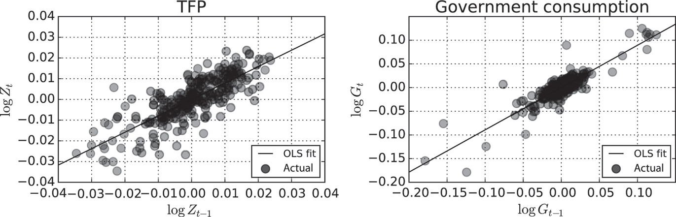
Left panel: Scatter plot of log TFP against log TFP lagged one period. Right panel: Scatter plot of log government consumption against log government consumption lagged one period. Both series are HP-filtered.
We also compute an average ratio of government consumption to GDP of about 20% and we use this value to calibrate the steady state level of government consumption
We use monthly data from June 1964 through November 2017 to compute average values for the inflation rate, the nominal interest rate, and the T-bill rate. We compute an average annual PCE inflation rate of about 3.5% and an average annual 3-month T-bill rate of about 4.9%. So we require that in the steady state gross quarterly inflation Π be about 1.0085 and gross nominal interest Rn be about 1.012. Together these restrictions imply a calibrated value of the household’s subjective discount factor β of about 0.997.
Next, we impose a restriction on the deposit rate. In our model, deposits pay interest and we do not distinguish between different deposit types. However, in practice banks offer several kinds of deposits including demand deposits, small time deposits, and savings account deposits. Historically, Regulation Q in the US prevented banks from offering interest on demand deposits and so an interest rate like the 3-month CD rate will overstate historic interest paid to deposits as a group. Therefore we create a statistic for measuring the average deposit rate taking into account that only a fraction of deposits pay interest.
We measure total deposits as:
and we measure the interest on instruments in M2 minus M1 by the 3-month CD rate. We assume no interest paid on checkable deposits. Our measure of the deposit rate is then given by the weighted average:
Our calculation implies an average annual deposit rate of about 4.5% so we require that the quarterly deposit rate in the model RD equals about 1.011 in the steady state.
From March 2006 to January 2018, the average worker in the US worked about 34.3 hours per week and so we require that the steady state share of household’s available time devoted to labor H equal about 20%. Using quarterly data on outstanding debt and equity of nonfinancial firms in the US, we compute an average leverage ratio for the country of about 29% and we use this to restrict the value of (QK − N)/N. Our value is about 21 percentage points below what BGG use, but the difference has no meaningful effect on our overall calibration and simulated results.
Finally, we compute the average excess reserve to deposit ratio from January 1959 through August 2008 to be 0.051%. We deliberately exclude post-August 2008 data because of the dramatic change in the excess reserve-deposit ratio that began in September 2008. Also, in order to remain consistent in our definition of deposits, we compute this ratio using our measure of total deposits described above and not simply checkable deposits.
In Table 4 we summarize the moments that we use to calibrate the model.
Ten first moments from US data that we use to calibrate ten model parameters.
| Quantity | Model analog | Computed value |
|---|---|---|
| Inflation | Π | 1.00853 |
| Nominal interest (3 mo. T-bills) | Rn | 1.01193 |
| Nominal deposit interest | RD | 1.01098 |
| Investment to GDP ratio | I/Yf | 0.16962 |
| Government consumption to GDP ratio | G/Yf | 0.20457 |
| Annual depreciation to GDP ratio | δK/Yf | 0.13816 |
| Annual GDP growth | ΔYf/Yf | 0.16962 |
| Debt to equity ratio | (K − N)/N | 0.28781 |
| Excess reserves to deposits ratio | Mex/D | 0.00051 |
| Share of time spent working | H | 0.2044 |
B.2 Additional parameter values
We set the Cobb-Douglas production function parameter α to 0.35. We set the elasticity of substitution between retail goods ϵ so that the gross markup of retail goods over wholesale goods is 1.25 Altig et al. (2005). Like SGU, we set the Calvo-pricing parameter θ to 0.8 so that the nominal price of the average retail good remains fixed for 5 quarters. We follow BGG and set ψ – the elasticity of the steady state price of capital Q with respect to the steady state investment to capital ratio – to 0.25. We also follow BBG by setting Ω equal to 0.01 × (1 − α)−1 so that the entrepreneurial wage is 1 percent of output in the steady state.
For the monetary policy rule, we set the coefficient on the lagged nominal interest rate ρr to 0.9, the coefficient on inflation ϕπ to 1.5, and the coefficient on output deviations ϕy/4 to 0.5. Like BGG, we require an annual entrepreneurial default rate of 3%. We accomplish the restriction by setting
Since σσ,t, our shock to the variance of σω,t, does not have a counterpart in CMR – or in any other model of which we are aware – we select an autocorrelation coefficient of 0.9 and suppose a variance 1. We set the banker’s preference parameter ξΦ to 20 for the main simulations and explore in Figure 3 how changing ξΦ affects the predictions of the model.
References
Alloway, T. 2008. “A Tarp Forensic: Fed Funds Rate.” Financial Times.Search in Google Scholar
Altig, D., L. Christiano, M. Eichenbaum, and J. Linde. 2005. “Firm-Specific Capital, Nominal Rigidities and the Business Cycle.” Working Paper 11034, National Bureau of Economic Research, URL http://www.nber.org/papers/w11034.10.3386/w11034Search in Google Scholar
Bernanke, B. S. and M. Gertler. 1989. “Agency Costs, Net Worth, and Busniss Fluctuations.” The American Economic Review 79: 14–31.Search in Google Scholar
Bernanke, B. S., M. Gertler, and S. Gilchrist. 1999. “The Financial Accelerator in a Quantitative Business Cycle Framework.”. In Taylor, J. B., and M. Woodford (Eds.), Handbook of Macroeconomics. Vol. 1C, 1341–1393. Amsterdam: North-Holland.10.1016/S1574-0048(99)10034-XSearch in Google Scholar
Brunnermeier, M. K. 2009. “Deciphering the Liquidity and Credit Crunch 2007–2008.” Journal of Economic Perspectives 23: 77–100.10.1257/jep.23.1.77Search in Google Scholar
Calvo, G. A. 1983. “Staggered Prices in a Utility-Maximizing Framework.” Journal of Monetary Economics 12: 383–398.10.1016/0304-3932(83)90060-0Search in Google Scholar
Canzoneri, M., R. Cumby, B. Diba, and D. López-Salido. 2008. “Monetary Aggregates and Liquidity in a Neo-Wicksellian Framework.” Journal of Money Credit and Banking 40: 1667–1698.10.1111/j.1538-4616.2008.00178.xSearch in Google Scholar
Carlstrom, C. T. and T. S. Fuerst. 1997. “Agency Costs, Net Worth, and Business Fluctuations: A Computable General Equilibrium Analysis.” The American Economic Review 87: 893–910.10.26509/frbc-wp-199602Search in Google Scholar
Christiano, L., R. Motto, and M. Rostagno. 2003. “The Great Depression and the Friedman-Schwartz Hypothesis.” Journal of Money, Credit and Banking 35: 1119–1197.10.1353/mcb.2004.0023Search in Google Scholar
Christiano, L. J., R. Motto, and M. Rostagno. 2014. “Risk Shocks.” American Economic Review 104: 27–65.10.1257/aer.104.1.27Search in Google Scholar
Coval, J., J. Jurek, and E. Stafford. 2009. “The Economics of Structured Finance.” Journal of Economic Perspectives 23: 3–25.10.1257/jep.23.1.3Search in Google Scholar
Dejong, D. N., and C. Dave. 2011. Structural Macroeconometrics. second ed. Princeton: Princeton University Press.10.2307/j.ctt7srm7Search in Google Scholar
Goodfriend, M. and B. T. McCallum. 2007. “Banking and Interest Rates in Monetary Policy Analysis: A Quantitative Exploration.” Journal of Monetary Economics 54: 1480–1507.10.1016/j.jmoneco.2007.06.009Search in Google Scholar
Hart, O. D. and D. M. Jaffee. 1974. “On the Application of Portfolio Theory to Depository Financial Intermediaries.” The Review of Economic Studies 41: 129–147.10.2307/2296404Search in Google Scholar
He, Z. and A. Krishnamurthy. 2013. “Intermediary Asset Pricing.” American Economic Review 103: 732–770.10.1257/aer.103.2.732Search in Google Scholar
Kameník, O. 2011. “Dsge Models with Dynare++. A Tutorial.” Mimeo.Search in Google Scholar
Kane, E. J., and B. G. Malkiel. 1965. “Bank Portfolio Allocation, Deposit Variability, and the Availability Doctrine.” The Quarterly Journal of Economics 79: 113–134.10.2307/1880516Search in Google Scholar
Kashyap, A. K., and J. C. Stein. 1994. “Monetary Policy and Bank Lending.” In Monetary Policy: NBER Studies in Business Cycles, Vol. 29, edited by N. G. Mankiw, 221–256. Chicago: University of Chicago Press.10.3386/w4317Search in Google Scholar
Kashyap, A. K., and J. C. Stein. 2000. “What do a Million Observations on Banks say about the Transmission of Monetary Policy?” The American Economic Review 90: 407–428.10.1257/aer.90.3.407Search in Google Scholar
Krishnamurthy, A., and A. Vissing-Jorgensen. 2013. “Short-Term Debt and Financial Crises: What we can learn from U.S. Treasury Supply.” Upublished Manuscript.Search in Google Scholar
McGrattan, E. R. 1996. “Solving the Stochastic Growth Model with a Finite Element Method.” Journal of Economic Dynamics and Control 20: 19–42.10.1016/0165-1889(94)00842-0Search in Google Scholar
Parkin, M. 1970. “Discount House Portfolio and Debt Selection.” The Review of Economic Studies 37: 469–497.10.2307/2296480Search in Google Scholar
Schmitt-Grohé, S. and M. Uribe. 2006. “Optimal Simple and Implementable Monetary and Fiscal Rules: Expanded Version.” Working Paper 12402, National Bureau of Economic Research, URL http://www.nber.org/papers/w12402.10.3386/w12402Search in Google Scholar
Schmitt-Grohé, S. and M. Uribe. 2007. “Optimal Simple and Implementable Monetary and Fiscal Rules.” Journal of Monetary Economics 54: 1702–1725.10.1016/j.jmoneco.2006.07.002Search in Google Scholar
Sealey, C. W., Jr. 1980. “Deposit Rate-Setting, Risk Aversion, and the Theory of Depository Financial Intermediaries.” The Journal of Finance 35: 1139–1154.10.1111/j.1540-6261.1980.tb02200.xSearch in Google Scholar
©2020 Walter de Gruyter GmbH, Berlin/Boston
Articles in the same Issue
- Contributions
- An empirical study on the New Keynesian wage Phillips curve: Japan and the US
- Risk averse banks and excess reserve fluctuations
- Advances
- Signaling in monetary policy near the zero lower bound
- Contributions
- Robust learning in the foreign exchange market
- Foreign official holdings of US treasuries, stock effect and the economy: a DSGE approach
- Discretion rather than rules? Outdated optimal commitment plans versus discretionary policymaking
- Agency costs and the monetary transmission mechanism
- Advances
- Optimal monetary policy in a model of vertical production and trade with reference currency
- The financial accelerator and marketable debt: the prolongation channel
- The welfare cost of inflation with banking time
- Prospect Theory and sentiment-driven fluctuations
- Contributions
- Household borrowing constraints and monetary policy in emerging economies
- The macroeconomic impact of shocks to bank capital buffers in the Euro Area
- The effects of monetary policy on input inventories
- The welfare effects of infrastructure investment in a heterogeneous agents economy
- Advances
- Collateral and development
- Contributions
- Financial deepening in a two-sector endogenous growth model with productivity heterogeneity
- Is unemployment on steroids in advanced economies?
- Monitoring and coordination for essentiality of money
- Dynamics of female labor force participation and welfare with multiple social reference groups
- Advances
- Technology and the two margins of labor adjustment: a New Keynesian perspective
- Contributions
- Changing demand for general skills, technological uncertainty, and economic growth
- Job competition, human capital, and the lock-in effect: can unemployment insurance efficiently allocate human capital
- Fiscal policy and the output costs of sovereign default
- Animal spirits in an open economy: an interaction-based approach to the business cycle
- Ramsey income taxation in a small open economy with trade in capital goods