Estimating Labor Supply Elasticities in Korea: The Role of Limited Commitment Between Spouses

Seoyoon Jeong; Won Hyeok Kim; Myungkyu Shim

doi:10.1515/bejeap-2024-0254

Article Open Access

Estimating Labor Supply Elasticities in Korea: The Role of Limited Commitment Between Spouses

Seoyoon Jeong , Won Hyeok Kim and Myungkyu Shim

Published/Copyright: March 28, 2025

Published by

Become an author with De Gruyter Brill

Submit Manuscript Author Information Explore this Subject

From the journal The B.E. Journal of Economic Analysis & Policy Volume 25 Issue 2

Abstract

This paper examines if (i) the estimated labor supply elasticity is biased due to changes in the bargaining positions within a household in Korea and (ii) the problem, if detected, can be mitigated by using the distribution of different consumption bundles as a proxy (Bredemeier, Christian, Jan Gravert, and Falko Juessen. 2023. “Accounting for Limited Commitment Between Spouses when Estimating Labor-Supply Elasticities.” Review of Economic Dynamics 51: 547–78). Using KLIPS data from 2008 to 2022, we estimate the Frisch elasticity for married male workers to be around 0.44 and the bias is corrected mostly by controlling for total consumption, not by the distribution of consumption bundles. Similarly, estimates for married female workers did not exhibit significant bias. We suggest possible explanations on why our finding is different from the previous finding using US data.

Keywords: Frisch labor supply elasticity; limited commitment; Korea; KLIPS

JEL Classifications: J12; J16; J22

1 Introduction

Since measuring correct labor supply elasticity is important in both macroeconomics (see Chang and Kim 2006 for related discussions) and microeconomics (see Pencavel 1986 for more discussions), there have been various attempts to identify the sources of biases in estimating the elasticity and to resolve it. For instance, estimates can be biased depending on different household characteristics and preferences over time (Keane and Rogerson 2015): Bredemeier, Gravert and Juessen (2019) showed that ignoring borrowing constraints yields a downward bias in the estimated labor supply elasticities. Bredemeier, Gravert and Juessen (2023) further argued that it is important to consider different bargaining positions within a household by using the distribution of different types of consumption bundles as a proxy for bargaining power when estimating the elasticity because of the limited commitment between married couples.

In this paper, we examine if the recent finding by Bredemeier, Gravert and Juessen (2023) can be applied to the context of South Korea (hereinafter Korea). If married couples have different preferences over different types of consumption goods in the case of Korean households as well, the change in the shares of certain consumption goods bundles at the household level may reflect existing within-household bargaining powers. Therefore, by additionally taking the share of different consumed goods into account, we may be able to mitigate the potential bias in estimating labor supply elasticity in Korea.

Adopting the idea of Bredemeier, Gravert and Juessen (2023) in Korea seems crucial for the following reasons. Korea is a unique country in that despite striving economic development, gender inequality proxied by wage gap and difference in labor market participation rate still prevails.^[1] Panel a of Figure 1 plots the Global Gender Gap Index (GGGI) designed by the World Economic Forum^[2] of Korea (solid blue line), USA (dashed purple line), and the average of OECD countries (dash-dotted green line) from years 2006–2022. Apart from the US or the average of OECD countries, Korea’s GGGI has been below by 0.1 point on average over the years, indicating a consistently low gender equality. Panel b of Figure 1 also shows the gender wage gap of Korea (solid blue line), the US (dashed purple line), and the average of OECD countries (dash-dotted green line) over the years from 1999 to 2022. While the overall trend indicates a declining wage gap in Korea, it is still apparently wide compared to other developed countries. Therefore, considering possible changes in bargaining positions within a household for a country with high levels of gender inequality as in Korea seems meaningful.

Figure 1:

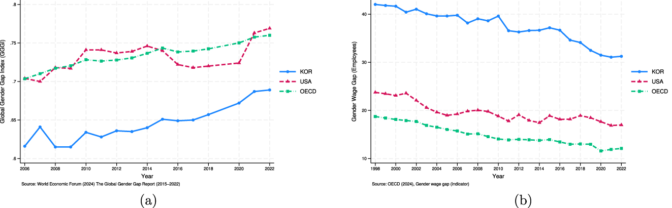
Comparing gender inequality in Korea with the US and OECD countries. (a) Global gender gap index. (b) Gender wage gap.

To estimate the Frisch elasticity in Korea that takes limited commitment between spouses into account, we use the Korean Labor and Income Panel Study (KLIPS) data, a panel survey on Korean households that contains information on various individual and household characteristics including individual-level income and working hours, along with household-level consumption patterns. Using data from 2008 to 2022, we estimate a labor supply equation that considers total consumption at the household level and different types of consumption bundles as a proxy for within-household bargaining powers under a two-way time and individual fixed effects model with different taste shifters. We find that the estimated Frisch elasticity increases mainly when aggregate consumption is controlled for but the bias correction due to controlling for different consumption bundle shares does not seem sizable, a finding inconsistent with Bredemeier, Gravert and Juessen (2023); on average 0.05 more in magnitude for men when aggregate consumption is controlled, while the overall bias was not significant for women. Specifically, the elasticity is estimated to be around 0.44 for married employed men and 0.49 for married employed women. Additional subgroup analyses based on various individual and household characteristics confirm that our main finding is robust: Subgroups by age, education level, type of employment status, single- or dual-earner households, and the presence of children also show overall bias easing when the aggregate consumption is controlled while such an effect does not prevail when controlling for consumption bundles, with the younger, less educated, temporary workers along with households of single-earners and with no children being slightly more elastic. We further show that deflating each consumption bundle by its own price level, which was not considered in Bredemeier, Gravert and Juessen (2023), does not change our finding.

In sum, unlike the US, Korean data show that considering additional controls for consumption bundles does not further mitigate downward bias in Frisch elasticity. We suggest that this may be due to the lack of explanatory power of household consumption patterns on bargaining powers of Korean households, and examine the relationship between household consumption bundle shares and other well-known bargaining power indicators such as share of earnings/wages and housework contribution hours. We find a weakly negative (resp. positive) relationship between the share of male labor income or wage (resp. male housework hours) and the share of food consumption of households, which implies that relatively more bargaining power of male household members does not correlate with more consumption in food for Korean households. Analysis with service consumption of households yields similar results.

This paper contributes to the literature in several dimensions. First, we provide an unbiased estimate of the Frisch elasticity in Korea in that limited commitment and different bargaining positions over time are considered, which to our knowledge is hardly done using Korean data. In the sense that they estimated the labor supply elasticity in Korea, Moon and Song (2016) and Kim, Shim and Yang (2022) are close to our paper. Moon and Song (2016) estimated the micro labor supply elasticity of Korea to be around 0.23 by using the KLIPS survey data from 2000 to 2008. Kim, Shim and Yang (2022) estimated the Frisch elasticity in Korea for men when borrowing constraint within a household is controlled, inferring an existence of a downward bias without such consideration. While both papers estimate for Korea’s labor supply elasticity, neither have considered the composition of consumption goods of households. Second, this paper constructs different types of consumption bundles using Korean data and finds that while they can be a proxy for bargaining powers of spouses in certain settings such as the US, consumption patterns showing bargaining power may not be for all countries. Our estimation results suggest that information on the different shares of consumption bundles may not accurately reflect different bargaining positions between spouses in the case of Korea, a country in which persistent gender wage and economic participation gap is observed.

This paper is organized as follows. Section 2 briefly introduces the model developed by Bredemeier, Gravert and Juessen (2023) and the empirical methodology behind the analysis. Empirical results are presented in Section 3. Finally, Section 4 concludes.

2 Empirical Strategy

2.1 A Labor Supply Model with Limited Commitment

In this section, we briefly discuss the labor supply model in Bredemeier, Gravert and Juessen (2023) that considers limited commitment and endogenous divorce in households.^[3] Individuals maximize their expected lifetime utility by drawing utility from consumption, the quality of marriage, and disutility from work. Men and women differ in their preference over different types of consumption goods and always have the outside option to leave the marriage at anytime. Since enforcing the other spouse to stay married is impossible, commitment between spouses is limited. Using the partial equilibrium life cycle labor supply model with household consumption bundle shares considered as a proxy for limited commitment, Bredemeier, Gravert and Juessen (2023) derive the following equation, which can correct the bias from ignoring the limited commitment problem:

(2.1) log h g j , t = η g ⋅ log w g j , t ︸ A − η g σ g ⋅ log c ̃ j , t ︸ B − η g σ g ( γ g − γ − g ) c ̄ k c ̄ g log ( c ̃ j , k , t / c ̃ j , t ) ︸ C − η g ⋅ ( 1 − σ g Θ 2 + σ g ) ⋅ log P g , t − η g σ g Θ 3 log P − g , t + η g σ g Θ 1 log p k , t − η g ⋅ log α g j , t + Θ 0

where

Θ g , 0 = c ̄ k / c ̄ g log ( c ̄ k / c ̄ ) / ( γ − g , k − γ g , k ) + log ( c ̄ g / c ̄ ) , Θ g , 1 = c ̄ k / c ̄ g / ( γ − g , k − γ g , k ) , Θ g , 2 = ( ν − 1 ) γ g , k / ( γ − g , k − γ g , k ) , Θ g , 3 = ( ν − 1 ) γ − g , k c ̄ − g / c ̄ g / ( γ − g , k − γ g , k ) .

Here g ∈ {m, f} denotes the individual’s gender (male (m), or female (f)), with −g denoting the opposite gender, j denotes the household she lives in, h _gj,t her hours worked, α _gj,t her preference for work, and w _gj,t her wage rate. c ̃ j , t indicates the total household level consumption while c ̃ j , k , t is the household level consumption of goods bundle k. Note that γ _g,k is the individual’s preference weight on consumption bundle k and P _g,t is the aggregate price of the gender-specific consumption bundle, indicating that agents have different preferences over different consumption goods. σ _g is the rate of risk aversion and the elasticity of substitution between bundles is denoted as ν and η _g is the Frisch elasticity of labor supply for each individual g.

All variables in the first line of equation (2.1) are observable, implying that we can directly estimate the Frisch labor supply elasticity without bias using the data. We note that the first term (A) on the right-hand side of the equation captures the substitution effect of an increase in wage rate on hours worked, while the second term (B) controls for the wealth effect by considering the total level of goods consumed at the household level. The third term (C) is what captures the bias from limited commitment between spouses, which has been neglected by previous literature. Given that there exists a difference in the preference weight of certain goods between spouses, in other words, γ _f,k ≠ γ _m,k, the share of consumption on goods bundle k reflects spouses’ varying bargaining power. This can be implied through the idea that as one’s bargaining power rises within the household, it is more likely for that household to consume on goods that individual prefers. Controlling for this would let us exclude the bargaining effect on the labor supply.

The remaining variables in the second and third lines either do not vary across households or over time, letting an unbiased Frisch elasticity estimation be available under a two-way individual and time fixed effect analysis.

2.2 Empirical Analysis

2.2.1 Methodology

For the empirical analysis, we mainly estimate equation (2.1), but with few adjustments. First, we estimate with log-differenced data instead of estimating the equation with log-level data.^[4] In other words, we regress hours growth on expected wage growth, to strengthen the property of leaving the marginal utility of wealth constant (see Altonji 1986; Bredemeier, Gravert and Juessen 2019).^[5] This modification also allows to compare estimation results to previous literature as most papers using Korean data uses the log-differenced data to estimate the labor supply elasticity of Korea.^[6] We estimate with individual and time fixed effects to take the variables in the second and third line of equation (2.1), which are either non-time or -individual varying, into account. Altogether, we estimate the following equation:

(2.2) Δ log h g j , t = η g E t Δ log w g j , t + Γ j Δ log C j , t + δ g j , t + χ g , t + μ g j + ϵ g j , t

where Δlogx _t = logx _t+1 − logx _t for any variable x _t, C _j,t is a vector of consumption-related variables including c ̃ j , t and c ̃ j , k , t / c ̃ j , t for all k = 1, …, K, δ _gj,t is a set of observable taste shifters such as age and the number of children, and χ _g,t and μ _gj are time and individual fixed effects, respectively.

It is well known that simply using wage rates computed as earnings over hours worked for labor supply regression causes a measurement error to bias estimates toward zero (see Altonji 1986; Keane 2011). Therefore, running an initial wage regression to predict the expected wage growth, E _tΔlogw _gj,t, is necessary (Borjas 1980). Similar to Bredemeier, Gravert and Juessen (2023), we run a first-stage wage regression on the actual wage growth rate that includes a third-order polynomial in age and interactions with education,^[7] year dummies, and other variables including taste shifters such as the number of young and old children. Moreover, as suggested in Moon and Song (2016) and Domeij and Floden (2006), we also account for a lag of the log wage rate to resolve additional endogeneity issues.^[8]

2.2.2 Data

We use the KLIPS data from 2008 to 2022 for the empirical analysis.^[9] The main survey is conducted annually on a sample of 5,000 urban households in Korea on various information including household characteristics, economic activities, income, expenditure, and more.^[10] This survey especially allows to decompose household expenditures into different types of goods and services, which is key in estimating the Frisch elasticity while taking into account the relative bargaining positions and limited commitment within households. For the main analysis we consider married households where the head is aged 25–60 and is currently an employed worker.^[11] The same standard is applied for the spouses when estimating for women, which is discussed later in detail. We trim top and bottom 1 % of the data based on the growth rate of log wage and hours worked to exclude extreme outliers.^[12]

The working hours variable is constructed by adding average regular and overtime hours worked per week. Monthly post-tax labor earnings in Korean won are deflated using the Consumer Price Index (2020 = 100) data from the KOrean Statistical Information Service (KOSIS). The hourly wage rate is thus calculated by dividing monthly earnings by monthly hours worked.

KLIPS provides monthly average consumption data on 20 categories of consumption goods and services for a given household. Closely following the consumption item mapping of Bredemeier, Gravert and Juessen (2023), we utilize the 10 consumption bundles shown in Table 1. Note that some categories such as specific housing utility expenses are directly unavailable in the dataset, so some adjustments are made to include them in the estimation. Under the housing maintenance expenses category are included electricity, water, heating, and rent expenditures. Bredemeier, Gravert and Juessen (2023) excluded rent-equivalent variables as it also interacts with bargaining positions and commitment problems in a form of wealth, apart from different consumption preferences among spouses, which is the main channel this estimation focuses on. However, the KLIPS data for housing maintenance expenses includes all the main housing utility expenses, which consists most of the non-food category of the consumption items. Hence, we modify the variable by manually excluding rent if the household is living under rent or other equivalent situations.^[13] All categories are expressed as monthly consumption levels in Korean won.

Table 1:

Categorization of KLIPS consumption items.

Item	Category
Food and groceries	Food
Meals out	Food
Public education	Services
Private education	Services
Vehicle maintenance expenses	Services
Public transportation	Services
Health and medical costs	Services
Medical insurance	Services
Expenses for communication	Non-food
Housing maintenance expenses	Non-food

In this empirical analysis, three approaches are implemented in using the consumption variables as a proxy for within household bargaining power. First, consumption items are aggregated into three categories: food, services, and non-food expenditures.^[14] We then apply the expenditure share of food and services accordingly as control variables. Second, principal components of the shares of all 10 items are considered. Lastly, all of the shares of 10 items are included. We note that in all three specifications, the total household consumption calculated as the sum of all consumption bundles are included.

A time fixed effect in equation (2.2) allows the regression to filter out price effects and other fluctuations caused by business cycles. A third-order polynomial in age and the number of children in the household are added as time varying taste shifters.^[15] Table 2 shows the summary statistics of the main variables mentioned earlier.

Table 2:

Summary statistics.

Variable	Observations	Mean	SD	Min	Max
Monthly hours worked	30,199	186.8	35.1	9	421
Monthly labor income (10,000 won)	30,142	365.9	179.9	0	6,736
Monthly avg. total consumption (10,000 won)	30,091	219.8	91.8	0	1,196
Monthly avg. food consumption (10,000 won)	30,091	72.8	30.5	0	353
Monthly avg. service consumption (10,000 won)	30,091	109.0	69.1	0	898
Monthly avg. non-food consumption (10,000 won)	30,091	37.9	13.1	0	389

Note: Data from KLIPS data. Monthly hours worked and labor income reported are of male heads only.

3 Empirical Results

3.1 Main Analysis

The main results are presented in Table 3. Column (1) refers to a simple regression where hours growth rate is regressed on predicted wage growth rate with time and individual fixed effects along with other control variables such as age and number of children. This regression is unable to identify Frisch elasticity correctly as consumption, or wealth, is not held constant, hence the income effect is not taken into account. The second column shows that the elasticity increases from 0.378 to 0.431 when total household consumption is considered, thus in line with Altonji (1986).

Table 3:

Labor supply elasticity for men.

	(1)	(2)	(3)	(4)	(5)	(6)	(7)
Log wage growth rate	0.378^***	0.431^***	0.435^***	0.435^***	0.436^***	0.436^***	0.435^***
Δ log w ̃ m j , t	(0.0191)	(0.0201)	(0.0201)	(0.0201)	(0.0202)	(0.0202)	(0.0202)
Log total consumption growth		−0.039^***	−0.042^***	−0.040^***	−0.038^***	−0.038^***	−0.038^***
Δ log c ̃ j , t		(0.0046)	(0.0048)	(0.0049)	(0.0047)	(0.0048)	(0.0051)
Log food share growth			−0.010^***
Δ log ( c ̃ j , t , F / c ̃ j , t )			(0.0038)
Log service share growth				0.002
Δ log ( c ̃ j , t , S / c ̃ j , t )				(0.0037)
1st principle component					−0.002	−0.002
					(0.0020)	(0.0022)
2nd pc	No	No	No	No	No	Yes	No
3rd pc	No	No	No	No	No	Yes	No
All consumption shares	No	No	No	No	No	No	Yes
R ²	0.109	0.114	0.115	0.114	0.115	0.115	0.116
Number of HH	2,536	2,536	2,536	2,536	2,534	2,534	2,534
Observations	14,238	14,238	14,238	14,238	14,202	14,202	14,202

Note: Dependent variable is log hours worked growth Δlogh _mj,t. Standard errors in parentheses (^*** p < 0.01, ^** p < 0.05, ^* p < 0.1). All regressions control for individual and time fixed effects, a cubic in age, range of children (0/1–2/3−) and education of head (high school or less/college/grad school and up).

However, as mentioned earlier, coefficient of column (2) may still be biased downwards due to limited commitment among spouses in a household (Bredemeier, Gravert and Juessen 2023). The third column shows the estimate for the elasticity when adding share of food consumption as another control variable. The elasticity slightly increases to 0.435, which is approximately 0.004 larger than the case where only total household consumption is considered. Note that the estimated coefficient on the food consumption share is negative, which implies that food may be goods preferred more by men than women, which is in line with what the limited commitment theory predicts (see Mazzocco 2007). Similarly, column (4) switches out share of food consumption to share of services consumption, which gives the same level of elasticity (0.435) as in column (3). Columns (5) and (6) control for the first and second and third principal components, respectively. These also result in a similar magnitude of estimates for the elasticity, around 0.436. Lastly, column (7) considers all 10 shares of consumption separately, in which leads to an estimate around 0.435.

In sum, we find that signs of the estimates for each consumption bundles (food and services) are in line with Bredemeier, Gravert and Juessen (2023). For instance, the negative estimated coefficient for food share shows some evidence that food consumption provides somewhat more utility to men than women in Korea as well. However, the bias from omitted variables problem seems to be much less severe in Korea than in the US. Specifically, in Bredemeier, Gravert and Juessen (2023), the Frisch labor supply elasticity is only 0.23 when wealth is not controlled for, 0.45 when only total household consumption is controlled for and ranges from 0.63 to 0.66 when adding different consumption shares into the regression. In contrast, the jump from 0.378 to 0.431 in columns (1) and (2) and almost no change between column (2)–(3) indicate that controlling total consumption alone can mitigate the downward bias of the elasticity in Korea.

Table 4 shows results for married, employed women aged 25–60. In line with the literature, estimated Frisch labor supply elasticities for women are larger than that for men when consumption is not controlled for. The estimated Frisch elasticity tends to increase as information on total household consumption and different consumption shares are considered, but this change is minuscule: The estimate for elasticity when consumption is not considered at all is 0.471 (column (1)), while controlling for total consumption gives an estimation of 0.485 (column (2)). Thus we can conclude that the downward bias is not as substantial for women than in men. This could be due to several constraints: The number of observations for working women is roughly half that of men and important factors that affect labor participation of women such as home production rate are excluded from the estimation. The estimated coefficient for food consumption share is also negative for women, although statistically insignificant, which may imply that consumption preference between spouses are not as apparent in Korea as in the US.

Table 4:

Labor supply elasticity for women.

	(1)	(2)	(3)	(4)	(5)	(6)	(7)
Log wage growth rate	0.471^***	0.485^***	0.485^***	0.484^***	0.480^***	0.480^***	0.478^***
Δ log w ̃ m j , t	(0.0410)	(0.0413)	(0.0413)	(0.0413)	(0.0414)	(0.0414)	(0.0415)
Log total consumption growth		−0.021^***	−0.021^***	−0.016^*	−0.024^***	−0.025^***	−0.019^**
Δ log c ̃ j , t		(0.0078)	(0.0081)	(0.0085)	(0.0080)	(0.0081)	(0.0088)
Log food share growth			−0.002
Δ log ( c ̃ j , t , F / c ̃ j , t )			(0.0068)
Log service share growth				−0.010
Δ log ( c ̃ j , t , S / c ̃ j , t )				(0.0079)
1st principle component					0.006^*	0.005
					(0.0036)	(0.0040)
2nd pc	No	No	No	No	No	Yes	No
3rd pc	No	No	No	No	No	Yes	No
All consumption shares	No	No	No	No	No	No	Yes
R ²	0.139	0.140	0.140	0.140	0.140	0.140	0.140
Number of HH	1,374	1,374	1,374	1,374	1,374	1,374	1,374
Observations	7,186	7,186	7,186	7,186	7,175	7,175	7,175

Note: Dependent variable is log hours worked growth Δlogh _fj,t. Standard errors in parentheses (^*** p < 0.01, ^** p < 0.05, ^* p < 0.1). All regressions control for individual and time fixed effects, a cubic in age, range of children (0/1–2/3−) and education of head (high school or less/college/grad school and up).

3.2 Additional Analysis

The main findings show that although bias is corrected when using the distribution of different types of consumption bundles, it is not as clear nor significant in magnitude in Korea. Still, it is noteworthy that the additional control for household consumption eases the downward bias by around 0.057 for employed men. In this section, we examine if our main finding is robust.

As a first robustness check, we run an alternative regression where we control for household asset and debt levels instead of consumption in attempts to hold marginal utility of wealth constant and compare the estimated Frisch elasticities with those when consumption is held constant. We then further conduct several subgroup analyses as in Bredemeier, Gravert and Juessen (2023) by dividing employed men into various subgroups while including additional subgroups of our own: (1) by age groups, (2) by education level, (3) by employment status, (4) by single- or dual-earner positions, and (5) by existence of children.^[16] As the predicted wage rate is based on the interaction between age and education, Bredemeier, Gravert and Juessen (2023) estimates elasticities per subgroups of these determinants. We look into further subgroups based on individual characteristics that might matter in the Korean setting. Lastly, we check robustness of our findings by deflating each consumption bundle by its own price level rather than deflating by aggregate CPI.

3.2.1 Labor Supply Elasticity with Household Asset and Debt

We first report the results of different proxies for wealth in Table 5. Columns (2) through (4) are equivalent to the results reported in Table 3 columns (1) through (3). Column (1) refers to the estimated elasticity when hours growth rate is regressed on predicted wage growth rate with a time fixed effect and the same control variables as in the main analysis, with the addition of controlling household asset growth and debt differences instead of consumption. We note that the coefficient estimates in columns (1) (0.421) and (3) (0.431) do not differ in magnitude. In other words, controlling for household financial asset and debt can also alleviate the downward bias coming from the wealth effect alike controlling for household total consumption. This infers that when consumption data is assumed to be non-reliable due to various measurement errors, capturing the wealth effect by controlling for other variables that are less likely to have observation noise, such as asset and debt, also gives similar results.

Table 5:

Labor supply elasticity for men: controlling wealth effect.

	Asset	Consumption
	(1)	(2)	(3)	(4)
Log wage growth rate	0.421^***	0.378^***	0.431^***	0.435^***
Δ log w ̃ m j , t	(0.0197)	(0.0191)	(0.0201)	(0.0201)
Log total consumption growth			−0.039^***	−0.042^***
Δ log c ̃ j , t			(0.0046)	(0.0048)
Log food share growth				−0.010^***
Δ log ( c ̃ j , t , F / c ̃ j , t )				(0.0038)
Log financial asset growth	0.001^***
Δ log asset ̃ FIN,jt	(0.0002)
Log real estate asset growth	−0.000
Δ log asset ̃ EST,jt	(0.0002)
Log debt growth	0.000
Δ log debt ̃ j t	(0.0001)
R ²	0.114	0.109	0.114	0.115
Number of HH	2,536	2,536	2,536	2,536
Observations	14,238	14,238	14,238	14,238

Note: Dependent variable is log hours worked growth Δlogh _mj,t. Standard errors in parentheses (^*** p < 0.01, ^** p < 0.05, ^* p < 0.1). All regressions control for individual and time fixed effects, a cubic in age, range of children (0/1–2/3−) and education of head (high school or less/college/grad school and up).

3.2.2 Subgroup Analysis

In this section, we conduct a battery of robustness checks based on various subgroups. First, samples are divided into two groups based on age because severity of the limited commitment problem might be age-dependent: age of young ranges from 25 to 39 and old ranges from 40 to 60. Table 6 shows results for young and the old, in which similar patterns of increasing estimated elasticities when consumption is accounted for is observed: Estimates change from 0.456 (column (1)) to 0.532 (column (2)) and 0.362 (column (4)) to 0.410 (column (5)) for young and old, respectively. Adding food consumption share into the equation slightly increases the estimated coefficient, but only by less than 0.04 for both groups. Comparing the estimates between the subgroups, younger workers have slightly higher estimates, but this difference is not that significant, which is in contrast with the case for the US.^[17]

Table 6:

Labor supply regressions for age subgroups of men.

	Young (25–39)			Old (40–60)
	(1)	(2)	(3)	(4)	(5)	(6)
Log wage growth rate	0.456^***	0.532^***	0.535^***	0.362^***	0.410^***	0.414^***
Δ log w ̃ m j , t	(0.0367)	(0.0383)	(0.0384)	(0.0232)	(0.0244)	(0.0244)
Log total consumption growth		−0.058^***	−0.060^***		−0.034^***	−0.038^***
Δ log c ̃ j , t		(0.0090)	(0.0093)		(0.0056)	(0.0058)
Log food share growth			−0.007			−0.011^**
Δ log ( c ̃ j , t , F / c ̃ j , t )			(0.0073)			(0.0045)
R ²	0.163	0.176	0.176	0.113	0.117	0.118
Number of HH	890	890	890	2,014	2,014	2,014
Observations	3,702	3,702	3,702	10,292	10,292	10,292

Note: Dependent variable is log hours worked growth Δlogh _mj,t. Standard errors in parentheses (^*** p < 0.01, ^** p < 0.05, ^* p < 0.1). All regressions control for individual and time fixed effects, a cubic in age, range of children (0/1–2/3−) and education of head (high school or less/college/grad school and up).

Secondly, samples are also divided into two groups based on their education level as different education level might affect perceptions on gender inequality and labor supply behavior: low education level for those up to high school graduates and high for those college graduates and up. Results are presented in Table 7. The effect of taking consumption into account through the addition of food consumption share can also be found for the two educational subgroups: The Frisch elasticity of high school graduates or less increases from 0.474 (column (1)) to 0.556 (column (2)) when total household consumption is added and 0.561 (column (3)) when the food expenditure share is additionally controlled for. The estimated elasticity of college graduates or more also increases from 0.306 (column (4)) to 0.340 (column (5)) and up to 0.343 (column (6)) when food share is also considered. Comparing the two groups based on education level, estimated labor supply elasticity seems slightly higher for lower educated men, however the difference cannot be said significant.

Table 7:

Labor supply regressions for education subgroups of men.

	Low (high school graduates)			High (college graduates)
	(1)	(2)	(3)	(4)	(5)	(6)
Log wage growth rate	0.474^***	0.556^***	0.561^***	0.306^***	0.340^***	0.343^***
Δ log w ̃ m j , t	(0.0363)	(0.0383)	(0.0385)	(0.0206)	(0.0215)	(0.0216)
Log total consumption growth		−0.057^***	−0.060^***		−0.026^***	−0.029^***
Δ log c ̃ j , t		(0.0088)	(0.0091)		(0.0050)	(0.0051)
Log food share growth			−0.010			−0.010^**
Δ log ( c ̃ j , t , F / c ̃ j , t )			(0.0075)			(0.0039)
R ²	0.119	0.127	0.128	0.099	0.103	0.104
Number of HH	964	964	964	1,572	1,572	1,572
Observations	5,358	5,358	5,358	8,878	8,878	8,878

Note: Dependent variable is log hours worked growth Δlogh _mj,t. Standard errors in parentheses (^*** p < 0.01, ^** p < 0.05, ^* p < 0.1). All regressions control for individual and time fixed effects, a cubic in age, range of children (0/1–2/3−) and education of head (high school or less/college/grad school and up).

Apart from Bredemeier, Gravert and Juessen (2023), we additionally conduct several subgroup estimations based on whether (1) individuals are regularly employed or not, (2) households are single- or dual-earners, and (3) households have children or not. Regular employment is defined as employment of full-time workers directly hired by employers without a fixed-term contract and is generally known for having higher job security. Others including temporary workers under a fixed-term contract or dispatched and subcontracted workers are classified as temporary workers. Single-earner households are those where the male head is the only person who earns labor income while dual-earner households are those where both spouses earn labor income.

The rise of temporary employment contracts has appeared worldwide since the 1990s. While many countries do not face much conflict, the apparent differences and discrimination between regular and temporary employments has been an on-going social conflict in Korea (see Moon 2014). Hence, we subgroup individuals by regular and temporary employment status to identify if differences in terms of labor supply elasticity also exists among the two groups. According to Table 8, both groups still hold the effect of increased estimated elasticities when total household consumption and food consumption share are accounted for the regression. Although estimated elasticity values slightly differ between the two groups, it is hard to say that they are significantly different. In addition, due to a large difference in sample size between the two groups, inferring further interpretation is limited.

Table 8:

Labor supply regressions for employment status subgroups of men.

	Regular worker			Temporary worker
	(1)	(2)	(3)	(4)	(5)	(6)
Log wage growth rate	0.379^***	0.422^***	0.426^***	0.421^***	0.513^***	0.511^***
Δ log w ̃ m j , t	(0.0188)	(0.0198)	(0.0198)	(0.0712)	(0.0742)	(0.0746)
Log total consumption growth		−0.031^***	−0.035^***		−0.072^***	−0.070^***
Δ log c ̃ j , t		(0.0046)	(0.0047)		(0.0170)	(0.0181)
Log food share growth			−0.013^***			0.005
Δ log ( c ̃ j , t , F / c ̃ j , t )			(0.0036)			(0.0157)
R ²	0.116	0.120	0.121	0.126	0.137	0.137
Number of HH	2,172	2,172	2,172	419	419	419
Observations	12,185	12,185	12,185	1,923	1,923	1,923

Note: Dependent variable is log hours worked growth Δlogh _mj,t. Standard errors in parentheses (^*** p < 0.01, ^** p < 0.05, ^* p < 0.1). All regressions control for individual and time fixed effects, a cubic in age, range of children (0/1–2/3−) and education of head (high school or less/college/grad school and up).

As some literature such as in Yogev and Brett (1985) suggest in observing spouses’ involvement in family roles based on dual- and single-earner couples, we also analyze if any difference in terms of labor supply elasticity exists between households of single-earner and dual-earner and report the results under Table 9. Note that we only account for households where the male head is the single-earner for single-earner households. Although we find similar effects of increased estimated elasticities when consumption variables are additionally controlled for the regression, no distinct differences between the subgroups are to be found.

Table 9:

Labor supply regressions for dual- or single-earner subgroups of men.

	Dual earner household			Single earner household (by male)
	(1)	(2)	(3)	(4)	(5)	(6)
Log wage growth rate	0.353^***	0.412^***	0.417^***	0.398^***	0.446^***	0.448^***
Δ log w ̃ m j , t	(0.0275)	(0.0291)	(0.0292)	(0.0281)	(0.0293)	(0.0294)
Log total consumption growth		−0.040^***	−0.045^***		−0.039^***	−0.041^***
Δ log c ̃ j , t		(0.0067)	(0.0069)		(0.0069)	(0.0071)
Log food share growth			−0.013^**			−0.006
Δ log ( c ̃ j , t , F / c ̃ j , t )			(0.0054)			(0.0056)
R ²	0.141	0.147	0.148	0.130	0.135	0.135
Number of HH	1,407	1,407	1,407	1,431	1,431	1,431
Observations	6,894	6,894	6,894	6,873	6,873	6,873

Note: Dependent variable is log hours worked growth Δlogh _mj,t. Standard errors in parentheses (^*** p < 0.01, ^** p < 0.05, ^* p < 0.1). All regressions control for individual and time fixed effects, a cubic in age, range of children (0/1–2/3−) and education of head (high school or less/college/grad school and up).

Lastly, labor supply elasticity is separately estimated based on the presence of children within the household. Although we have controlled for the range of number of children in our previous regressions, households without children may have different consumption patterns with those who have children. While children were merely accounted for when observing family behaviors in past economic literature, recent marketing studies emphasize the importance of children in family decision making, especially in the context of household consumption (see Berey and Pollay 1968; Dauphin et al. 2011 for related discussions). Table 10 shows that households have increased estimates when total consumption and food consumption share are controlled for, regardless of the existence of children. Estimated values slightly differ between the two groups, but the magnitude and direction of the increased estimates are fairly similar.

Table 10:

Labor supply regressions for presence of children subgroups of men.

	One or more children			No children
	(1)	(2)	(3)	(4)	(5)	(6)
Log wage growth rate	0.366^***	0.423^***	0.428^***	0.425^***	0.475^***	0.477^***
Δ log w ̃ m j , t	(0.0218)	(0.0229)	(0.0229)	(0.0421)	(0.0445)	(0.0446)
Log total consumption growth		−0.045^***	−0.048^***		−0.033^***	−0.035^***
Δ log c ̃ j , t		(0.0055)	(0.0056)		(0.0095)	(0.0099)
Log food share growth			−0.011^**			−0.005
Δ log ( c ̃ j , t , F / c ̃ j , t )			(0.0043)			(0.0083)
R ²	0.108	0.115	0.116	0.138	0.142	0.142
Number of HH	1,898	1,898	1,898	845	845	845
Observations	10,345	10,345	10,345	3,684	3,684	3,684

Note: Dependent variable is log hours worked growth Δlogh _mj,t. Standard errors in parentheses (^*** p < 0.01, ^** p < 0.05, ^* p < 0.1). All regressions control for individual and time fixed effects, a cubic in age, and education of head (high school or less/college/grad school and up).

3.2.3 Considering CPI by Items for Consumption Bundle Data

As some consumption goods may have relatively different CPI levels, we also consider deflating each consumption bundle consumed by its own price level rather than by the aggregate CPI. We use the CPI by item data from KOSIS between 2007 and 2021. The following Table 11 displays the types of CPI by item categories considered when we deflate the corresponding consumption bundle price for each household in each year.

Table 11:

List of CPI by item for corresponding KLIPS consumption items.

Item	CPI by item (KOSIS)
Food and groceries	Food and non-alcoholic beverages
Meals out	Catering services
Public education	Education
Private education	Education
Vehicle maintenance expenses	Operation of personal transport equipment
Public transportation	Passenger transport by road
Health and medical costs	Health
Medical insurance	Health
Expenses for communication	Communication
Housing maintenance expenses	Housing, water, electricity and other fuels

Table 12 shows the labor supply regression results for men when we deflate consumption goods by its own price levels. Comparing the results to our main regression results, estimated coefficients hardly differ whether we deflate consumption goods by its own price levels or an aggregated price level. As in the main regression results, most of the downward bias is mitigated when we consider the aggregate household consumption.

Table 12:

Labor supply elasticity for men when deflated with item-level CPI.

	(1)	(2)	(3)	(4)	(5)	(6)	(7)
Log wage growth rate	0.378^***	0.432^***	0.435^***	0.436^***	0.436^***	0.436^***	0.435^***
Δ log w ̃ m j , t	(0.0191)	(0.0201)	(0.0201)	(0.0201)	(0.0202)	(0.0202)	(0.0202)
Log total consumption growth		−0.039^***	−0.042^***	−0.040^***	−0.038^***	−0.038^***	−0.037^***
Δ log c ̃ j , t		(0.0046)	(0.0048)	(0.0049)	(0.0047)	(0.0048)	(0.0051)
Log food share growth			−0.009^**
Δ log ( c ̃ j , t , F / c ̃ j , t )			(0.0038)
Log service share growth				0.001
Δ log ( c ̃ j , t , S / c ̃ j , t )				(0.0036)
1st principle component					−0.002	−0.002
					(0.0020)	(0.0022)
2nd pc	No	No	No	No	No	Yes	No
3rd pc	No	No	No	No	No	Yes	No
All consumption shares	No	No	No	No	No	No	Yes
R ²	0.109	0.114	0.114	0.114	0.115	0.115	0.116
Number of HH	2,536	2,536	2,536	2,536	2,534	2,534	2,534
Observations	14,238	14,238	14,238	14,238	14,202	14,202	14,202

Note: Dependent variable is log hours worked growth Δlogh _mj,t. Standard errors in parentheses (^*** p < 0.01, ^** p < 0.05, ^* p < 0.1). All regressions control for individual and time fixed effects, a cubic in age, range of children (0/1–2/3−) and education of head (high school or less/college/grad school and up).

Similar results are found for Frisch elasticity estimates for women. Table 13 shows the regression results for women while using information on CPI by item. We find that considering specific price levels by items for the consumption data gives results consistent with the main regression for women as well.

Table 13:

Labor supply elasticity for women when deflated with item-level CPI.

	(1)	(2)	(3)	(4)	(5)	(6)	(7)
Log wage growth rate	0.471^***	0.485^***	0.485^***	0.484^***	0.480^***	0.480^***	0.479^***
Δ log w ̃ m j , t	(0.0410)	(0.0413)	(0.0413)	(0.0413)	(0.0414)	(0.0414)	(0.0415)
Log total consumption growth		−0.022^***	−0.022^***	−0.017^**	−0.025^***	−0.025^***	−0.020^**
Δ log c ̃ j , t		(0.0079)	(0.0081)	(0.0085)	(0.0080)	(0.0081)	(0.0088)
Log food share growth			−0.001
Δ log ( c ̃ j , t , F / c ̃ j , t )			(0.0070)
Log service share growth				−0.012
Δ log ( c ̃ j , t , S / c ̃ j , t )				(0.0076)
1st principle component					0.006^*	0.005
					(0.0036)	(0.0040)
2nd pc	No	No	No	No	No	Yes	No
3rd pc	No	No	No	No	No	Yes	No
All consumption shares	No	No	No	No	No	No	Yes
R ²	0.138	0.140	0.140	0.140	0.140	0.140	0.140
Number of HH	1,374	1,374	1,374	1,374	1,374	1,374	1,374
Observations	7,186	7,186	7,186	7,186	7,175	7,175	7,175

Note: Dependent variable is log hours worked growth Δlogh _fj,t. Standard errors in parentheses (^*** p < 0.01, ^** p < 0.05, ^* p < 0.1). All regressions control for individual and time fixed effects, a cubic in age, range of children (0/1–2/3−) and education of head (high school or less/college/grad school and up).

3.3 Bargaining Powers and Consumption Patterns within South Korean Households

In summary, our analyses show that while controlling for consumption partially mitigates the downward bias, adding additional controls for consumption bundles does not clearly affect bias correction in magnitude, a finding inconsistent with that of the US. In this section, we argue that such a conclusion can be explained by the fact that bargaining powers within a Korean household may not be clearly reflected in household consumption patterns. In order to examine this to a certain extent, we attempt in looking into the relationship between household consumption bundle shares and other bargaining power indicators. Although there is no consensus in the literature on how to measure intra-household bargaining power, there have been several attempts to do so. Some literature use the share of annual earnings (see Bittman et al. 2003; Geist 2005) to measure the power a spouse has in the household where the spouse who earns more of the total household earning has more power. Other papers focus on the time allocation to housework of spouses. Typically, housework contribution and bargaining power within the household are negatively related (see Bittman et al. 2003; Hersch and Stratton 1994). Based on these literature, we look into the relationship between food and service expenditure share with (1) the male labor income share out of the total labor income of the household, (2) the male wage share out of the total wage of the household, and (3) the male housework hours share out of the total housework hours of the household. If bargaining powers are shown through household consumption patterns, based on the norm of family economics, as the male of the household gains more bargaining power, the household should consume more of food-related consumption goods. The opposite shall hold for service-related consumption goods.

First, panel a of Figure 2 displays the scatter plot with a fitted line between the growth of male labor income share and food expenditure share. The fitted line indicates a weak, negative relationship, close to zero. The opposite relationship is shown in panel b, which shows the relationship between the growth of male labor income share and service expenditure share. Based on the relationship in terms of growth, a weak to no correlation between the share of male labor income and specific consumption bundle expenditure is found. This at least indirectly shows why controlling for consumption bundles hardly affects the estimates.

Figure 2:

Scatter plots for growth of male labor income share and consumption shares. (a) Growth of male labor income share and food consumption share. (b) Growth of male labor income share and service consumption share.

We also examine the above relationship in terms of level, while excluding single labor income households.^[18] Panel a (resp. b) of Figure 3 presents a negative (resp. positive) relationship between the share of male labor income and the share of food (resp. service) consumption, respectively. We can infer that in Korean data, households where the male earns more labor income out of the total income tend to consume food less but more of service goods. We note that the share of food and service consumption for single labor income households are roughly normally distributed, with no extreme skewness found.

Figure 3:

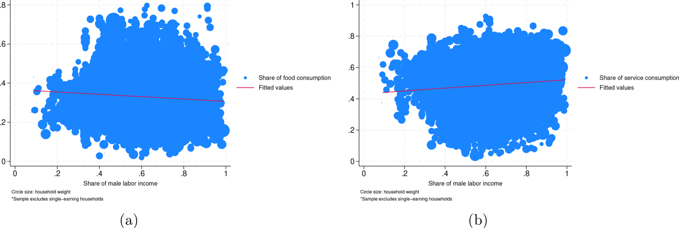
Scatter plots for level of male labor income share and consumption shares. (a) Level of male labor income share and food consumption share. (b) Level of male labor income share and service consumption share.

Income could be an endogenous outcome of intra-household bargaining, as rise in bargaining power may lead to increase in leisure and reduce relative income within the household.^[19] Hence, we additionally look at the male wage share. Figures 4 and 5 display scatter plots with a fitted line between specific consumption bundles and growth and level of male wage share, respectively. We can see similar results as when male labor income share is used as measure of bargaining power: While growth of male wage share shows weak relationships with food (panel a) and service (panel b) expenditure share, share of male wage shows a negative relationship with food expenditure share (panel a) and positive relationship with service expenditure share (panel b).

Figure 4:

Scatter plots for growth of male wage share and consumption shares. (a) Growth of male wage share and food consumption share. (b) Growth of male wage share and service consumption share.

Figure 5:

Scatter plots for level of male wage share and consumption shares. (a) Level of male wage share and food consumption share. (b) Level of male wage share and service consumption share.

Next, we compare the relationship between male housework hours share and different consumption bundle shares in terms of level. We note that households in which one of the spouses is a sole contributor in domestic chores are excluded. Panel a of Figure 6 shows the scatter and fitted line between the male housework hours and food expenditure share. We can observe a positive relationship; households with males who relatively take part in housework more than their spouses tend to consume more shares of food-related goods. An opposite relationship is depicted in panel b, where the share of male housework hours and service-related consumption share is negatively correlated.

Figure 6:

Scatter plots for level of male housework hours share and consumption shares. (a) Level of male housework hours share and food consumption share. (b) Level of male housework hours share and service consumption share.

The relationship between different proxies of bargaining power and several consumption bundle expenditure shares is shown to be uncorrelated or weakly correlated, even then in the opposite direction from what is depicted in the US data. This may be one of the driving forces of why further bias correction through controlling for additional consumption bundle shares is not clearly observed in Korean data.

4 Conclusions

Controlling for marginal utility of wealth is key in the principle of estimating the Frisch labor supply elasticity. Previous literature using Korean data attempted this through controlling for household level asset and debt, but this may still leave room for a downward bias of the estimation based on literature based on US data. Also, taking the existence of limited commitment or different bargaining positions between spouses into account seems reasonable when estimating for labor supply elasticity in Korea as noticeable differences in wage and economic participation rate between gender is observable. An improved estimation approach in which not only total household consumption is controlled but also different types of expenditure shares are additionally accounted for eliminated this bias in US data.

This analysis uses a Korean panel data from KLIPS and shows that despite different results in the magnitude of change in the estimated elasticities compared to previous literature based on US data, meaningful interpretation can be taken from the empirical results. First, a downward bias can be reduced through considering total household consumption. Second, while it is true that further bias correction through controlling for additional consumption bundle shares is not clearly observed in Korean data, with estimations increasing to only about 0.057 on average, it can be inferred that bargaining power within Korean households do not vary enough as in the US; gender rules and positions within the household may be more fixed in the case of Korea. This is partially shown in the consumption data, as there exists a weak negative to no relationship between the male share of labor income of a household and food consumption share. In other words, bargaining powers within households are not as clearly reflected in the household consumption patterns for Korean households. Hence, further research on the labor supply of South Korea considering consumption and limited commitments under households is deemed needed.

Corresponding author: Myungkyu Shim, School of Economics, Yonsei University, Seoul, South Korea, E-mail: myungkyushim@yonsei.ac.kr

We would like to thank the editor (Hendrik Schmitz) and an anonymous referee for their valuable and constructive comments. We are grateful to Youjin Hahn, Jongkwan Lee, Hee-Seung Yang, and participants at the 2024 Meeting of the Society of Economics of the Household, 16th Joint Economics Symposium of Six Leading East Asian Universities, and Yonsei Macro Reading Group for their comments. Shim gratefully acknowledges the financial support from Yonsei University and the Yongwoon Scholarship Foundation (Yonsei-Yongwoon Research Grant No. 2023-11-1234).

Funding source: Yonsei University

Award Identifier / Grant number: 2023-11-1234

Appendix A

A.1 1st Stage Regression Results for Main Analysis

The following Table A.1 shows the wage regression results for our main analysis.

Table A.1:

Wage regression results.

	Log wage rate logw _mj,t
Lagged log wage rate logw _mj,t−1	0.247^***
	(0.0076)
Log total consumption log c ̃ j , t	0.078^***
	(0.0074)
Log food share log ( c ̃ j , t , F / c ̃ j , t )	0.017^***
	(0.0061)
R ²	0.892
Number of HH	3,048
Observations	18,168

Note: Standard errors in parentheses (^*** p < 0.01, ^** p < 0.05, ^* p < 0.1). All regressions control for individual and time fixed effects, a cubic in age, and education of head (high school or less/college/grad school and up).

A.2 Original Approach of Bredemeier, Gravert and Juessen (2023) Using Log-Level Regressions

As a further robustness check, we replicate the empirical estimation equation of Bredemeier, Gravert and Juessen (2023) using the Korean data, based on public codes provided online (source: https://ideas.repec.org/c/red/ccodes/21-231.html):

(A.1) log h g j , t = η g E t log w g j , t + Γ j log C j , t + δ g j , t + χ g , t + μ g j + ϵ g j , t

where C _j,t is a vector of consumption-related variables including c ̃ j , t and c ̃ j , k , t / c ̃ j , t for all k = 1, …, K, δ _gj,t is a set of observable taste shifters such as age and number of young (age 0–6) and old (age 7–17) children, and χ _g,t and μ _gj are time and individual fixed effects, respectively.

Bredemeier, Gravert and Juessen (2023) run a first-stage wage regression on the actual wage that includes a third-order polynomial in age and interactions with education, year dummies, and other variables including taste shifters such as the number of young and old children and race. As Korea is not racially diverse, we exclude race from our regression.

The following Tables A.2 and A.3 show the regression results of the labor supply elasticity for male and female, respectively, when we incorporate the original methodology of Bredemeier, Gravert and Juessen (2023), which uses log-level data. While coefficients are smaller than what we obtained from the estimation with first-differenced data, main finding that controlling for composition of consumption items does not yield greater labor supply elasticity remains unchanged.

Table A.2:

Labor supply elasticity for men (log-level).

	(1)	(2)	(3)	(4)	(5)	(6)	(7)
Log wage rate	0.007	0.213^***	0.202^***	0.201^***	0.193^***	0.223^***	0.249^***
log w ̃ m j , t	(0.0066)	(0.0671)	(0.0690)	(0.0690)	(0.0700)	(0.0709)	(0.0705)
Log total consumption		−0.119^***	−0.113^***	−0.111^***	−0.105^***	−0.125^***	−0.133^***
log c ̃ j , t		(0.0385)	(0.0394)	(0.0390)	(0.0385)	(0.0402)	(0.0386)
Log food share			−0.002
log ( c ̃ j , t , F / c ̃ j , t )			(0.0033)
Log service share				−0.004
log ( c ̃ j , t , S / c ̃ j , t )				(0.0038)
1st principle component					−0.002	−0.005^*
					(0.0020)	(0.0027)
2nd pc	No	No	No	No	No	Yes	No
3rd pc	No	No	No	No	No	Yes	No
All consumption shares	No	No	No	No	No	No	Yes
R ²	0.549	0.549	0.549	0.549	0.549	0.549	0.550
Number of HH	3,563	3,563	3,563	3,563	3,560	3,560	3,560
Observations	22,871	22,871	22,871	22,871	22,837	22,837	22,837

Note: Dependent variable is log hours worked log h _mj,t. Standard errors in parentheses (^*** p < 0.01, ^** p < 0.05, ^* p < 0.1). All regressions control for individual and time fixed effects, a cubic in age, numbers of young (age 0–6) and old (age 7–17) children, and education of head (high school or less/college/grad school and up).

Table A.3:

Labor supply elasticity for women (log-level).

	(1)	(2)	(3)	(4)	(5)	(6)	(7)
Log wage rate	0.011	−0.075	−0.086	−0.088	−0.087	−0.079	−0.066
log w ̃ m j , t	(0.0205)	(0.0600)	(0.0645)	(0.0646)	(0.0647)	(0.0648)	(0.0654)
Log total consumption		0.036	0.039	0.042^*	0.041	0.044^*	0.043^*
log c ̃ j , t		(0.0237)	(0.0246)	(0.0248)	(0.0253)	(0.0258)	(0.0255)
Log food share			−0.004
log ( c ̃ j , t , F / c ̃ j , t )			(0.0079)
Log service share				−0.004
log ( c ̃ j , t , S / c ̃ j , t )				(0.0086)
1st principle component					−0.001	0.001
					(0.0031)	(0.0033)
2nd pc	No	No	No	No	No	Yes	No
3rd pc	No	No	No	No	No	Yes	No
All consumption shares	No	No	No	No	No	No	Yes
R ²	0.632	0.632	0.632	0.632	0.632	0.632	0.633
Number of HH	2,269	2,269	2,269	2,269	2,268	2,268	2,268
Observations	12,922	12,922	12,922	12,922	12,911	12,911	12,911

Note: Dependent variable is log hours worked log h _mj,t. Standard errors in parentheses (^*** p < 0.01, ^** p < 0.05, ^* p < 0.1). All regressions control for individual and time fixed effects, a cubic in age, numbers of young (age 0–6) and old (age 7–17) children, and education of head (high school or less/college/grad school and up).

A.3 Regression Results Additionally Controlling for Borrowing Constraints

The following Table A.4 presents the regression results of labor supply elasticity when additionally accounting for borrowing constraints, following Bredemeier, Gravert and Juessen (2019) and Kim, Shim and Yang (2022). We find that the estimated coefficients, including the interaction term between the male head’s earnings contribution and expected wage growth, are slightly higher than those in Table 3, which does not include this interaction term. This may imply that, beyond addressing limited commitment between couples, accounting for borrowing constraints may also help mitigate downward bias. However, the change in elasticity estimates between columns (2) and (3) remains subtle, similar to the main regression results in Table 3.

Table A.4:

Labor supply elasticity for men (income share).

	(1)	(2)	(3)	(4)	(5)	(6)	(7)
Log wage growth rate	0.385^***	0.454^***	0.458^***	0.460^***	0.458^***	0.450^***	0.418^***
Δ log w ̃ m j , t	(0.0830)	(0.0832)	(0.0832)	(0.0834)	(0.0835)	(0.0834)	(0.0768)
Log wage growth rate	−0.009	−0.028	−0.028	−0.030	−0.026	−0.017	0.017
X earnings contribution	(0.0981)	(0.0978)	(0.0978)	(0.0981)	(0.0982)	(0.0981)	(0.0898)
Log total consumption growth		−0.039^***	−0.042^***	−0.040^***	−0.038^***	−0.038^***	−0.038^***
Δ log c ̃ j , t		(0.0046)	(0.0048)	(0.0049)	(0.0047)	(0.0048)	(0.0051)
Log food share growth			−0.010^***
Δ log ( c ̃ j , t , F / c ̃ j , t )			(0.0038)
Log service share growth				0.002
Δ log ( c ̃ j , t , S / c ̃ j , t )				(0.0037)
1st principle component					−0.002	−0.002
					(0.0020)	(0.0022)
2nd pc	No	No	No	No	No	Yes	No
3rd pc	No	No	No	No	No	Yes	No
All consumption shares	No	No	No	No	No	No	Yes
R ²	0.109	0.114	0.115	0.114	0.115	0.115	0.115
Number of HH	2,536	2,536	2,536	2,536	2,534	2,534	2,534
Observations	14,238	14,238	14,238	14,238	14,202	14,202	14,202

Note: Dependent variable is log hours worked growth Δlogh _mj,t. Standard errors in parentheses (^*** p < 0.01, ^** p < 0.05, ^* p < 0.1). All regressions control for individual and time fixed effects, a cubic in age, range of children (0/1–2/3−) and education of head (high school or less/college/grad school and up).

References

Altonji, Joseph G. 1986. “Intertemporal Substitution in Labor Supply: Evidence from Micro Data.” Journal of Political Economy 94 (3): S176–215. https://doi.org/10.1086/261403.Search in Google Scholar

Berey, Lewis A., and Richard W. Pollay. 1968. “The Influencing Role of the Child in Family Decision Making.” Journal of Marketing Research 5 (1): 70–2. https://doi.org/10.1177/002224376800500109.Search in Google Scholar

Bittman, Michael, Paula England, Liana Sayer, Nancy Folbre, and George Matheson. 2003. “When Does Gender Trump Money? Bargaining and Time in Household Work.” American Journal of Sociology 109 (1): 186–214. https://doi.org/10.1086/378341.Search in Google Scholar

Borjas, George J. 1980. “The Relationship Between Wages and Weekly Hours of Work: The Role of Division Bias.” Journal of Human Resources 15 (3): 409–23. https://doi.org/10.2307/145291.Search in Google Scholar

Bredemeier, Christian, Jan Gravert, and Falko Juessen. 2019. “Estimating Labor Supply Elasticities with Joint Borrowing Constraints of Couples.” Journal of Labor Economics 37 (4): 1215–65. https://doi.org/10.1086/703148.Search in Google Scholar

Bredemeier, Christian, Jan Gravert, and Falko Juessen. 2023. “Accounting for Limited Commitment Between Spouses when Estimating Labor-Supply Elasticities.” Review of Economic Dynamics 51: 547–78. https://doi.org/10.1016/j.red.2023.06.002.Search in Google Scholar

Chang, Yongsung, and Sun-Bin Kim. 2006. “From Individual to Aggregate Labor Supply: A Quantitative Analysis Based on a Heterogeneous Agent Macroeconomy.” International Economic Review 47 (1): 1–27. https://doi.org/10.1111/j.1468-2354.2006.00370.x.Search in Google Scholar

Dauphin, Anyck, Abdel-Rahmen El Lahga, Bernard Fortin, and Guy Lacroix. 2011. “Are Children Decision-Makers Within the Household?” The Economic Journal 121 (553): 871–903. https://doi.org/10.1111/j.1468-0297.2010.02404.x.Search in Google Scholar

Domeij, David, and Martin Floden. 2006. “The Labor-Supply Elasticity and Borrowing Constraints: Why Estimates are Biased.” Review of Economic Dynamics 9 (2): 242–62. https://doi.org/10.1016/j.red.2005.11.001.Search in Google Scholar

Duflo, Esther. 2012. “Women Empowerment and Economic Development.” Journal of Economic Literature 50 (4): 1051–79. https://doi.org/10.1257/jel.50.4.1051.Search in Google Scholar

Geist, Claudia. 2005. “The Welfare State and the Home: Regime Differences in the Domestic Division of Labour.” European Sociological Review 21 (1): 23–41. https://doi.org/10.1093/esr/jci002.Search in Google Scholar

Hersch, Joni, and Leslie S. Stratton. 1994. “Housework, Wages, and the Division of Housework Time for Employed Spouses.” The American Economic Review 84 (2): 120–5.Search in Google Scholar

Keane, Michael P. 2011. “Labor Supply and Taxes: A Survey.” Journal of Economic Literature 49 (4): 961–1075. https://doi.org/10.1257/jel.49.4.961.Search in Google Scholar

Keane, Michael, and Richard Rogerson. 2015. “Reconciling Micro and Macro Labor Supply Elasticities: A Structural Perspective.” Annual Review of Economics 7 (1): 89–117. https://doi.org/10.1146/annurev-economics-080614-115601.Search in Google Scholar

Kim, Won Hyeok, Myungkyu Shim, and Hee-Seung Yang. 2022. “Labour Supply Elasticities in Korea: Estimation with Borrowing-Constrained Couples.” Applied Economics Letters 29 (3): 183–7. https://doi.org/10.1080/13504851.2020.1861191.Search in Google Scholar

Lundberg, Shelly J., Robert A. Pollak, and Terence J. Wales. 1997. “Do Husbands and Wives Pool Their Resources? Evidence from the United Kingdom Child Benefit.” Journal of Human Resources: 463–80. https://doi.org/10.2307/146179.Search in Google Scholar

Mazzocco, Maurizio. 2007. “Household Intertemporal Behaviour: A Collective Characterization and a Test of Commitment.” The Review of Economic Studies 74 (3): 857–95. https://doi.org/10.1111/j.1467-937x.2007.00447.x.Search in Google Scholar

Moon, Y. M. 2014. “A Panel Analysis of the Life Satisfaction of Standard and Non-Standard Workers: Focusing on Latent Growth Model.” Korean Journal of Labor Studies 20 (2): 187–218. https://doi.org/10.17005/kals.2014.20.2.187.Search in Google Scholar

Moon, Weh-Sol, and Sungju Song. 2016. “Estimating Labor Supply Elasticity in Korea.” Korean Journal of Labor Economics 39 (2): 35–51.Search in Google Scholar

Pencavel, John. 1986. “Labor Supply of Men: A Survey.” Handbook of Labor Economics 1: 3–102.10.1016/S1573-4463(86)01004-0Search in Google Scholar

Robinson, Jonathan. 2012. “Limited Insurance within the Household: Evidence from a Field Experiment in Kenya.” American Economic Journal: Applied Economics 4 (4): 140–64. https://doi.org/10.1257/app.4.4.140.Search in Google Scholar

Yang, Hyunsoo. 2021. “Gender Equality: Korea has Come a Long Way, But There is More Work to Do.” In Korea and the OECD: 25 Years and Beyond, 256–65.Search in Google Scholar

Yogev, Sara, and Jeanne Brett. 1985. “Patterns of Work and Family Involvement Among Single-and Dual-Earner Couples.” Journal of Applied Psychology 70 (4): 754. https://doi.org/10.1037//0021-9010.70.4.754.Search in Google Scholar

Received: 2024-07-23

Accepted: 2025-03-11

Published Online: 2025-03-28

This work is licensed under the Creative Commons Attribution 4.0 International License.

Articles in the same Issue

https://doi.org/10.1515/bejeap-2024-0254

Keywords for this article

Frisch labor supply elasticity; limited commitment; Korea; KLIPS

Creative Commons

BY 4.0