International Commodity-Tax Competition and Asymmetric Producer Prices

Sezer Yasar

doi:10.1515/bejeap-2022-0332

Article

International Commodity-Tax Competition and Asymmetric Producer Prices

Sezer Yasar

Published/Copyright: January 13, 2025

Published by

Become an author with De Gruyter Brill

Submit Manuscript Author Information Explore this Subject

From the journal The B.E. Journal of Economic Analysis & Policy Volume 25 Issue 1

Abstract

In this paper, I extend the seminal commodity-tax competition model of Kanbur and Keen (1993. “Jeux Sans Frontières: Tax Competition and Tax Coordination When Countries Differ in Size.” The American Economic Review 83: 877–92) letting asymmetric producer prices between countries of different sizes. Unlike Kanbur and Keen, I show that there are multiple equilibria, and at some equilibria, small-country consumers cross-shop from the large. Besides, tax harmonization can benefit the small country, and a minimum tax rate can decrease a country’s tax revenue.

Keywords: commodity-tax competition; cross-border shopping; asymmetric prices; tax harmonization; minimum tax rate

JEL Classification: H20; H77

Corresponding author: Sezer Yasar, Cardiff Business School, Cardiff University, Cardiff, CF10 3EU, UK, E-mail: yasars3@cardiff.ac.uk

Acknowledgments

I thank the participants of TED University FEAS Brown Bag Seminar, 2019 International Conference of TED University Trade Research Center, and 2019 International Conference on Public Economic Theory for stimulating discussions. I also thank editor Tobias Wenzel and two anonymous referees for their valuable comments.

A Appendix: Proof of Lemmas and Propositions

A.1 Proof of Lemma 1

A.1.1 Small Country’s Best-Response Function

Assume that T ≤ p − P − δ. Then, whatever t is all small-country consumers shop from the large country. So, we have t(T) ∈ [0, ∞).

Assume that p − P − δ < T ≤ p − P. There is no tax rate such that the large-country consumers shop from the small country. Thus, the small country’s problem is max t t h 1 − ( t + p ) − ( T + P ) δ s.t. 0 ≤ t. Solving the problem, we have t ( T ) = δ + ( T + P ) − p 2 .

Assume that p − P < T. If the small country maximizes its revenue by choosing t ≤ (T + P) − p, its problem is given as max t t h + t H ( T + P ) − ( t + p ) δ s.t. 0 ≤ t ≤ (T + P) − p. Solving the problem, we have

(5) t = ( T + P ) − p if T < δ θ + p − P , δ θ + ( T + P ) − p 2 if δ θ + p − P ≤ T .

If the small country maximizes its revenue by choosing t ≥ T + P − p, its problem is given as max t t h 1 − ( t + p ) − ( T + P ) δ s.t. T + P − p ≤ t. Solving the problem, we have

(6) t = δ + ( T + P ) − p 2 if T ≤ δ + p − P , ( T + P ) − p if δ + p − P < T .

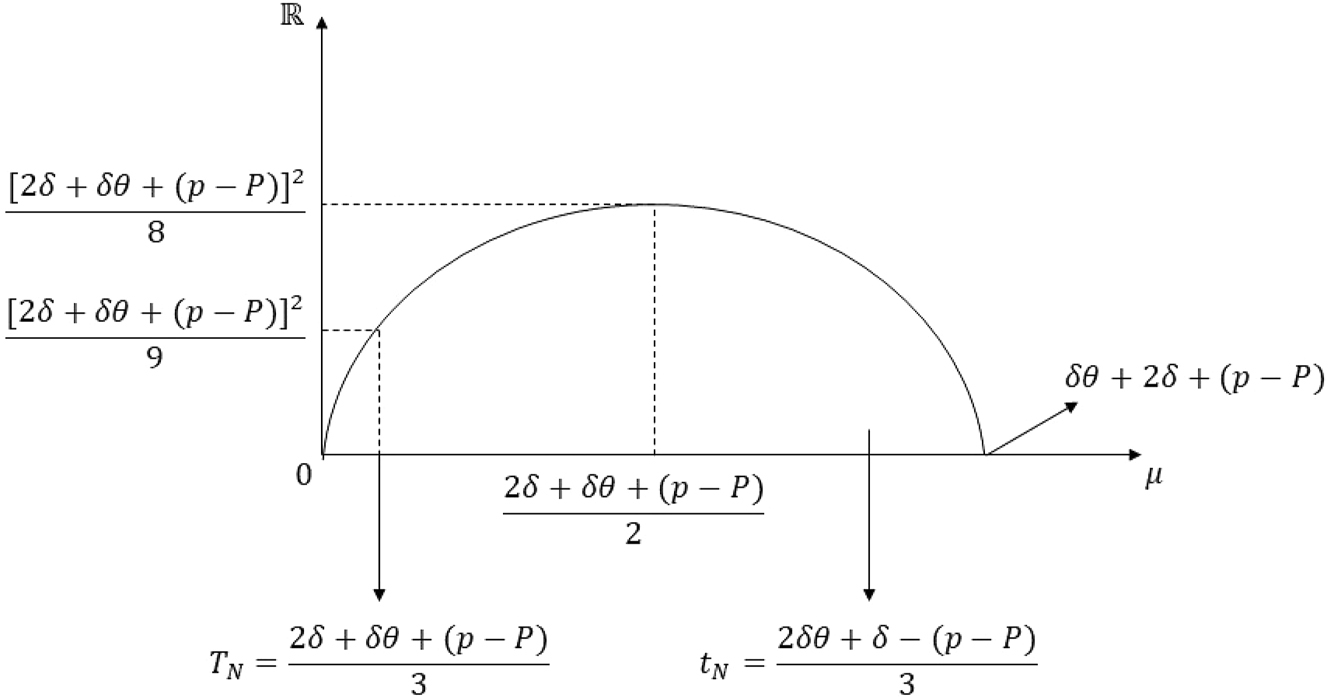
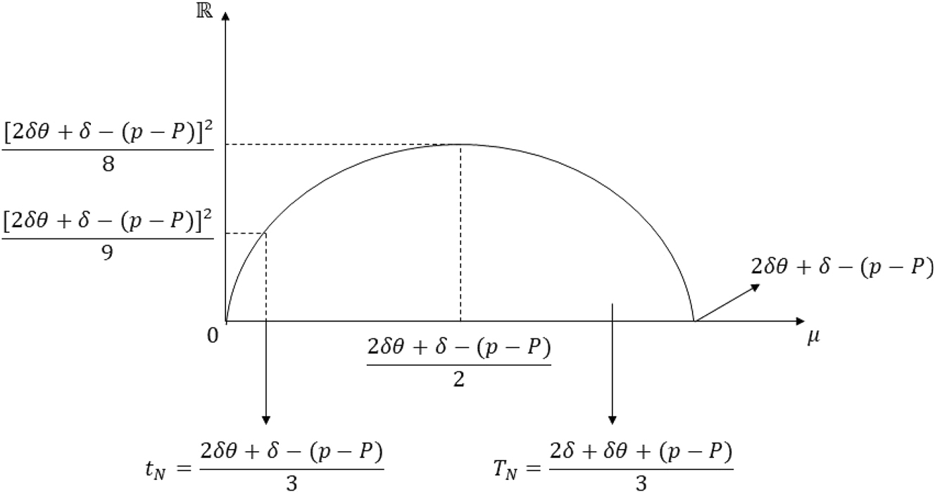
I analyze which way of maximizing its revenue is optimal for the small country under different values of θ. First, assume that θ < 1. Take T ∈ (p − P, δθ + p − P). If the small country maximizes its revenue by choosing t ≤ (T + P) − p, t = (T + P) − p by Equation (5), and its revenue is [(T + P) − p]h. If it maximizes its revenue by choosing t ≥ (T + P) − p, t = δ + ( T + P ) − p 2 by Equation (6), and its revenue is h ( δ + ( T + P ) − p ) 2 4 δ . We have h ( δ + ( T + P ) − p ) 2 4 δ > [ ( T + P ) − p ] h if and only if (δ − [(T + P) − p])² > 0 which always holds as we have δθ < δ and T < δθ + p − P. So, we have t ( T ) = δ + ( T + P ) − p 2 . Take T ∈ [δθ + p − P, δ + p − P]. If the small country maximizes its revenue by choosing t ≥ (T + P) − p, t = δ + ( T + P ) − p 2 by Equation (5), and its revenue is h ( δ + ( T + P ) − p ) 2 4 δ . If it maximizes its revenue by choosing t ≤ (T + P) − p, t = δ θ + ( T + P ) − p 2 by Equation (6), and its revenue is h ( δ θ + ( T + P ) − p ) 2 4 δ θ . We have h ( δ + ( T + P ) − p ) 2 4 δ > h ( δ θ + ( T + P ) − p ) 2 4 δ θ if and only if δ θ > ( T + P − p ) . So, we have

(7) t ( T ) = δ + ( T + P ) − p 2 if T < δ θ + p − P , δ + ( T + P ) − p 2 , δ θ + ( T + P ) − p 2 if T = δ θ + p − P .

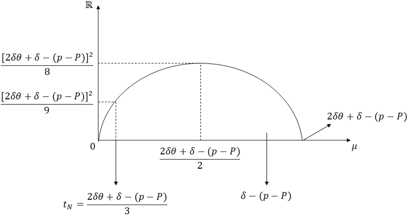
Take T > δ + p − P. If the small country maximizes its revenue by choosing t ≤ (T + P) − p, t = δ θ + ( T + P ) − p 2 by Equation (5), and its revenue is h ( δ θ + ( T + P ) − p ) 2 4 δ θ . If it maximizes its revenue by choosing t ≥ (T + P) − p, t = (T + P) − p by Equation (6), and its revenue is [(T + P) − p]h. It is easy to show that the latter revenue is higher. Thus, t ( T ) = δ θ + ( T + P ) − p 2 . Collecting the results, if θ < 1, we have

(8) t ( T ) = [ 0 . ∞ ) if T ≤ p − P − δ δ + ( T + P ) − p 2 if p − P − δ < T < δ θ + p − P , δ + ( T + P ) − p 2 , δ θ + ( T + P ) − p 2 if T = δ θ + p − P , δ θ + ( T + P ) − p 2 if δ θ + p − P < T .

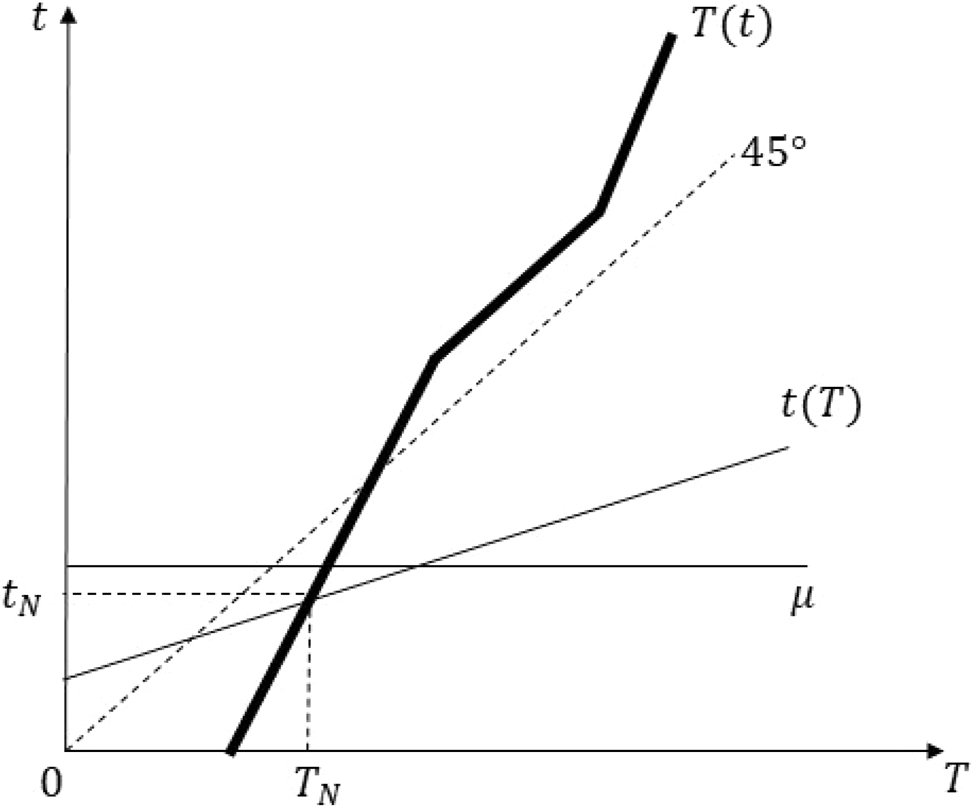
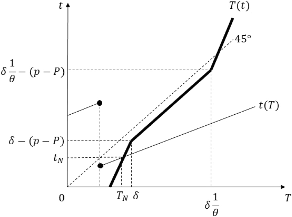
Second, assume that θ = 1. Take T ∈ (p − P, δ + p − P). If the small country maximizes its revenue by choosing t ≤ (T + P) − p, t = (T + P) − p by Equation (5), and its revenue is [(T + P) − p]h. If it maximizes its revenue by choosing t ≥ (T + P) − p, t = δ + ( T + P ) − p 2 by Equation (6), and its revenue is h ( δ + ( T + P ) − p ) 2 4 δ . We have h ( δ + ( T + P ) − p ) 2 4 δ > [ ( T + P ) − p ] h if and only if (δ − [(T + P) − p])² > 0 which always holds as we have θ = 1 and T < δθ + p − P. So, we have t ( T ) = δ + ( T + P ) − p 2 . Take T = δθ + p − P = δ + p − P. If the small country maximizes its revenue by choosing t ≤ (T + P) − p, t = δ θ + ( T + P ) − p 2 by Equation 5, and if it maximizes its revenue by choosing t ≥ (T + P) − p, t = δ + ( T + P ) − p 2 by Equation (6). Because, both tax rates are equal, as θ = 1, we have t ( T ) = δ + ( T + P ) − p 2 . Take T > δ + p − P. If the small country maximizes its revenue by choosing t ≤ (T + P) − p, t = δ θ + ( T + P ) − p 2 by Equation (5), and its revenue is h ( δ θ + ( T + P ) − p ) 2 4 δ θ . If it maximizes its revenue by choosing t ≥ (T + P) − p, t = (T + P) − p by Equation (6), and its revenue is [(T + P) − p]h. It is easy to show that the former revenue is higher. Thus, we have t ( T ) = δ + ( T + P ) − p 2 . Collecting the results, if θ = 1, we have

(9) t ( T ) = [ 0 . ∞ ) if T ≤ p − P − δ δ + ( T + P ) − p 2 otherwise .

The whole results give us the small country’s best-response function:

t ( T ) = [ 0 , ∞ ) if T ≤ p − P − δ , δ + P + T − p 2 if p − P − δ < T < δ θ + p − P , δ + P + T − p 2 , δ θ + P + T − p 2 if T = δ θ + p − P , δ θ + P + T − p 2 if δ θ + p − P < T .

A.1.2 Large Country’s Best-Response Function.

Assume that t ≤ −(p − P) − δ. Then, whatever T is all large-country consumers shop from the small country. So, we have T(t) ∈ [0, ∞).

Assume that −(p − P) − δ < t ≤ −(p − P). There is no tax rate such that the small-country consumers shop from the large country. Thus, the large country’s problem is max T T H 1 − ( T + P ) − ( t + p ) δ s.t. 0 ≤ T. Solving the problem, we have T ( t ) = δ + ( t + p ) − P 2 .

Assume that −(p − P) < t. If the large country maximizes its revenue by choosing T ≤ (t + p) − P, its problem is given as max T T H + T h ( t + p ) − ( T + P ) δ s.t. 0 ≤ T ≤ (t + p) − P. Solving the problem, we have

(10) T = ( t + p ) − P if t < δ 1 θ − ( p − P ) , δ 1 θ + ( t + p ) − P 2 if δ 1 θ − ( p − P ) ≤ t .

If the large country maximizes its revenue by choosing T ≥ t + p − P, its problem is given as max T T H 1 − ( T + P ) − ( t + p ) δ s.t. t + p − P ≤ T. Solving the problem, we have

(11) T = δ + ( t + p ) − P 2 if t ≤ δ − ( p − P ) , ( t + p ) − P if δ − ( p − P ) < t .

I analyze which way of maximizing its revenue is optimal for the small country under different values of θ.

First, assume that θ = 1. Then, clearly, the best-response function of the large country is analogous to the small country. So, we have

(12) T ( t ) = [ 0 . ∞ ) if t ≤ − ( p − P ) − δ δ + ( t + p ) − P 2 otherwise .

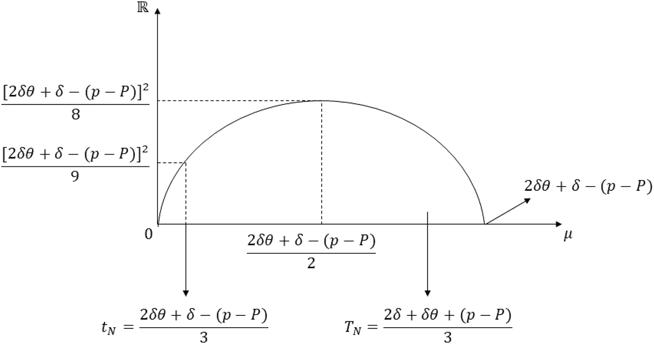
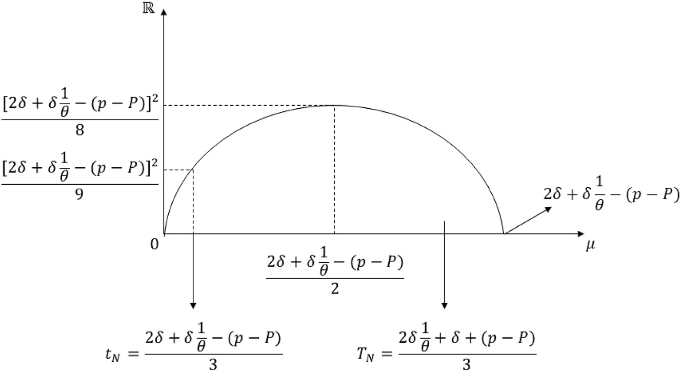
Second, assume that 1 < θ. Take t ∈ (−(p − P), δ − (p − P)). If the large country maximizes its revenue by choosing T ≤ (t + p) − P, T = (t + p) − P by Equation (10), and its revenue is [(t + p) − P]H. If it maximizes its revenue by choosing T ≥ (t + p) − P, T = δ + ( t + p ) − P 2 by Equation (11), and its revenue is H ( δ + ( t + p ) − P ) 2 4 δ . It is easy to show that the former revenue is higher. Thus, we have T ( t ) = δ + ( t + p ) − P 2 . Take t ∈ [ δ − ( p − P ) , δ 1 θ − ( p − P ) ] . Whether the large country maximizes its revenue by choosing T ≤ (t + p) − P or T ≥ (t + p) − P, it is optimal to choose T = (t + p) − P by Equations (10) and (11). So, we have T(t) = (t + p) − P. Take t > δ 1 θ − ( p − P ) . If the large country maximizes its revenue by choosing T ≤ (t + p) − P, T = δ 1 θ + ( t + p ) − P 2 by Equation (10), and its revenue is H ( δ 1 θ + ( t + p ) − P ) 2 4 δ 1 θ . If it maximizes its revenue by choosing T ≥ (t + p) − P, T = (t + p) − P by Equation (11), and its revenue is [(t + p) − P]H. It is easy to show that the latter revenue is higher if and only if t ≤ δ 1 θ − ( p − P ) . Collecting the results, we have

(13) T ( t ) = [ 0 , ∞ ) if t ≤ − ( p − P ) − δ , δ + p + t − P 2 if − ( p − P ) − δ < t ≤ δ − ( p − P ) , p + t − P if δ − ( p − P ) < t ≤ δ 1 θ − ( p − P ) , δ 1 θ + p + t − P 2 if δ 1 θ − ( p − P ) < t .

□

A.2 Proof of Proposition 1

In the following, I assume that θ ≤ 1. So, we have

t ( T ) = [ 0 , ∞ ) if T ≤ p − P − δ , δ + P + T − p 2 if p − P − δ < T < δ θ + p − P , δ + P + T − p 2 , δ θ + P + T − p 2 if T = δ θ + p − P , δ θ + P + T − p 2 if δ θ + p − P < T ,

and

(14) T ( t ) = [ 0 , ∞ ) if t ≤ − ( p − P ) − δ , δ + ( t + p ) − P 2 if − ( p − P ) − δ < t ≤ δ − ( p − P ) , ( t + p ) − P if δ − ( p − P ) < t ≤ δ 1 θ − ( p − P ) , δ 1 θ + ( t + p ) − P 2 if δ 1 θ − ( p − P ) < t .

To prove the proposition, I present both countries’ best-response correspondences and find their intersection points for each part of the proposition. Additionally, Part (iii) of the proposition is implied by Parts (ii) and (iv). Thus, I give the proof of Part (iii) after the proof of Part (iv).

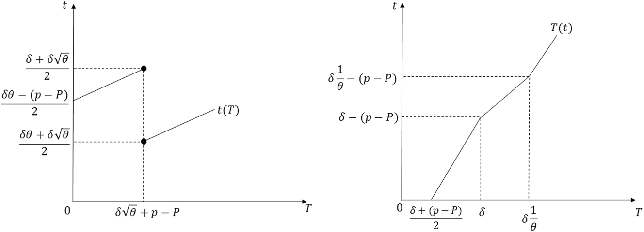
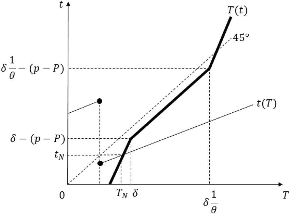
Part i: Assume that (p − P) ≤ −2δ − δθ. Then, the best-response correspondences of the small and large countries are as given in Figure 7. Under the parameter restrictions of Part (i), it is easy to show that the best-response correspondences intersect as in Figure 8. Solving for the intersection points, we get a continuum of equilibria such that T N ∈ 0 , − 2 δ − δ θ − ( p − P ) and t N = δ θ + T N − ( p − P ) 2 .

Figure 7:

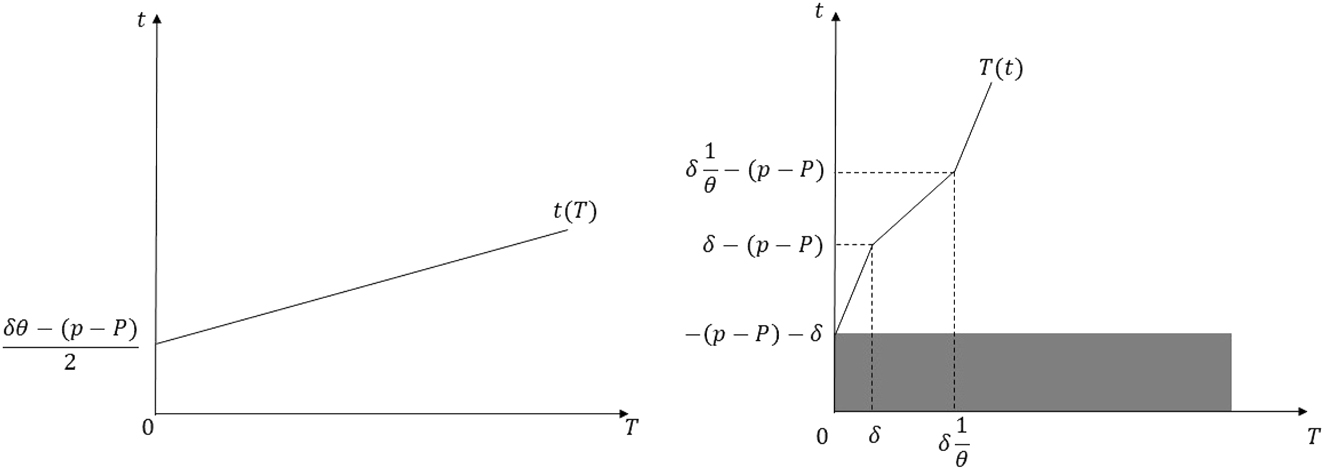
Best-response correspondences in the proof of Proposition 1 Part (i) and (ii) when −2δ − δθ < p − P ≤ −δ.

Figure 8:

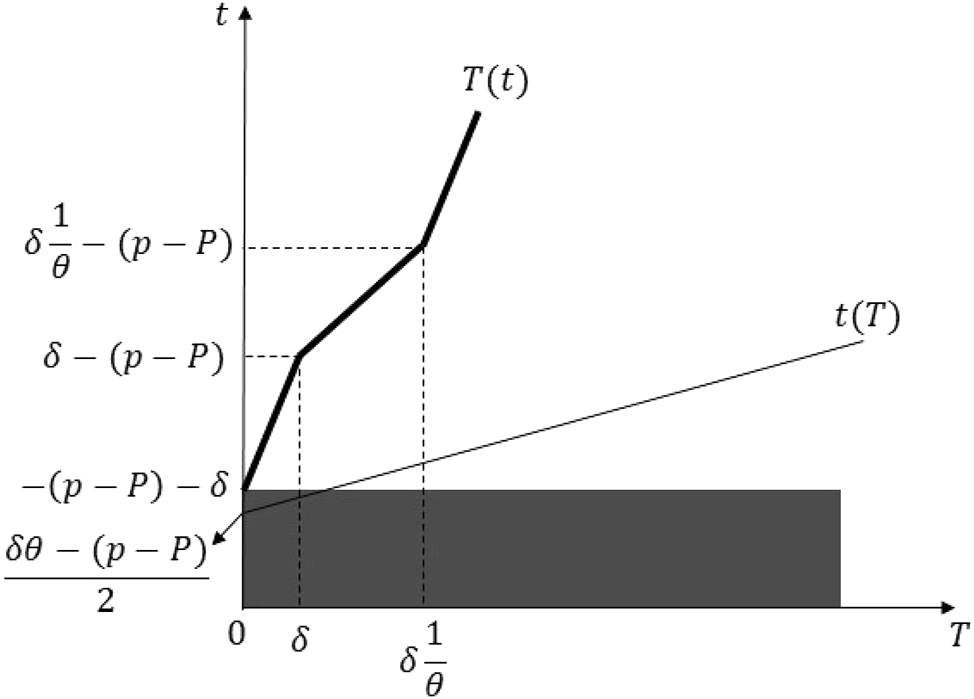
Equilibria in the proof of Proposition 1 Part (i).

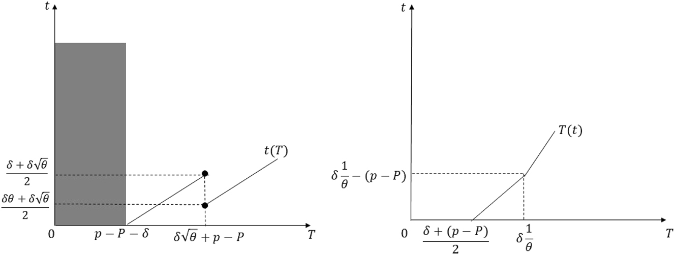
Part ii: I prove Part (ii) of the proposition under three cases, as the shape of the best-response correspondences differs. First, assume that −2δ − δθ < p − P ≤ −δ. Then, the best-response correspondences of the small and large countries are given in Figure 7. Under the parameter of our restrictions, it is easy to show that the best-response correspondences intersect as in Figure 9. Solving for the intersection points, we get the unique equilibrium ( t N , T N ) = 2 δ θ + δ − ( p − P ) 3 , 2 δ + δ θ + ( p − P ) 3 .

Figure 9:

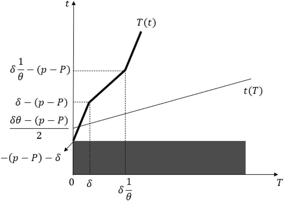
Equilibrium in the proof of Proposition 1 Part (ii) when −2δ − δθ < p − P ≤ −δ.

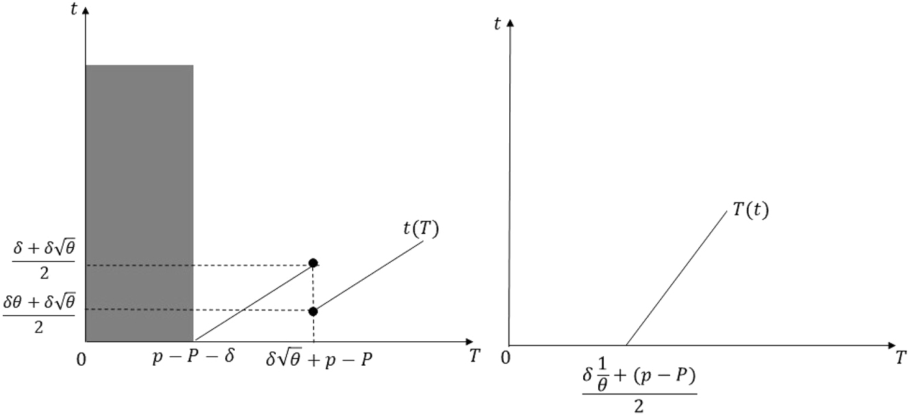
Second, assume that − δ < p − P ≤ − δ θ . Then, the best-response correspondences of the small and large countries are given in Figure 10. It is easy to show that the best-response correspondences intersect only if t ≤ δ − (p − P). For the other values of t, if solve for an intersection point, given our assumption on the parameters, the values of t or T fall out of the interval that we assume for it. If we solve for an intersection point when t ≤ δ − (p − P), we get the unique point ( t N , T N ) = 2 δ θ + δ − ( p − P ) 3 , 2 δ + δ θ + ( p − P ) 3 . We can show that, given our assumption on the parameters, t _N ≤ δ − (p − P) and T _N ≥ 0. Thus, this intersection point is the unique equilibrium.

$Figure 10: Best-response correspondences in the proof of Proposition 1 Part (ii) when − δ < p − P ≤ − δ θ $-\delta {< }p-P\le -\delta \sqrt{\theta }$ .$

Figure 10:

Best-response correspondences in the proof of Proposition 1 Part (ii) when − δ < p − P ≤ − δ θ .

Third, assume that − δ θ . < ( p − P ) ≤ δ . Then, the best-response correspondences of the small and large countries are given in Figure 11. It is easy to show that the best-response correspondences intersect only if t ≤ δ − (p − P) and δ θ + p − P ≤ T . In other cases, if we solve for an intersection point, given our assumption on the parameters, the values of t or T fall out of the interval that we assume for it. If we solve for an intersection point when t ≤ δ − (p − P) and δ θ + p − P ≤ T , we get the unique point ( t N , T N ) = 2 δ θ + δ − ( p − P ) 3 , 2 δ + δ θ + ( p − P ) 3 . We need t _N ≤ δ − (p − P) and δ θ + p − P ≤ T N which require p − P ≤ 2 δ + δ θ − 3 δ θ 2 .

$Figure 11: Best-response correspondences in the proof of Proposition 1 Part (ii) when − δ θ ≤ ( p − P ) ≤ δ $-\delta \sqrt{\theta }\le \left(p-P\right)\le \delta $ .$

Figure 11:

Best-response correspondences in the proof of Proposition 1 Part (ii) when − δ θ ≤ ( p − P ) ≤ δ .

So, collecting the results, if − δ < p − P ≤ 2 δ + δ θ − 3 δ θ 2 , we have a unique equilibrium ( t N , T N ) 2 δ θ + δ − ( p − P ) 3 , 2 δ + δ θ + ( p − P ) 3 .

Part iii. Proof Part (iii) is given after proof of Part (iv) as it is implied by the proofs of Part (ii) and (iv).

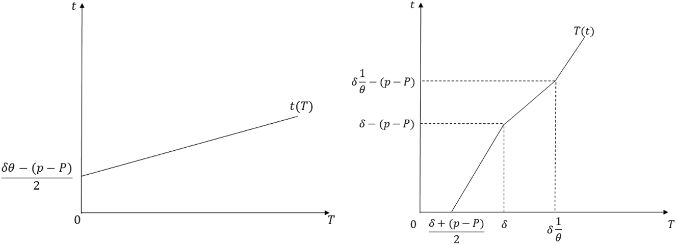
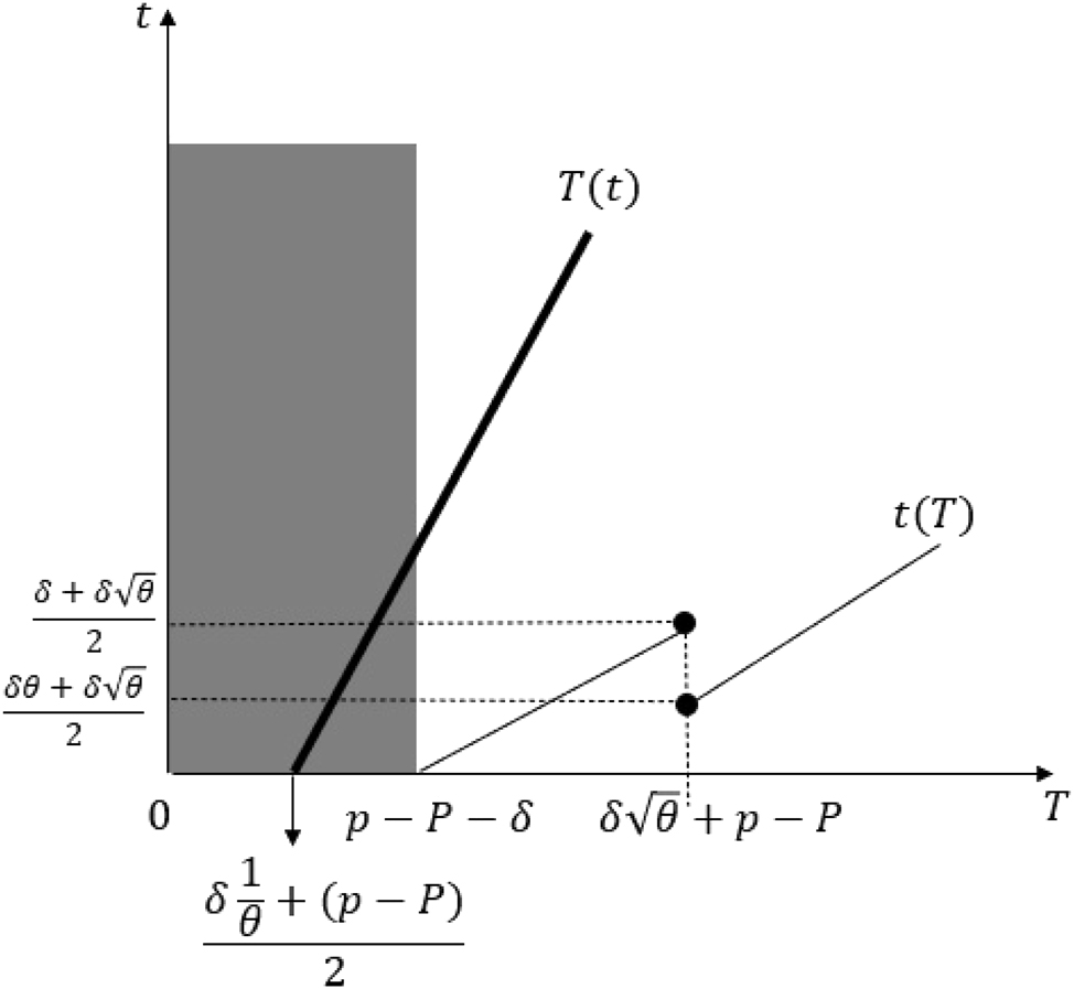
Part iv: I prove Part (iv) of the proposition under two cases, as the shape of the best-response correspondences differs under the two. First, assume that δ ≤ p − P < δ 1 θ . Then, the best-response correspondences of the small and large countries are given in Figure 12. It is easy to show that the best-response correspondences intersect only if δ 1 θ − ( p − P ) ≤ t and p − P − δ ≤ T ≤ δ θ + p − P . In other cases, if solve for an intersection point, given our assumption on the parameters, the values of t or T fall out of the interval that we assume for it. If we solve for an intersection point when δ 1 θ − ( p − P ) ≤ t and p − P − δ ≤ T ≤ δ θ + p − P , we get the unique point ( t N , T N ) = 2 δ + δ 1 θ − ( p − P ) 3 , 2 δ 1 θ + δ + p − P 3 . We need δ 1 θ − ( p − P ) ≤ t N and p − P − δ ≤ T N ≤ δ θ + p − P which require 2 δ 1 θ + δ − 3 δ θ 2 ≤ p − P .

$Figure 12: Best-response correspondences in the proof of Proposition 1 Part (iv) when δ < p − P < δ 1 θ $\delta {< }p-P{< }\delta \frac{1}{\theta }$ .$

Figure 12:

Best-response correspondences in the proof of Proposition 1 Part (iv) when δ < p − P < δ 1 θ .

Second, assume that δ 1 θ ≤ ( p − P ) ≤ δ 1 θ + 2 δ . Then, the best-response correspondences of the small and large countries are given in Figure 13. It is easy to show that the best-response correspondences intersect only if p − P − δ ≤ T ≤ δ θ + p − P . For the other ranges of T, if solve for an intersection point, given our assumption on the parameters, the values of t or T fall out of the interval that we assume for it. If we solve for an intersection point when p − P − δ ≤ T ≤ δ θ + p − P , we get the unique point ( t N , T N ) = 2 δ + δ 1 θ − ( p − P ) 3 , 2 δ 1 θ + δ + p − P 3 . We need p − P − δ ≤ T N ≤ δ θ + p − P which requires 2 δ 1 θ + δ − 3 δ θ 2 ≤ p − P .

$Figure 13: Best-response correspondences in the proof of Proposition 1 Part (iv), when δ 1 θ ≤ ( p − P ) ≤ δ 1 θ + 2 δ $\delta \frac{1}{\theta }\le \left(p-P\right)\le \delta \frac{1}{\theta }+2\delta $ , and in Part (v).$

Figure 13:

Best-response correspondences in the proof of Proposition 1 Part (iv), when δ 1 θ ≤ ( p − P ) ≤ δ 1 θ + 2 δ , and in Part (v).

Collecting the results in both parts of the proof, if max δ , 2 δ 1 θ + δ − 3 δ θ 2 ≤ p − P ≤ δ 1 θ + 2 δ , we have a unique equilibrium ( t N , T N ) = 2 δ + δ 1 θ − ( p − P ) 3 , 2 δ 1 θ + δ + p − P 3 .

Part iii. By the second part of the proof of Part (ii), there is no equilibrium if 2 δ + δ θ − 3 δ θ 2 < p − P < δ . By the proof of Part (iv), there is no equilibrium if δ < p − P < max δ , 2 δ 1 θ + δ − 3 δ θ 2 . Combining the two results, there is no equilibrium if 2 δ + δ θ − 3 δ θ 2 < p − P < max δ , 2 δ 1 θ + δ − 3 δ θ 2 .

Part v: Assume that δ 1 θ + 2 δ < p − P . Then, the best-response correspondences of the small and large countries are as given in Figure 13. Then, under the assumptions of Part (i), it is easy to show that the best-response correspondences intersect as in Figure 14. Solving for the intersection points, we get a continuum of equilibria such that t N ∈ 0 , p − P − 2 δ − δ 1 θ and T N = δ 1 θ + p − P + t N 2 . □

Figure 14:

Equilibria in the proof of Proposition 1 Part (v).

A.3 Proof of Proposition 2

We have cross-border sales from small to the large country if and only if t _N + p < T _N + P. Rewriting the condition under Type A equilibrium, by Proposition 1 Part (ii), we get p − P < δ(1 − θ). By the same proposition, we have Type A equilibrium if and only if − δ < p − P ≤ 2 δ + δ θ − 3 δ θ 2 and 2 δ + δ θ − 3 δ θ 2 < δ ( 1 − θ ) , the condition for cross-border sales from small to large country always holds.

By Proposition 1 Part (ii), we have t _N < T _N under Type A equilibrium if and only if 2 δ θ + δ − ( p − P ) 3 < 2 δ + δ θ + ( p − P ) 3 , that is − 1 2 δ ( 1 − θ ) < p − P . □

A.4 Proof of Proposition 3

We have cross-border sales from the large country to the small country if and only if T _N + P < t _N + p. Rewriting the condition using Proposition 1 Part (iv), we have δ 1 θ − 1 < p − P . We have Type B equilibrium if and only if max δ , 2 δ 1 θ + δ − 3 δ θ 2 ≤ p − P ≤ δ 1 θ + 2 δ . If max δ , 2 δ 1 θ + δ − 3 δ θ 2 = δ , we have δ 1 θ − 1 < δ ≤ p − P and so the condition for cross-border sales from the large country is satisfied. If max δ , 2 δ 1 θ + δ − 3 δ θ 2 = 2 δ 1 θ + δ − 3 δ θ 2 , we have δ 1 θ − 1 < 2 δ 1 θ + δ − 3 δ θ 2 ≤ p − P and so the condition for cross-border sales from the large country is satisfied. Thus, there are always cross-border sales from the large to the small country under a Type B equilibrium.

By Proposition 1 Part (iv), we have t _N < T _N if and only if − 1 2 δ 1 θ − 1 < p − P which always holds as under a Type B equilibrium we have 0 ≤ p − P by Proposition 1 Part (iv). □

A.5 Proof of Proposition 4

I prove the proposition under four cases depending on the parameter values.

Case 1: Assume that − 2 δ − δ θ < p − P < − 1 2 δ ( 1 − θ ) . We have cross-border sales in the small country and T _N < t _N by Proposition 2. Additionally, the tax revenues are given as R ( t N , T N ) = T N H 1 − ( P + T N ) − ( p + t N ) δ and r ( t N , T N ) = t N h + t N H ( P + T N ) − ( p + t N ) δ by Proposition 1 Part (ii) and Proposition 2. Under tax harmonization, take τ ∈ [T _N, t _N]. Then, it is easy to show that we have cross-border sales in the small country, and the tax revenues are given as R ( τ ) = τ H 1 − P − p δ and r ( τ ) = τ h + τ H P − p δ .

Part i: We have R(t _N) = R(t _N, t _N) < R(t _N, T _N) as ( P + T N ) − ( p + t N ) δ < P − p δ . Thus, considering that R(τ) is increasing, we have R(τ) < R(t _N, T _N) for all τ ∈ [T _N, t _N].

Part ii: We have r(t _N, T _N) < r(t _N) as ( P + T N ) − ( p + t N ) δ < P − p δ . We also have r(T _N) = r(T _N, T _N) < r(t _N, T _N). Thus, considering that r(τ) is increasing, there exits τ ̄ such that r(t _N, T _N) < r(τ) if and only if τ ̄ < τ .

Case 2: Assume that − 1 2 δ ( 1 − θ ) < p − P < 0 . We have cross-border sales in the small country and t _N < T _N by Proposition 2. Additionally, the tax revenues are given as R ( t N , T N ) = T N H 1 − ( P + T N ) − ( p + t N ) δ and r ( t N , T N ) = t N h + t N H ( P + T N ) − ( p + t N ) δ by Proposition 1 Part (ii) and Proposition 2. Under tax harmonization, take τ ∈ [t _N, T _N]. Then, it is easy to show that we have cross-border sales in small the country, and the tax revenues are given as R ( τ ) = τ H 1 − P − p δ and r ( τ ) = τ h + τ H P − p δ .

Part i: We have r(T _N) = r(T _N, T _N) < r(t _N, T _N) as P − p δ < ( P + T N ) − ( p + t N ) δ . We also have r(T _N) = r(T _N, T _N) < r(t _N, T _N). Thus, considering that r is increasing, r(τ) < r(t _N, T _N) for all τ ∈ [t _N, T _N].

Part ii: We have R(T _N) > R(t _N, T _N) as P − p δ < ( P + T N ) − ( p + t N ) δ . We also have R(t _N) = R(t _N, t _N) < R(t _N, T _N). Thus, considering that R is increasing, there exists τ ̄ ∈ [ t N , T N ] such that R(t _N, T _N) < R(τ) if and only if τ ̄ < τ .

Case 3: Assume that 0 < p − P ≤ 2 δ + δ θ − 3 δ θ 2 . We have cross-border sales in the small country and t _N < T _N by Proposition 2. Additionally, the tax revenues are given as R ( t N , T N ) = T N H 1 − ( P + T N ) − ( p + t N ) δ and r ( t N , T N ) = t N h + t N H ( P + T N ) − ( p + t N ) δ by Proposition 1 Part (ii) and Proposition 2. Under tax harmonization, take τ ∈ [t _N, T _N]. Then, it is easy to show that we have cross-border sales in the large country, and the tax revenues are given as R ( τ ) = τ H + τ h p − P δ and r ( τ ) = τ h 1 − p − P δ .

Part i: We have r(T _N) = r(T _N, T _N) < r(t _N, T _N). Thus, considering that r is increasing, r(τ) < r(t _N, T _N) for all τ ∈ [t _N, T _N].

Part ii: We have R(T _N) > R(t _N, T _N) as p − P δ > p + t N − ( P + T N ) δ . We also have R(t _N) = R(t _N, t _N) < R(t _N, T _N). Thus, considering that R is increasing, there exists τ ̄ ∈ [ t N , T N ] such that R(t _N, T _N) < R(τ) if and only if τ ̄ < τ .

Case 4: Assume that max δ , 2 δ 1 θ + δ − 3 δ θ 2 ≤ p − P ≤ δ 1 θ + 2 δ . We have cross-border sales in the large country and t _N < T _N by Proposition 3. We have r(T _N) = r(T _N, T _N) < r(t _N, T _N). Additionally, the tax revenues are given as R ( t N , T N ) = T N H + T N h p + t N − ( P + T N ) δ and r ( t N , T N ) = t N h 1 − p + t N − ( P + T N ) δ by Proposition 1 Part (iv) and Proposition 3. Under tax harmonization, take τ ∈ [t _N, T _N]. Then, it is easy to show that we have cross-border sales in the large country, and R ( τ ) = τ H + τ h p − P δ and r ( τ ) = τ h 1 − p − P δ .

Part i: We have r(T _N) = r(T _N, T _N) < r(t _N, T _N). Thus, considering that r is increasing, r(τ) < r(t _N, T _N) for all τ ∈ [t _N, T _N].

A.6 Proof of Proposition 5

Under a minimum-tax rate, I show the equilibrium tax rates by t _m and T _m for the small and large countries, respectively.

Part i: Assume that − δ θ < p − P < 2 δ + δ θ − 3 δ θ 2 . Then, we have t N = 2 δ θ + δ − ( p − P ) 3 < 2 δ + δ θ + ( p − P ) 3 = T N by Proposition 1 Part (ii), and cross-shopping in the small country by Proposition 2. These imply that we have R ( t N , T N ) = H 1 δ δ θ + 2 δ + p − P 3 2 and r ( t N , T N ) = H 1 δ 2 δ θ + δ − ( p − P ) 3 2 . Assume further that 1 4 δ ( 1 − θ ) < p − P < 2 δ + δ θ − 3 δ θ 2 . so that we have δ − ( p − P ) < T N < δ 1 θ − ( p − P ) . Then, the equilibrium is as given in Figure 15.

Figure 15:

Equilibrium in the proof of Proposition 5 Part (i).

Take the minimum tax rate μ ∈ δ − ( p − P ) , T N . Then, we have t _m = μ < μ + p − P = T _m. There are cross-border sales if and only if μ + t _m ≠ T _m + P, that is, μ ≠ μ which never holds. So, there is no cross-border sale under the minimum tax rate.

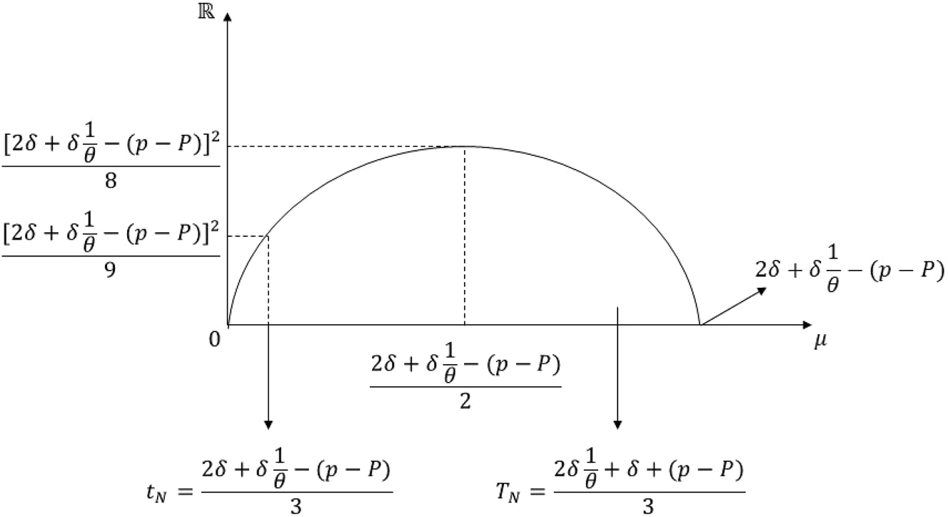
We have R(μ) = (μ + p − P)H. Then R(μ) > R(t _N, T _N) if and only if ( μ + p − P ) H > T H 1 − T + P − ( t + p ) δ , that is, δ ( μ + p − P ) > δ θ + 2 δ + p − P 3 2 . For the minimum value of μ, the left-hand side of this inequality is δ ². Additionally, we have δ 2 > δ θ + 2 δ + p − P 3 2 if and only if p − P < δ(1 − θ) which always holds as 2 δ + δ θ − 3 δ θ 3 < δ ( 1 − θ ) .

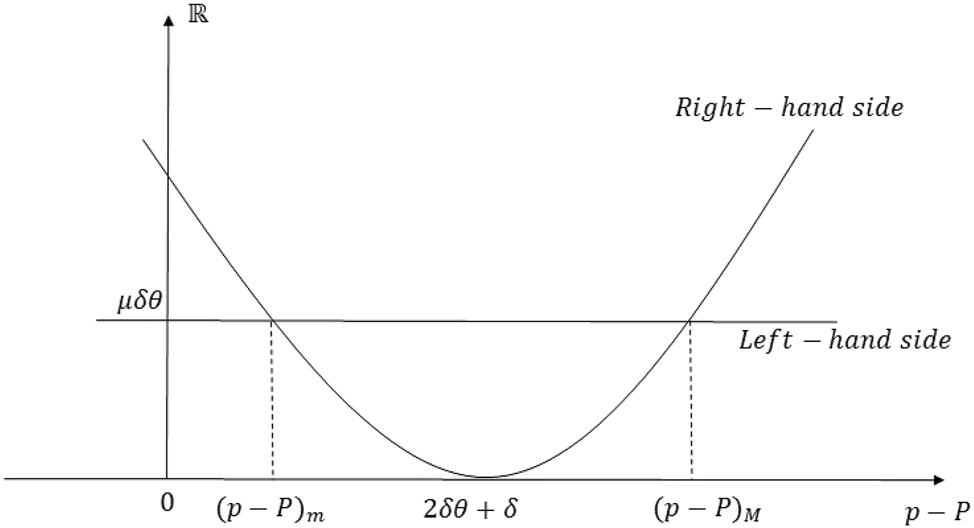
We have r(μ) = μh. Then, r(μ) > r(t _N, T _N) if and only if μ h > H 1 δ 2 δ θ + δ − ( p − P ) 3 2 , that is, μ δ θ > 2 δ θ + δ − ( p − P ) 3 2 . It is easy to show that the graph of both sides of this inequality is as given in Figure 16. So, there exists (p − P)_m and (p − P)_M such that a minimum tax rate increases the small country’s tax revenue if and only if (p − P)_m < p − P < (p − P)_M.

Figure 16:

Graph of the inequality in the proof of Proposition 5 Part (i).

Part ii: I prove Part (ii) of the proposition by considering different cases for the value of p − P, as the figure of the best-response correspondences and the range of the feasible values of the minimum-tax rate differ under each case.

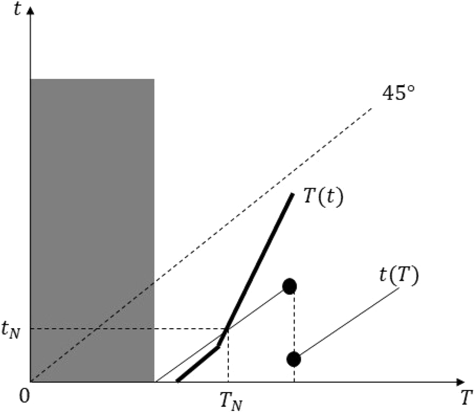
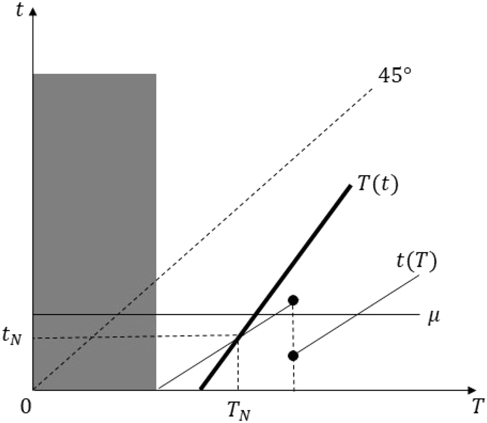
Case 1: Assume that −2δ − δθ < p − P ≤ δ. Then, under a minimum tax rate μ ∈ [T _n, t _n], the best-response correspondences are given in Figure 17. As shown by the dashed lines and the lightly shadowed area, both countries’ best-response correspondences are irrelevant for the other country’s tax rate below μ. Then, as seen in the graph, the best-response correspondences do not intersect and we do not have an equilibrium. So, I continue to the proof, by focusing on the remaining cases.

Figure 17:

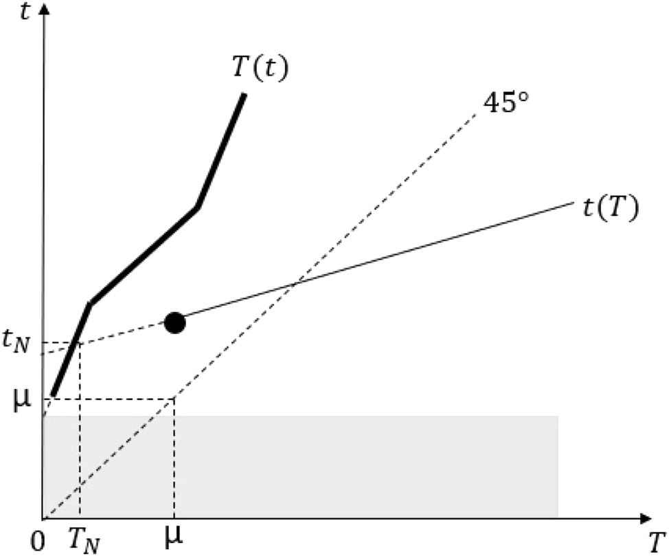
Best-response correspondences in Case 1 of proof of Proposition 5 Part (ii).

Case 2: Assume that − δ < p − P < min − δ θ , − 1 2 δ ( 1 − θ ) . Then, we have T N = 2 δ + δ θ + ( p − P ) 3 < 2 δ θ + δ − ( p − P ) 3 = t N by Proposition 1 Part (ii), and cross-shopping in the small country by Proposition 2. These imply that we have R ( t N , T N ) = H 1 δ δ θ + 2 δ + p − P 3 2 and r ( t N , T N ) = H 1 δ 2 δ θ + δ − ( p − P ) 3 2 and the equilibrium is as given in Figure 18.

Figure 18:

Equilibrium in Case 2 of proof of Proposition 5 Part (ii).

Following the discussion in Section 4, under a minimum-tax rate μ ∈ [T _N, t _N], we can ignore T(t) for t < μ. Additionally, as T can not be less than μ, for values of t > μ, we have T = μ until the value of t is such that T(t) = μ. And t(T) will get longer before the discontinuity point and will be equal to μ before the value of T is such that t(T) = μ. Then, we have T m = μ < δ θ + μ − ( p − P ) 2 = t m . Under the minimum tax rate, there are cross-border sales in the small country if and only if t _m + p < T _m + P, that is, δθ + (p − P) < μ which always holds as μ ≥ T _N.

We have R ( μ ) = T m H 1 − T m + P − ( t m + p ) δ = μ H 2 δ − μ + ( p − P ) + δ θ 2 δ . Notice that R(μ) > R(t _N, T _N) if and only if δ θ + 2 δ + ( p − P ) μ − μ 2 2 > δ θ + 2 δ + p − P 2 9 . It is easy to show that the graph of the left-hand side of this inequality is as given in Figure 19. Then, the minimum tax rate increases the large country’s tax revenue if and only if δ θ + 2 δ + ( p − P ) 3 < μ < δ θ + 2 δ + ( p − P ) 2 + δ θ + 2 δ + ( p − P ) 2 − δ θ + 2 δ + ( p − P ) 3 , that is, δ θ + 2 δ + ( p − P ) 3 < μ < 2 [ δ θ + 2 δ + ( p − P ) ] 3 which always holds as T N < μ < t N < 2 [ δ θ + 2 δ + ( p − P ) ] 3 .

Figure 19:

Graph of the inequality in Case 1 of proof of Proposition 5 Part (ii).

We have r ( μ ) = t m h + t m H T m + P − ( t m + p ) δ = 1 δ H δ θ + μ − ( p − P ) 2 2 . Then, r(μ) > r(t _N, T _N) if and only if μ > δ θ + 2 δ + ( p − P ) 3 which always holds as μ > T _N.

So, for Case 2, we have μ ̄ = t N .

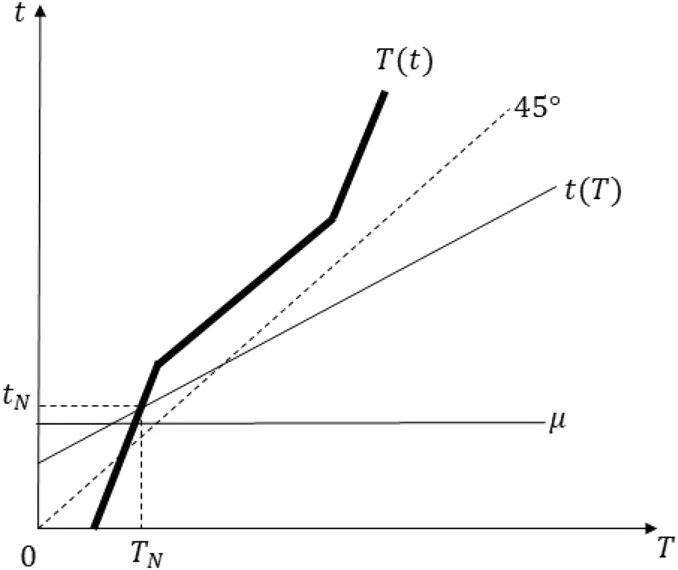
Case 3: Assume that − 1 2 δ ( 1 − θ ) < p − P < − δ θ . Then, we have t N = 2 δ θ + δ − ( p − P ) 3 < 2 δ + δ θ + ( p − P ) 3 = T N by Proposition 1 Part (ii), and cross-shopping in the small country by Proposition 2. These imply that we have R ( t N , T N ) = H 1 δ δ θ + 2 δ + p − P 3 2 and r ( t N , T N ) = H 1 δ 2 δ θ + δ − ( p − P ) 3 2 and the equilibrium is as given in Figure 20.

Figure 20:

Equilibrium Case 3 of proof of Proposition 5 Part (ii).

Following the discussion in Section 4, under a minimum-tax rate μ ∈ [t _N, T _N], we can ignore T(t) for t < μ. And t(T) will get longer before the discontinuity point and will be equal to μ before the value of T such that t(T) = μ. Then, we have t m = μ < δ + μ + ( p − P ) 2 = T m . There are cross-border sales in the small country if and only if t _m + p < T _m + P, that is, p − P < δ − μ. Notice that we have δ − T _N < δ − μ < δ − t _N, that is, δ − 2 δ + δ θ + ( p − P ) 3 < δ − μ < δ − 2 δ θ + δ + ( p − P ) 3 . By the left-hand side of this inequality, we have δ − δ θ − ( p − P ) 3 < δ − μ . Assume that we have δ − δ θ − ( p − P ) 3 < p − P . This implies that 1 4 δ ( 1 − θ ) < p − P which contradicts our assumption for Case 3. So, there are always cross-border sales in the small country.

We have R ( μ ) = T m H 1 − T m + P − ( t m + p ) δ = H 1 δ μ + δ + ( p − P ) 2 2 . Notice that R(μ) > R(t _N, T _N) if and only if H 1 δ μ + δ + ( p − P ) 2 2 > H 1 δ δ θ + 2 δ + p − P 3 2 , that is, μ > 2 δ θ + δ − ( p − P ) 3 = t N which always holds as μ > t _N.

We have r ( μ ) = t m h + t m H T m + P − ( t m + p ) δ = H 1 δ − μ 2 + 2 δ θ + δ − ( p − P μ 2 . Then, r(μ) > r(t _N, T _N) if and only if − μ 2 + 2 δ θ + δ − ( p − P μ 2 > 2 δ θ + δ − ( p − P ) 3 2 . It is easy to show that the graph of the left-hand side of the above inequality is given in Figure 21. Then, the minimum tax rate increases the small country’s tax revenue if and only if 2 δ θ + δ − ( p − P ) 3 < μ < 2 δ θ + δ − ( p − P ) 2 + 2 δ θ + δ − ( p − P ) 2 − 2 δ θ + δ − ( p − P ) 3 that is 2 δ θ + δ − ( p − P ) 3 < μ < 2 [ 2 δ θ + δ − ( p − P ) ] 3 which always holds as t N < μ < T N < 2 [ 2 δ θ + δ − ( p − P ) ] 3 .

Figure 21:

Graph of the inequality in Case 3 of proof of Proposition 5 Part (ii).

So, for Case 3, we have μ ̄ = T N .

Case 4: Assume that − δ θ < p − P < 2 δ + δ θ − 3 δ θ 2 . Then, we have t N = 2 δ θ + δ − ( p − P ) 3 < 2 δ + δ θ + ( p − P ) 3 = T N by Proposition 1 Part (ii), and cross-shopping in the small country by Proposition 2. These imply that we have R ( t N , T N ) = H 1 δ δ θ + 2 δ + p − P 3 2 and r ( t N , T N ) = H 1 δ 2 δ θ + δ − ( p − P ) 3 2 , and the equilibrium given in Figure 22.

Figure 22:

Equilibrium in Case 3 of proof of Proposition 5 Part (ii).

Case 4.i: Assume that − δ θ < p − P < 1 4 δ ( 1 − θ ) so that we have T _N < δ − (p − P). Take the minimum tax rate μ ∈ t N , T N . Then, we have t m = μ < δ + μ + ( p − P ) 2 = T m . We have cross-border sales in the small country if and only if t _m + p < T _m + P, that is, μ < δ − (p − P) which always holds as μ < T _N < δ − (p − P). So, there are always cross-border sales in the small country.

We have r ( μ ) = t m h + t m H T m + P − ( t m + p ) δ = H 1 δ − μ 2 + 2 δ θ + δ − ( p − P μ 2 . Then r(μ) > r(t _N, T _N) if and only if H 1 δ − μ 2 + 2 δ θ + δ − ( p − P μ 2 > H 1 δ 2 δ θ + δ − ( p − P ) 3 2 , that is, − μ 2 + 2 δ θ + δ − ( p − P μ 2 > 2 δ θ + δ − ( p − P ) 3 2 . It is easy to show that the graph of the left-hand side of this inequality is given in Figure 23. Then, the minimum tax rate increases the small country’s tax revenue if and only if 2 δ θ + δ − ( p − P ) 3 < μ < 2 δ θ + δ − ( p − P ) 2 + 2 δ θ + δ − ( p − P ) 2 − 2 δ θ + δ − ( p − P ) 3 , that is, 2 δ θ + δ − ( p − P ) 3 < μ < 2 [ 2 δ θ + δ − ( p − P ) ] 3 .

Figure 23:

Graph of the inequality in Case 4(i) of the proof of Proposition 5 Part (ii).

So, for Case 4.i, we have μ ̄ = 2 [ 2 δ θ + δ − ( p − P ) ] 3 .

Case 4.ii: Assume that 1 4 δ ( 1 − θ ) < p − P < 2 δ + δ θ − 3 δ θ 2 . so that we have δ − ( p − P ) < T N < δ 1 θ − ( p − P ) . Take the minimum tax rate μ ∈ t N , δ − ( p − P ) . Then, we have t m = μ < δ + μ + ( p − P ) 2 = T m . There is still a cross-border sale in the small country if and only if t _m + p < T _m + P, that is, p − P < δ − μ. Notice that by our assumption about the parameters, in this case, we have δ − ( δ − ( p − P ) ) < δ − μ < δ − 2 δ θ + δ + ( p − P ) 3 , that is, p − P < δ − μ < 2 δ − 2 δ θ + p − P 3 . So, we always have a cross-border sale in the small country.

We have r ( μ ) = t m h + t m H T m + P − ( t m + p ) δ = H 1 δ − μ 2 + 2 δ θ + δ − ( p − P μ 2 . Then, r(μ) > r(t _N, T _N) if and only if H 1 δ − μ 2 + 2 δ θ + δ − ( p − P μ 2 > H 1 δ 2 δ θ + δ − ( p − P ) 3 2 , that is, − μ 2 + 2 δ θ + δ − ( p − P μ 2 > 2 δ θ + δ − ( p − P ) 3 2 . It is easy to show that the graph of the left-hand side of this inequality is given in Figure 24. Then, the minimum tax rate increases the small country’s tax revenue if and only if 2 δ θ + δ − ( p − P ) 3 < μ < 2 δ θ + δ − ( p − P ) 2 + 2 δ θ + δ − ( p − P ) 2 − 2 δ θ + δ − ( p − P ) 3 , that is, 2 δ θ + δ − ( p − P ) 3 < μ < 2 [ 2 δ θ + δ − ( p − P ) ] 3 .

Figure 24:

Graph of the inequality in Case 4(ii) of proof of Proposition 5 Part (ii).

So, for Case 4.ii, we have μ ̄ = 2 [ 2 δ θ + δ − ( p − P ) ] 3 .

Case 5: Assume that max δ , 2 δ 1 θ + δ − 3 δ θ 2 < p − P < δ 1 θ . Then, we have t N = 2 δ + δ 1 θ − ( p − P ) 3 < T N = 2 δ 1 θ + δ + p − P 3 by Proposition 1 Part (iv), and cross-shopping in the large country by Proposition 2. These imply that we have R ( t N , T N ) = h 1 δ 2 δ 1 θ + δ + p − P 3 2 and r ( t N , T N ) = h 1 δ 2 δ + δ 1 θ − ( p − P ) 3 2 and the equilibrium given in Figure 25. Following the discussion in Section 4, under a minimum-tax rate μ ∈ [t _N, T _N], we can ignore T(t) for t < μ. And t(T) will be equal to μ before the μ-line cuts t(T) in its middle part, get longer before the discontinuity point, and will be equal to μ before the value of T is such that t(T) = μ. Then, we have t m = μ < δ 1 θ + μ + ( p − P ) 2 = T m . There is a cross-border sale in the large country if and only if T _m + P < t _m + p, that is, δ 1 θ − ( p − P ) < μ . Assume that μ < δ 1 θ − ( p − P ) so that there is a cross-border sale in the small country. For this to hold, we need t N < δ 1 θ − ( p − P ) which implies that p − P < δ 1 θ − δ . For this to hold, we need 2 δ 1 θ + δ − 3 δ θ 2 < δ 1 θ − δ , that is, 1 < θ which never holds. So, there is always cross-border sale in the large country.

Figure 25:

Equilibrium in Case 5 of proof of Proposition 5 Part (ii).

We have R ( μ ) = T m H + T m h t m + p − ( T m + P ) δ = h 1 δ δ 1 θ + μ + ( p − P ) 2 2 . Then, R(μ) ≥ R(t _N, T _N) if and only if h 1 δ δ 1 θ + μ + ( p − P ) 2 2 ≥ h 1 δ 2 δ 1 θ + δ + p − P 3 2 , that is, μ ≥ δ 1 θ + 2 δ − ( p − P ) 3 = T N which always holds as μ > T _N.

We have r ( μ ) = t m h 1 − t m + p − ( T m + P ) δ = h 1 δ μ 2 δ − μ + δ 1 θ − ( p − P ) 2 . Then, r ( μ ) ≥ r ( t N , T ) N if and only if h 1 δ μ 2 δ − μ + δ 1 θ − ( p − P ) 2 > h 1 δ 2 δ + δ 1 θ − ( p − P ) 3 2 , that is, μ 2 δ − μ + δ 1 θ − ( p − P ) 2 > 2 δ + δ 1 θ − ( p − P ) 3 2 . It is easy to show that the graph of the left-hand side of this inequality is given in Figure 26. Then, the minimum tax rate increases the small country’s tax revenue if and only if 2 δ + δ 1 θ − ( p − P ) 3 < μ < 2 δ + δ 1 θ − ( p − P ) 2 + 2 δ + δ 1 θ − ( p − P ) 2 − 2 δ + δ 1 θ − ( p − P ) 3 , that is, 2 δ + δ 1 θ − ( p − P ) 3 < μ < 2 [ 2 δ + δ 1 θ − ( p − P ) ] 3 .

Figure 26:

Graph of the inequality in the proof of Case 5 of proof of Proposition 5 Part (ii).

So, for Case 5, we have μ ̄ = 2 [ 2 δ + δ 1 θ − ( p − P ) ] 3 .

Case 6: Assume that δ 1 θ < p − P < δ 1 θ + 2 δ . Then, we have t N = 2 δ + δ 1 θ − ( p − P ) 3 < T N = 2 δ 1 θ + δ + p − P 3 by Proposition 1 Part (iv), and cross-shopping in the large country by Proposition 2. These imply that we have R ( t N , T N ) = h 1 δ 2 δ 1 θ + δ + p − P 3 2 and r ( t N , T N ) = h 1 δ 2 δ + δ 1 θ − ( p − P ) 3 2 and the equilibrium is as given in Figure 27.

Figure 27:

Equilibrium in Case 6 of the proof of Proposition 5 Part (ii).

Following the discussion in Section 4, under a minimum-tax rate μ ∈ [t _N, T _N], we can ignore T(t) for t < μ. And t(T) will be equal to μ before μ-line cuts t(T) in its middle part, get longer before the discontinuity point, and will be equal to μ before the value of T is such that t(T) = μ. Then we have t m = μ < δ 1 θ + μ + ( p − P ) 2 = T m . There is a cross-border sale in the large country if and only if T _m P < t _n + p, that is, δ 1 θ − ( p − P ) < μ which always holds as δ 1 θ − ( p − P ) < 0 < t N < μ .

We have R ( μ ) = T m H + T m h t m + p − ( T m + P ) δ = h 1 δ δ 1 θ + μ + ( p − P ) 2 2 . Then, R(μ) ≥ R(t _N, T _N) if and only if h 1 δ δ 1 θ + μ + ( p − P ) 2 2 ≥ h 1 δ 2 δ 1 θ + δ + p − P 3 2 , that is, μ ≥ δ 1 θ + 2 δ − ( p − P ) 3 = t N which always holds as μ > t _N.

We have r ( μ ) = t m h 1 − t m + p − ( T m + P ) δ = h 1 δ μ 2 δ − μ + δ 1 θ − ( p − P ) 2 . Then, r(μ) ≥ r(t _N, T _N) if and only if h 1 δ μ 2 δ − μ + δ 1 θ − ( p − P ) 2 > h 1 δ 2 δ + δ 1 θ − ( p − P ) 3 2 , that is, μ 2 δ − μ + δ 1 θ − ( p − P ) 2 > 2 δ + δ 1 θ − ( p − P ) 3 2 . It is easy to show that the graph of the left-hand side of the above inequality is as given in Figure 28. Then, the minimum tax rate increases the small country’s tax revenue if and only if 2 δ + δ 1 θ − ( p − P ) 3 < μ < 2 δ + δ 1 θ − ( p − P ) 2 + 2 δ + δ 1 θ − ( p − P ) 2 − 2 δ + δ 1 θ − ( p − P ) 3 , that is, 2 δ + δ 1 θ − ( p − P ) 3 < μ < 2 [ 2 δ + δ 1 θ − ( p − P ) ] 3 .

Figure 28:

Graph of the inequality in Case 6 of proof of Proposition 5 Part (ii).

So, for Case 6, we have μ ̄ = 2 [ 2 δ + δ 1 θ − ( p − P ) ] 3 . □

References

Agrawal, D. R. 2012. “Games within Borders: Are Geographically Differentiated Taxes Optimal?” International Tax and Public Finance 19: 574–97. https://doi.org/10.1007/s10797-012-9235-y.Search in Google Scholar

Asplund, M., R. Friberg, and F. Wilander. 2007. “Demand and Distance: Evidence on Cross-Border Shopping.” Journal of Public Economics 91: 141–57, https://doi.org/10.1016/j.jpubeco.2006.05.006.Search in Google Scholar

Behrens, K., J. H. Hamilton, G. I. Ottaviano, and J. F. Thisse. 2009. “Commodity Tax Competition and Industry Location under the Destination and the Origin Principle.” Regional Science and Urban Economics 39: 422–33. https://doi.org/10.1016/j.regsciurbeco.2009.01.008.Search in Google Scholar

Cai, H., and D. Treisman. 2005. “Does Competition for Capital Discipline Governments? Decentralization, Globalization, and Public Policy.” The American Economic Review 95: 817–30. https://doi.org/10.1257/0002828054201314.Search in Google Scholar

Cnossen, S. 2003. “How Much Tax Coordination in the European Union?” International Tax and Public Finance 10: 625–49. https://doi.org/10.1023/a:1026373703108.10.1023/A:1026373703108Search in Google Scholar

Cremer, H., and F. Gahvari. 2006. “Which Border Taxes? Origin and Destination Regimes with Fiscal Competition in Output and Emission Taxes.” Journal of Public Economics 90: 2121–42, https://doi.org/10.1016/j.jpubeco.2005.08.011.Search in Google Scholar

Devereux, M. P., B. Lockwood, and M. Redoano. 2007. “Horizontal and Vertical Indirect Tax Competition: Theory and Some Evidence from the USA.” Journal of Public Economics 91: 451–79. https://doi.org/10.1016/j.jpubeco.2006.07.005.Search in Google Scholar

DHA. 2022. Bulgarlar alisveris icin Edirne’ye akin etti. Birgun. https://www.birgun.net/haber/bulgarlar-alisveris-icin-edirne-ye-akin-etti-bin-leva-bozdurdum-ve-10-bin-lira-harcadim-400566.Search in Google Scholar

Di Matteo, L., and R. Di Matteo. 1996. “An Analysis of Canadian Cross-Border Travel.” Annals of Tourism Research 23: 103–22. https://doi.org/10.1016/0160-7383(95)00038-0.Search in Google Scholar

Eichner, T., and R. Pethig. 2018. “Competition in Emissions Standards and Capital Taxes with Local Pollution.” Regional Science and Urban Economics 68: 191–203. https://doi.org/10.1016/j.regsciurbeco.2017.11.004.Search in Google Scholar

Ferris, J. S. 2000. “The Determinants of Cross Border Shopping: Implications for Tax Revenues and Institutional Change.” National Tax Journal 53: 801–24. https://doi.org/10.17310/ntj.2000.4.01.Search in Google Scholar

Haufler, A. 1996. “Tax Coordination with Different Preferences for Public Goods: Conflict or Harmony of Interest?” International Tax and Public Finance 3: 5–28. https://doi.org/10.1007/bf00400144.Search in Google Scholar

Haufler, A., and C. Lulfesmann. 2015. “Reforming an Asymmetric Union: On the Virtues of Dual Tier Capital Taxation.” Journal of Public Economics 125: 116–27. https://doi.org/10.1016/j.jpubeco.2015.02.002.Search in Google Scholar

Hindriks, J., and Y. Nishimura. 2015. “A Note on Equilibrium Leadership in Tax Competition Models.” Journal of Public Economics 121: 66–8. https://doi.org/10.1016/j.jpubeco.2014.11.002.Search in Google Scholar

Kanbur, R., and M. Keen. 1993. “Jeux Sans Frontières: Tax Competition and Tax Coordination when Countries Differ in Size.” The American Economic Review 83: 877–92.Search in Google Scholar

Karakosta, O. 2018. “Tax Competition in Vertically Differentiated Markets with Environmentally Conscious Consumers.” Environmental and Resource Economics 96: 693–711. https://doi.org/10.1007/s10640-016-0097-0.Search in Google Scholar

Keen, M., and K. A. Konrad. 2013. “The Theory of International Tax Competition and Coordination.” In Handbook of Public Economics, Vol. 5, edited by A. J. Auerbach, R. Chetty, M. Feldstein, and E. Saez, 257–328. Amsterdam: Elsevier.10.1016/B978-0-444-53759-1.00005-4Search in Google Scholar

Kempf, H., and G. Rota-Graziosi. 2010. “Endogenizing Leadership in Tax Competition.” Journal of Public Economics 94: 768–76. https://doi.org/10.1016/j.jpubeco.2010.04.006.Search in Google Scholar

Mintz, J., and H. Tulkens. 1986. “Commodity Tax Competition between Member States of a Federation: Equilibrium and Efficiency.” Journal of Public Economics 29: 133–72. https://doi.org/10.1016/0047-2727(86)90001-0.Search in Google Scholar

Nielsen, S. B. 2001. “A Simple Model of Commodity Taxation and Cross-Border Shopping.” The Scandinavian Journal of Economics 103: 599–623. https://doi.org/10.1111/1467-9442.00262.Search in Google Scholar

Nielsen, S. B. 2002. “Cross-border Shopping from Small to Large Countries.” Economics Letters 77: 309–13. https://doi.org/10.1016/s0165-1765(02)00141-6.Search in Google Scholar

Ogawa, H. 2013. “Further Analysis on Leadership in Tax Competition: The Role of Capital Ownership.” International Tax and Public Finance 20: 474–84. https://doi.org/10.1007/s10797-012-9238-8.Search in Google Scholar

Ohsawa, Y. 1999. “Cross-border Shopping and Commodity Tax Competition Among Governments.” Regional Science and Urban Economics 29: 33–51. https://doi.org/10.1016/s0166-0462(97)00028-8.Search in Google Scholar

Pi, J., and X. Chen. 2017. “Endogenous Leadership in Tax Competition: A Combination of the Effects of Market Power and Strategic Interaction.” The B.E. Journal of Economic Analysis & Policy 17, https://doi.org/10.1515/bejeap-2016-0191.Search in Google Scholar

Šemeta, A. 2011. Tax Coordination in Europe: The Way Forward after the Euro Plus Pact. https://www.europa.eu/rapid/press-release_SPEECH-11-232_en.pdf.Search in Google Scholar

Trandel, G. A. 1994. “Interstate Commodity Tax Differentials and the Distribution of Residents.” Journal of Public Economics 53: 435–57. https://doi.org/10.1016/0047-2727(94)90034-5.Search in Google Scholar

Wang, Y. Q. 1999. “Commodity Taxes under Fiscal Competition: Stackelberg Equilibrium and Optimality.” The American Economic Review 89: 974–81. https://doi.org/10.1257/aer.89.4.974.Search in Google Scholar

Received: 2022-09-01

Accepted: 2024-12-30

Published Online: 2025-01-13

You are currently not able to access this content.

Articles in the same Issue

https://doi.org/10.1515/bejeap-2022-0332

Keywords for this article

commodity-tax competition; cross-border shopping; asymmetric prices; tax harmonization; minimum tax rate