On autoregressive deep learning models for day-ahead wind power forecasts with irregular shutdowns due to redispatching
-
Stefan Meisenbacher
 ,
Silas Aaron Selzer
,
Silas Aaron Selzer


Abstract
Renewable energies are becoming increasingly vital for electrical grid stability as conventional plants are being displaced, reducing their role in redispatch interventions. To incorporate Wind Power (WP) in redispatch planning, day-ahead forecasts are required to assess availability. Automated, scalable forecasting models are necessary for deployment across thousands of onshore WP turbines. However, irregular redispatch shutdowns complicate WP forecasting, as autoregressive methods use past generation data. This paper analyzes state-of-the-art forecasting methods with both regular and irregular shutdowns. Specifically, it compares three autoregressive Deep Learning (DL) methods with WP curve modeling, finding the latter has lower forecasting errors, fewer data cleaning requirements, and higher computational efficiency, suggesting its advantages for practical use.
Zusammenfassung
Erneuerbare Energien werden für die Stabilität des Stromnetzes immer wichtiger, da konventionelle Kraftwerke zunehmend ersetzt werden, was ihre Rolle bei Redispatch-Maßnahmen verringert. Um Windkraftanlagen in die Redispatch-Planung einzubeziehen, sind Vorhersagen für den nächsten Tag erforderlich, um ihre Verfügbarkeit zu bewerten. Deshalb sind automatisierte, skalierbare Vorhersagemodelle für den Einsatz bei Tausenden von Onshore-Windkraftanlagen erforderlich. Unregelmäßige Abschaltungen durch Redispatch-Maßnahmen erschweren jedoch die Vorhersage autoregressiver Methoden, da sie Daten aus der Vergangenheit verwenden. In diesem Beitrag werden aktuelle Vorhersagemethoden sowohl bei regelmäßigen als auch bei unregelmäßigen Abschaltungen analysiert. Insbesondere werden drei autoregressive Deep-Learning-Methoden mit Methoden der Windkraft-Kurvenmodellierung verglichen. Dabei zeigt sich, dass letztere geringere Vorhersagefehler, weniger Anforderungen an die Datenbereinigung und eine höhere Berechnungseffizienz aufweisen, was ihre Vorteile für den praktischen Einsatz nahelegt.
1 Introduction
Forecasting locally distributed WP generation is required to prevent grid congestion by balancing the electrical transmission and distribution grids [1]. As WP capacity expands in future energy systems, automating the design and operation of WP forecasting models becomes inevitable to keep pace with WP capacity expansion. However, two key challenges exist in developing such automated WP forecasting models:
First, scalable WP forecasting models that achieve low forecasting errors are needed. On the one hand, offshore WP farms, consisting of many centralized WP turbines in a uniform terrain, lend themselves to holistic modeling approaches. Such models can incorporate the wind direction to account for wake losses (mutual influence of WP turbines). In holistic modeling, the use of computationally intensive methods can be worthwhile, for example as in [2] using an autoregressive DL model. On the other hand, onshore WP turbines are created decentrally in different terrains, e.g., in areas with little air turbulence like open fields or in the area of cities, forests, and hills with higher air turbulence. The diversity of onshore WP systems, featuring turbines with varying characteristics and located in heterogeneous terrains, prompts questions about the cost/effectiveness of employing computationally intensive DL models for forecasting.
Second, interventions in the WP generation capabilities at regular and irregular intervals represent a challenge for designing and operating WP forecasting models. Regular shutdowns comprise time/controlled shutdowns, such as those for bat protection and maintenance, while changing the operating schedule to prevent line overloads (redispatch) represents irregular shutdowns.[1] For planning redispatch interventions, the forecast is required to communicate the available WP generation without incorporating any forecasts of future redispatch interventions. Hence, the preparation of the training data sub/set and model design must take this forecasting target into account. Despite the availability of various training data cleaning methods [3], [4], [5], redispatch interventions can also impair the model operation in making forecasts if they rely on autoregression. More precisely, such methods make a WP forecast based on a horizon of past target time series values alongside exogenous forecasts (future covariates) like wind speed and direction forecasts. Since redispatch/related shutdowns also appear in this horizon of past values, the model may also forecast future shutdowns, which has an undesirable impact on forecast/based planning [6].
Therefore, the present paper increases awareness of both challenges and compares autoregressive forecasting methods on data sets containing regular and irregular shutdowns. Three autoregressive methods are considered, namely Deep AutoRegression (DeepAR) [7], Neural Hierarchical interpolation for Time Series forecasting (N-HiTS) [8], and the Temporal Fusion Transformer (TFT) [9], which are selected for comparison since they represent distinct state/of/the/art DL architectures. These autoregressive forecasting methods are compared with methods based on WP curve modeling, which rely solely on weather forecasts and omit past values. For WP curve modeling, the three Machine Learning (ML) methods eXtreme Gradient Boosting (XGB), Support Vector Regression (SVR) and the MultiLayer Perceptron (MLP) are considered. Additionally, the Original Equipment Manufacturer (OEM)’s WP curve and an Automated Machine Learning (AutoML) method based on WP curves called AutoWP [10] are included. In contrast to other AutoML methods [11], AutoWP dispenses with the computationally expensive HyperParameter Optimization (HPO) but uses computationally efficient ensemble learning, making it scalable for model deployment to thousands of individual WP turbines.
This article is an extension of the conference paper [10] and is organized as follows: related work is reviewed in Section 2, applied methods are detailed in Section 3, the evaluation is given in Section 4 and results are discussed in Section 5, followed by the conclusion and outlook in Section 6.
2 Related work
This section first focuses on renewable energy forecasting before WP forecasting methods are analyzed in the context of redispatch interventions.[2] Finally, related work that considers inconsistent WP data is reviewed and the research gap is summarized.
As stated in the introduction, the growing share of renewable power generation results in an increasing demand for forecasts. In this context, PhotoVoltaic (PV) [13], [14], [15] and WP forecasts [10], [14], [16] are strongly weather/dependent. For WP forecasts, the methods can be separated into two types:
The first type comprises autoregressive methods, i.e., the forecast relies on the target turbine’s past WP generation values. Weather forecasts can be incorporated as exogenous features.
The second type comprises methods that do not consider past values but instead model the so/called WP curve, i.e., the empirical relationship between wind speed and WP. Further additional explanatory variables can be taken into account.
With regard to autoregressive methods (first type), methods based on Statistical Modeling (SM), ML, and DL are proposed in the literature. Classical autoregressive SM methods include the Autoregressive Moving Average (ARMA) [17] and its integrated version, the ARIMA [18], to cope with trends. Whilst they disregard the strong weather/dependency of WP generation, it can be considered by extending SM with exogenous variables, e.g. ARIMAX [19]. Exogenous variables can also be considered in ML/based autoregressive models by considering both exogenous variables and past values as features in the regression method, e.g., in Decision Tree (DT)/based methods like XGB [20] or the MLP [21]. Apart from the weather, additional information can be taken into account. For example, the authors in [20] encode seasonal relationships by cyclic features and compare regression methods to the Long Short-Term Memory (LSTM), a special deep Artificial Neural Network (ANN) architecture.[3] The literature on DL-based WP forecasting comprises architectures consisting of convolutional layers, recurrent and residual connections [22], [23], [24], [25], [26], as well as transformer architectures based on the attention/mechanism [16], [27], [28], [29], [30]. Although methods based on DL can learn complex covariate and temporal relationships, their scalability is limited due to the high computational training effort. Moreover, all autoregressive methods are subject to concerns regarding shutdowns due to redispatch interventions. In fact, methods based on autoregression can be vulnerable to forecast redispatch interventions, which is an undesirable outcome for redispatch planning.
With regard to methods for WP curve modeling (second type), parametric and non/parametric approaches are proposed in the literature [31]. Parametric modeling approaches are based on fitting assumed mathematical expressions, such as polynomial, cubic, and exponential expressions [32]. Specifically, the WP curve is commonly separated into four sections, separated by the cut/in, nominal, and cut/out wind speed [33]. Note that such WP curves only apply to the wind speed at the height where the empirical measurements originate from. Non/parametric approaches comprise ML/based methods, e.g., DT/based methods [34], [35], [36], SVR [34], [35], [37], and the MLP [37], [38], [39]. Further, ML/based methods can also consider additional explanatory variables such as air temperature [39], [40], atmospheric pressure [40], and wind direction [36], [38], [39]. However, inconsistent data is a crucial challenge for WP curve modeling, as detailed below.
Inconsistent data due to shutdowns or partial load operation represent a challenge for the modeling of normal WP turbine operation. According to [41], abnormal operation manifests in three principal types: power generation by stop/to/operation transitions and vice versa, steady power generation at a power less than the turbine’s peak power rating, and no power generation whilst above cut/in wind speed. To address this, data cleaning methods are commonly employed, e.g., removing power generation samples that deviate from an already fitted WP curve [37] or are lower than a threshold near zero [37], [39]; additionally, experts can label abnormal operation [35]. Expert knowledge is not required for automated outlier detection methods like the sample-wise calculation of a Local Outlier Factor (LOF), where samples having a significantly lower LOF than their neighbors are labeled as outliers [41]. Similarly, the use of distance and error metrics as features in eigen/perturbative techniques combined with supervised classification has shown effective outlier detection and characterization of turbine downtime from limited data [42]. Although pre/processing of inconsistent data is commonly used in WP curve modeling, it still remains unused in many state/of/the/art methods based on autoregression [16], [20], [24], [25], [29], [30]. Even when applied, it is limited to training data cleaning [28], [37]. However, it is unexplored how inconsistent WP turbine operation data impact the error of forecasting models based on autoregression, i.e., models that consider a horizon of past power generation values to compute the forecast.
3 Wind power forecasting
This section introduces considered autoregressive DL-based methods and WP curve modeling-based methods for WP forecasting. It further explores the application of Prior Knowledge (PK) for post/processing model outputs, along with data processing methods for handling shutdowns in both model design and model operation.
3.1 Forecasting methods based on autoregression and deep learning
A forecasting model based on autoregression
where y represents values of the WP turbine’s power generation, the matrix X represents covariates,
For X, further explanatory variables for shutdown handling are considered that are detailed in Section 3.4; for
State/of/the/art forecasting methods based on autoregression often use DL, i.e., (deep) ANNs with special architectures, such as recurrent and residual connections, as well as attention units. We consider the three DL methods DeepAR [7], N-HiTS [8], and TFT [9], and utilize the implementations provided by the Python programming framework PyTorch Forecasting [44].
3.1.1 DeepAR
The forecasting method [7] leverages recurrent LSTM layers [45] to capture temporal dependencies in the data. Recurrent layers allow – unlike uni-directional feed-forward layers – the output from neurons to affect the subsequent input to the same neuron. Such a neuron maintains a hidden state that captures information about the past observations in the time series, i.e., the output depends on the prior elements within the input sequence. Consequently, DeepAR is autoregressive in the sense that it receives the last observation as input, and the previous output of the network is fed back as input for the next time step.
3.1.2 N-HiTS
The forecasting method [8] is based on uni-directional feed-forward layers with ReLU activation functions. The layers are structured as blocks, connected using the double residual stacking principle. Each block contains two residual branches, one makes a backcast and the other makes a forecast. The backcast is subtracted from the input sequence before entering the next block, effectively removing the portion of the signal that is already approximated well by the previous block. This approach simplifies the forecasting task for downstream blocks. The final forecast is produced by hierarchically aggregating the forecasts from all blocks.
3.1.3 TFT
The forecasting method [9] combines recurrent layers with the transformer architecture [46], which is built on attention units. An attention unit computes importance scores for each element in the input sequence, allowing the model to focus on those elements in a sequence that significantly influence the forecast. While the attention units are used to capture long-term dependencies, short-term dependencies are captured using recurrent layers based on the LSTM.
3.2 Forecasting methods based on wind power curve modeling
WP curve modeling seeks to establish a temporally/independent empirical relationship between wind speed, WP, and possibly, additional explanatory variables. In the following, the WP curve and its application in WP forecasting are introduced. Afterward, AutoWP is presented before ML methods for WP curve modeling are outlined.
3.2.1 Wind power curve
A WP curve
where the empirically/determined exponent α h depends on the terrain [49] and is used to establish the relation between the wind speeds v a and v b at the heights h a and h b above ground level. The impact of different values of α h is exemplified in Figure 1b. For the height correction of the wind speed forecast based on (2), we perform two steps [50]: First, we take α h = 1/9 for offshore and α h = 1/7 for onshore WP turbines [51], and estimate the turbine’s effective hub height
with the averages of the wind speed forecast at
![Figure 1:
Using the WP curve to make forecasts requires the wind speed forecast to be corrected to the curve’s reference height [10]. (a) The WP curve is the power generation as a function of the wind speed at a reference height and consists of four sections separated by the cut/in, nominal, and cut/out wind speed. (b) Height correction using the wind profile power law (2) with the known wind speed v
b at height h
b above ground level outlined for different values of the exponent α
h.](/document/doi/10.1515/auto-2024-0171/asset/graphic/j_auto-2024-0171_fig_001.jpg)
Using the WP curve to make forecasts requires the wind speed forecast to be corrected to the curve’s reference height [10]. (a) The WP curve is the power generation as a function of the wind speed at a reference height and consists of four sections separated by the cut/in, nominal, and cut/out wind speed. (b) Height correction using the wind profile power law (2) with the known wind speed v b at height h b above ground level outlined for different values of the exponent α h.
The advantage of this two/step approach is that knowledge about the actual hub height is not required and extrapolations from the 100 m reference are near the hub height of today’s WP turbines with a typical hub height between 80 m and 140 m above ground level [48]. Finally, the height-corrected wind speed forecast
3.2.2 AutoWP
AutoWP is based on the underlying idea of representing a new WP turbine by the optimally weighted sum of WP curves a sufficiently diverse ensemble.[5] The method includes three steps [10]: (i) creation of the ensemble with normalized WP curves, (ii) computation of the normalized ensemble WP curve using the optimally weighted sum of considered normalized WP curves, and (iii) re/scaling of the ensemble WP curve based on the peak power rating of the new WP turbine. These three steps are exemplified in Figure 2 and detailed in the following.
![Figure 2:
The three steps of AutoWP’s automated design exemplified for the real/world WP turbine no. 1. The figure is based on [10]. (a) The first step creates the ensemble pool using N
m = 10 normalized WP curves
y
̂
*
${\hat{y}}^{\ast }$
,
n
∈
N
1
N
m
$n\in {\mathbb{N}}_{1}^{{N}_{\text{m}}}$
of the OEP wind turbine library [52]. The selection reduces redundancy and preserves diversity. (b) The seconds step computes the normalized ensemble WP curve
y
̂
*
${\hat{y}}^{\ast }$
as convex linear combination of the pool’s curves, with the weights
w
̂
n
${\hat{w}}_{n}$
,
n
∈
N
1
N
m
$n\in {\mathbb{N}}_{1}^{{N}_{\text{m}}}$
adapted to optimally fit the new WP turbine. (c) The third step re/scales the ensemble WP curve
y
̂
$\hat{y}$
to the peak power rating P
max,new = 1,500 kWp of the new WP turbine. Additionally, the measurement y used to fit the ensemble weights is shown.](/document/doi/10.1515/auto-2024-0171/asset/graphic/j_auto-2024-0171_fig_002.jpg)
The three steps of AutoWP’s automated design exemplified for the real/world WP turbine no. 1. The figure is based on [10]. (a) The first step creates the ensemble pool using N
m = 10 normalized WP curves
In the first step, the ensemble is created using OEM WP curves from the wind turbine library of the OEP [52]. This process involves loading the database, selecting all entries that include a WP curve, resampling the {P n , v eff} value pairs to ensure a uniform wind speed sampling rate, and normalizing the power values P n [v eff] based on the peak power rating of each WP curve P max,n :
Such a normalized WP curve outputs
In the second step, we compute the normalized ensemble WP curve using the weighted sum of the considered WP curves
which is a convex linear combination with
and the optimization problem
is solved with the least squares algorithm of the Python package SciPy [54], and the weights being normalized to hold the constraints.[7]
In the third step, the ensemble output (7) is re/scaled with the new WP turbine’s peak power rating P max,new:
3.2.3 Machine learning for wind power curve modeling
ML methods can be used to directly learn the relationship between the wind speed forecast at 100 m and the WP turbine’s power generation, eliminating the need for a height/correction of the wind speed forecast like OEM WP curves. Given the non/linear relationship between wind speed and power generation (see Figure 1a), only non/linear ML methods are considered in the following. Established regression methods that perform well in a variety of tasks include DT/based methods like XGB, SVR, and the MLP. For considering WP curve modeling as a regression problem
the explanatory variables
3.3 Post-processing
PK about the WP curve are used to consider three restrictions: First, the WP turbine’s peak power rating limits the power generation. Second, it is impossible to generate negative WP. Third, if the wind speed
are used for the post/processing of model outputs, namely DeepAR, N-HiTS, and TFT (autoregressive DL methods), and MLP, SVR, and XGB (ML methods) in WP curve modeling.[8]
3.4 Shutdown handling
In the present paper, different shutdown handling methods are taken into account for the model design and the model operation. For all autoregressive methods, the shutdown handling methods named none, explanatory variables drop, imputation, and drop/imputation are considered. For all WP curve modeling methods, only the shutdown handling method drop is used, as the resulting models operate without a temporal context.
None handling of shutdowns refers to the use of raw data for model training and model operation.
Explanatory variables refer to the use of additional features. We use cyclic features as in [20] to encode temporally recurring shutdowns patterns, namely the day of year and the minute of the day using periodical sine/cosine encoding
to establish similarities between related observations, all known in the model’s future horizon.[9]
Moreover, we incorporate additional features only available in the past horizon of the autoregressive methods. Specifically, these features include the turbine’s theoretical power generation according to the OEM WP curve
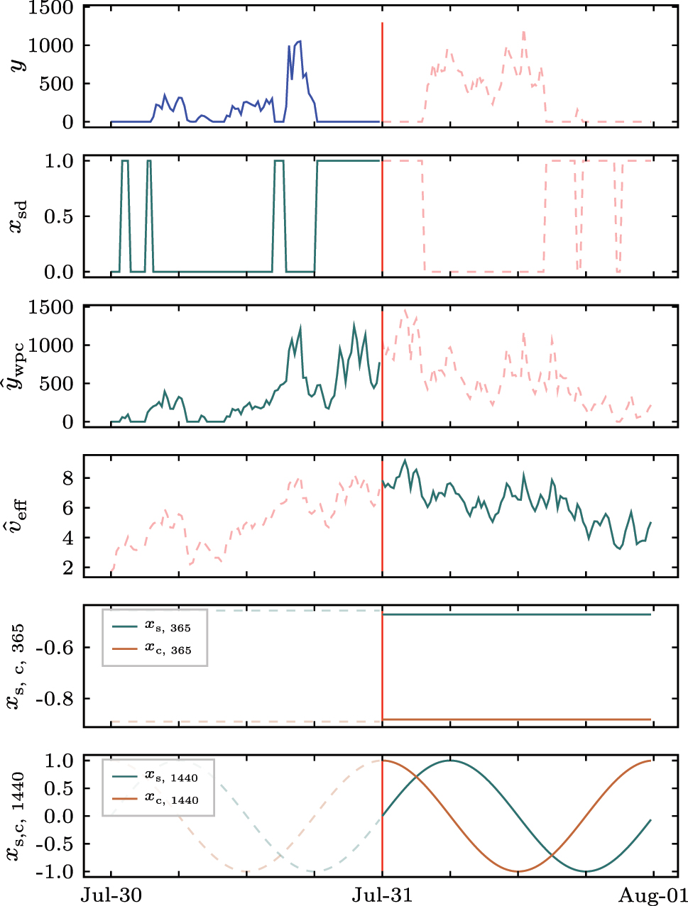
Power generation y and covariates available in the forecasting model’s future and past horizon. x
sd labels identified shutdowns in the past,
The shutdown handling method drop refers to dropping samples from the training data sub/set that are identified as abnormal operational states; and in the shutdown handling method imputation, we replace these samples with the turbine’s theoretical power generation according to the OEM WP curve (similar to [37]), see Figure 4. Finally, we combine the above principle in the shutdown handling method drop/imputation by identifying abnormal operational states, dropping these samples from the training data sub/set, and replacing them during model operation. In the operation, we only apply the data imputation to data that is available at the forecast origin, i.e., the autoregressive models’ past horizon. The calculation of the assessment metrics is always based on forecasted values and non/imputed measurements (ground truth).
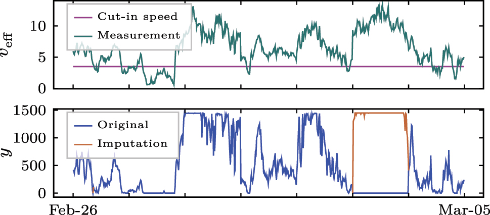
Data imputation at shutdowns with the theoretical power generation according to the turbine’s WP curve (i.e. the imputed values depend on the wind speed at hub height v eff). During shutdowns, generation y is zero although the wind speed v eff is higher than cut/in speed v eff,cut-in.
4 Evaluation
In the evaluation, state/of/the/art forecasting methods based on autoregression are compared with methods that rely solely on day/ahead weather forecasts without considering past values. First, the experimental setup for assessing the forecasting error is described. Afterward, the results are shown, and insights are provided.
4.1 Experimental setup
The experimental setup introduces the data used for evaluation and the applied evaluation strategy.
4.1.1 Data
For the evaluation, we use a real/world data set consisting of two years (2019, 2020) quarter/hourly energy metering (kWh) from two WP turbines; i.e., the time resolution is 15 min.[11] To increase interpretability, we transform the energy metering into the mean power generation time series
with the energy generation ΔE[k] (kWh) metered within the sample period t k (h). Additionally, wind speed measurements at turbines’ hub heights are available (15-min average). Both WP turbines have a peak power rating of 1,500 kWp, are located in southern Germany, and are subject to many shutdowns, see Figures 5 and 6, which are not explicitly labeled by the data provider.[12]
![Figure 5:
Identified WP turbine shutdowns with rule/based filtering [10]. Black fields represent data points at a measured wind speed greater than the cut/in speed with a power generation lower than the cut/in power. The shutdowns for WP turbine no. 1 amount to 49 % and 20 % for no. 2.](/document/doi/10.1515/auto-2024-0171/asset/graphic/j_auto-2024-0171_fig_005.jpg)
Identified WP turbine shutdowns with rule/based filtering [10]. Black fields represent data points at a measured wind speed greater than the cut/in speed with a power generation lower than the cut/in power. The shutdowns for WP turbine no. 1 amount to 49 % and 20 % for no. 2.
![Figure 6:
Data pre/processing to identify abnormal operational states [10]. Rule/based filtering identifies turbine shutdowns and LOF/based filtering identifies turbine stop/to/operation transitions and vice versa. The samples for which the wind speed at hub height is below the cut/in speed v
cut-in = 2.5 m s−1 amount to 16.7 %, while the cut/out speed v
cut-out = 25 m s−1 at which the WP turbine would be shut down for safety reasons is not reached.](/document/doi/10.1515/auto-2024-0171/asset/graphic/j_auto-2024-0171_fig_006.jpg)
Data pre/processing to identify abnormal operational states [10]. Rule/based filtering identifies turbine shutdowns and LOF/based filtering identifies turbine stop/to/operation transitions and vice versa. The samples for which the wind speed at hub height is below the cut/in speed v cut-in = 2.5 m s−1 amount to 16.7 %, while the cut/out speed v cut-out = 25 m s−1 at which the WP turbine would be shut down for safety reasons is not reached.
To perform day/ahead WP forecasting using the methods described in Section 3, we use day/ahead weather forecasts from the European Centre for Medium-Range Weather Forecasts (ECMWF) [55]. Importantly, shutdown handling in the autoregressive models’ past horizon H 1 is performed with the weather measurements available up to the forecast origin.
We split the data into a training (2019) and a test data sub/set (2020). Additionally, 20 % of the training data sub/set is hold/out for the forecasting methods DeepAR, N-HiTS, and TFT to terminate training when the loss on the hold/out data increases (early stopping).
4.1.2 Evaluation strategy
The forecasting error is evaluated under two scenarios. The first scenario concerns day/ahead WP forecasting including future shutdowns. It evaluates whether autoregressive forecasting methods can forecast both WP generation and future shutdowns. The second concerns day/ahead WP forecasts to be used for communicating the WP turbine’s availability for redispatch planning. The forecast of future shutdowns must be excluded since times of planned shutdowns are communicated via non/availability notifications. The metrics used for assessment are the normalized Mean Absolute Error (nMAE)
and the normalized Root Mean Squared Error (nRMSE)
with the forecast
For all methods, the default hyperparameter configuration of the respective implementation is used. Additionally, methods employing stochastic training algorithm (DeepAR, N-HiTS, TFT, and MLP) are run five times.
4.2 Results
In the following, the results of the two evaluation scenarios are visualized and summarized. First, the results of day/ahead WP forecasting, including shutdowns, are shown to evaluate whether future shutdowns can be forecasted. Second, the results of day/ahead WP forecasting disregarding identified shutdowns are shown to evaluate the quality of forecasts used to communicate the turbine’s availability for redispatch interventions. These results are interpreted and discussed in Section 5.
4.2.1 Shutdown handling for methods based on autoregression
Table 1 shows the impact of different shutdown handling methods on the forecasting error of state/of/the/art autoregressive DL methods (DeepAR, N-HiTS, and TFT) when considering shutdowns. With regard to WP turbine no. 1, the shutdown handling methods imputation and drop/imputation result in significantly higher forecasting errors than the others. The reason is that numerous shutdowns in the data set (see Figure 5) are imputed with OEM WP curve values (forecasting model’s past horizon), resulting in forecasts of WP generation where the turbine is actually shut down. For WP turbine no. 2, showing regular and time/dependent shutdowns (see Figure 5), considering additional explanatory variables only improves over none shutdown handling for N-HiTS, and results in particularly high errors for DeepAR. For both WP turbines, shutdown handling methods highly impact the forecasting error, but no method consistently performs best across DeepAR, N-HiTS, and TFT.
The impact of different shutdown handling methods applied to the autoregressive DL forecasting methods DeepAR, N-HiTS, and TFT on the test nMAE when considering shutdowns. Note that non-autoregressive methods (WP curve modeling, OEM WP curve, and AutoWP) generally perform worse in this scenario, as they cannot forecast shutdowns.
| Turbine no. | Error | Shutdown handling | DeepAR | N-HiTS | TFT |
|---|---|---|---|---|---|
| 1 | nMAE | None | 1.25 ± 0.08 | 0.92 ± 0.01 | 0.98 ± 0.01 |
| Explanatory variables | 1.14 ± 0.04 | 0.93 ± 0.03 | 0.94 ± 0.01 | ||
| Drop | 1.05 ± 0.09 | 0.95 ± 0.03 | 0.91 ± 0.01 | ||
| Imputation | 2.36 ± 0.36 | 2.00 ± 0.08 | 1.84 ± 0.12 | ||
| Drop-imputation | 2.61 ± 0.30 | 1.92 ± 0.03 | 1.78 ± 0.04 | ||
| 2 | nMAE | None | 1.15 ± 0.17 | 0.76 ± 0.02 | 0.81 ± 0.02 |
| Explanatory variables | 1.24 ± 0.04 | 0.73 ± 0.01 | 0.86 ± 0.01 | ||
| Drop | 1.02 ± 0.06 | 0.75 ± 0.01 | 0.81 ± 0.02 | ||
| Imputation | 0.92 ± 0.03 | 0.80 ± 0.01 | 0.79 ± 0.01 | ||
| Drop-imputation | 1.09 ± 0.04 | 0.80 ± 0.02 | 0.80 ± 0.02 | ||
| 1 | nRMSE | None | 2.42 ± 0.17 | 2.08 ± 0.02 | 2.11 ± 0.04 |
| Explanatory variables | 2.16 ± 0.09 | 2.09 ± 0.05 | 2.05 ± 0.04 | ||
| Drop | 2.12 ± 0.15 | 2.15 ± 0.05 | 1.97 ± 0.02 | ||
| Imputation | 3.33 ± 0.39 | 3.22 ± 0.15 | 2.91 ± 0.19 | ||
| Drop-imputation | 3.60 ± 0.36 | 3.07 ± 0.03 | 2.79 ± 0.06 | ||
| 2 | nRMSE | None | 1.57 ± 0.18 | 1.17 ± 0.03 | 1.22 ± 0.02 |
| Explanatory variables | 1.72 ± 0.04 | 1.10 ± 0.01 | 1.27 ± 0.02 | ||
| Drop | 1.42 ± 0.09 | 1.13 ± 0.02 | 1.20 ± 0.02 | ||
| Imputation | 1.26 ± 0.04 | 1.18 ± 0.01 | 1.15 ± 0.02 | ||
| Drop-imputation | 1.47 ± 0.06 | 1.16 ± 0.02 | 1.16 ± 0.03 |
-
The best-berforming shutdown handling method in terms of error metrics for each forecasting method is highlighted in bold.
Table 2 shows the impact of shutdown handling methods on the forecasting error of the state/of/the/art autoregressive DL methods (DeepAR, N-HiTS, and TFT) when disregarding shutdowns. With regard to WP turbine no. 1, the shutdown handling method drop results in the lowest forecasting error for DeepAR and TFT, while none shutdown handling performs best for N-HiTS. With regard to WP turbine no. 2, the shutdown handling method imputation achieves the lowest forecasting error for DeepAR and TFT, while drop/imputation achieves the lowest errors for N-HiTS. Interestingly, shutdown imputation in the past horizon with OEM WP curve values only lead to improvement for WP turbine no. 2. This is because the OEM WP curve’s forecasting error is comparably high for WP turbine no. 1, as evident in Table 3.
The impact of different shutdown handling methods applied to the autoregressive DL forecasting methods DeepAR, N-HiTS, and TFT on the test nMAE when disregarding shutdowns.
| Turbine no. | Error | Shutdown handling | DeepAR | N-HiTS | TFT |
|---|---|---|---|---|---|
| 1 | nMAE | None | 0.93 ± 0.06 | 0.73 ± 0.00 | 0.76 ± 0.01 |
| Explanatory variables | 0.86 ± 0.02 | 0.75 ± 0.02 | 0.76 ± 0.02 | ||
| Drop | 0.81 ± 0.05 | 0.75 ± 0.01 | 0.74 ± 0.01 | ||
| Imputation | 1.03 ± 0.13 | 0.88 ± 0.04 | 0.84 ± 0.05 | ||
| Drop-imputation | 1.12 ± 0.09 | 0.84 ± 0.01 | 0.83 ± 0.04 | ||
| 2 | nMAE | None | 1.00 ± 0.13 | 0.71 ± 0.02 | 0.76 ± 0.01 |
| Explanatory variables | 1.10 ± 0.03 | 0.67 ± 0.01 | 0.80 ± 0.01 | ||
| Drop | 0.90 ± 0.05 | 0.69 ± 0.01 | 0.73 ± 0.02 | ||
| Imputation | 0.77 ± 0.02 | 0.67 ± 0.01 | 0.67 ± 0.01 | ||
| Drop-imputation | 0.90 ± 0.04 | 0.66 ± 0.02 | 0.68 ± 0.02 | ||
| 1 | nRMSE | None | 1.46 ± 0.11 | 1.27 ± 0.01 | 1.31 ± 0.03 |
| Explanatory variables | 1.33 ± 0.04 | 1.29 ± 0.04 | 1.30 ± 0.03 | ||
| Drop | 1.31 ± 0.08 | 1.29 ± 0.01 | 1.26 ± 0.02 | ||
| Imputation | 1.50 ± 0.16 | 1.40 ± 0.06 | 1.32 ± 0.08 | ||
| Drop-imputation | 1.62 ± 0.11 | 1.32 ± 0.01 | 1.31 ± 0.06 | ||
| 2 | nRMSE | None | 1.35 ± 0.13 | 1.05 ± 0.03 | 1.11 ± 0.02 |
| Explanatory variables | 1.49 ± 0.03 | 0.99 ± 0.02 | 1.15 ± 0.02 | ||
| Drop | 1.23 ± 0.07 | 1.01 ± 0.02 | 1.07 ± 0.02 | ||
| Imputation | 1.06 ± 0.03 | 0.99 ± 0.01 | 0.98 ± 0.01 | ||
| Drop-imputation | 1.22 ± 0.05 | 0.97 ± 0.02 | 0.99 ± 0.03 |
-
The best-berforming shutdown handling method in terms of error metrics for each forecasting method is highlighted in bold.
Comparison of autoregressive DL forecasting methods (DeepAR, N-HiTS, and TFT) to methods based on WP curve modeling (OEM curve, AutoWP, MLP, SVR, and XGB) in terms of the test nMAE when disregarding shutdowns; results from extended evaluation of the conference paper [10].
| Turbine no. | Error | DeepAR | N-HiTS | TFT | OEM curve | AutoWP | MLP | SVR | XGB |
|---|---|---|---|---|---|---|---|---|---|
| 1 | nMAE | 0.81 ± 0.05 | 0.73 ± 0.00 | 0.74 ± 0.01 | 0.94 ± 0.00 | 0.69 ± 0.00 | 0.83 ± 0.01 | 0.70 ± 0.00 | 0.84 ± 0.00 |
| 2 | 0.77 ± 0.02 | 0.66 ± 0.02 | 0.67 ± 0.01 | 0.67 ± 0.00 | 0.61 ± 0.00 | 0.69 ± 0.01 | 0.64 ± 0.00 | 0.74 ± 0.00 | |
| 1 | nRMSE | 1.31 ± 0.08 | 1.27 ± 0.01 | 1.26 ± 0.02 | 1.57 ± 0.00 | 1.20 ± 0.00 | 1.15 ± 0.01 | 1.11 ± 0.00 | 1.22 ± 0.00 |
| 2 | 1.06 ± 0.03 | 0.97 ± 0.02 | 0.98 ± 0.01 | 1.07 ± 0.00 | 0.93 ± 0.00 | 0.92 ± 0.00 | 0.93 ± 0.00 | 1.01 ± 0.00 |
-
The best-berforming shutdown handling method in terms of error metrics for each forecasting method is highlighted in bold.
4.2.2 Comparison of autoregressive and WP curve-based methods
Table 3 compares the forecasting error of the autoregressive DL methods DeepAR, N-HiTS and TFT (using the respective best/performing shutdown handling method) with WP curve modeling-based forecasting methods. Notably, even with the optimal shutdown handling method, the autoregressive DL methods underperform compared to the methods based on WP curve modeling. Within the WP curve modeling methods, AutoWP, MLP, and SVR achieve similar forecasting errors. While AutoWP achieves the lowest nMAE for both turbines, the SVR achieves the lowest nRMSE for WP turbine no. 1, and the MLP for no. 2, see Table 3.[13]
4.3 Insights
In the following, the specific insights of the evaluation are given. Figure 7 provides an exemplary visual comparison of WP generation forecasts for WP turbine no. 2. Apart from the WP generation, also the wind speed measurement at hub height and the height/corrected wind speed forecast from ECMWF is shown. This exemplary comparison reveals that the wind speed forecast has a different influence on the resulting WP generation forecast from N-HiTS, AutoWP, and MLP. Unlike AutoWP, which relies only on the height/corrected wind speed forecast, the MLP additionally takes the wind direction, air temperature, and atmospheric pressure into account, and N-HiTS furthermore considers past WP generation measurements. Figure 8 illustrates this in greater detail, plotting the WP generation measurement y and forecast
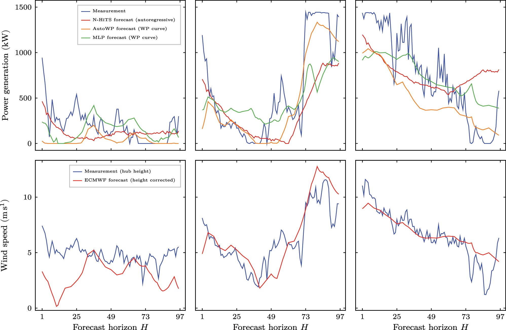
Exemplary comparison of WP forecasts for WP turbine no. 2 using N-HiTS (autoregressive), AutoWP and MLP (WP curve modeling) on days without shutdowns. While methods based on WP curve modeling are only based on weather forecasts (ECMWF), autoregressive methods also consider past WP generation measurements when making forecasts. Legend of first column of a row applies to all columns in the row.
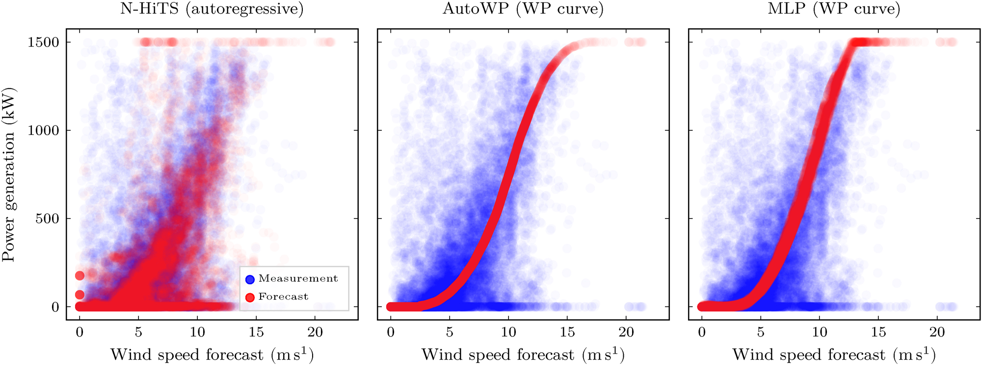
Relationship between wind speed forecast (ECMWF) and WP generation forecasts (N-HiTS, AutoWP, MLP) for WP turbine no. 2 when disregarding shutdowns. AutoWP relies only on the height/corrected wind speed forecast, the MLP is trained using the forecasts of wind speed and direction, temperature and air pressure, and N-HiTS additionally considers past WP generation measurements. No WP generation despite moderate and high wind speeds are not shutdowns (already filtered out) but result from the error in the weather forecast, i.e., the wind speed forecast is above the cut/in speed while the realized wind speed is underneath. Legend of first column applies to all columns.
5 Discussion
In the following, the results of the two evaluation scenarios are discussed, the study’s limitations are summarized, and recommendations are derived.
5.1 Shutdown handling for methods based on autoregression
With regard to the first scenario, we observe that shutdown handling methods significantly impact the forecasting error. However, none of them consistently performs best across the autoregressive DL methods DeepAR, N-HiTS, and TFT. The already high computational training effort for these forecasting methods is further compounded by the need to identifying the best shutdown handling techniques, making model design even more resource/intensive. This limits the scalable use and model deployment to a large number of individual WP turbines.
5.2 Comparison of autoregressive and WP curve-based methods
With regard to the second scenario, the results show that even with the best/performing shutdown handling method, the considered autoregressive DL methods do not improve over WP curve modeling methods on the given data set. Importantly, WP curve modeling methods are static, i.e., only use day/ahead weather forecasts and thus cannot forecast regular shutdowns. Such regular shutdowns can be considered either by having PK of timed shutdowns or by designing a separate classification model that estimates whether the WP turbine is in operation or shut down. However, such a modeling approach requires a data set in which regular and irregular shutdowns are labeled. The challenge of distinguishing between regular and irregular shutdowns becomes obvious in Figure 5, where recurring shutdown patterns are visible that are not strictly regular and may be interspersed with irregular shutdowns.
5.3 Limitations
Although the data of two WP turbines with different shutdown patterns are considered, the data set is too small for drawing generalized conclusions. Nevertheless, the evaluation reveals major issues for the scalable application of autoregressive DL methods regarding redispatch planning. For such forecasts, computationally efficient WP curve modeling approaches are recommended. In this context, a parametrized and normalized WP curve with a few key parameters (e.g., cut/in, cut/out, rated power, and shape parameters) might offer an interpretable and computationally efficient alternative to the ensemble-based AutoWP method. Although the weights derived in the AutoWP approach offer a degree of interpretability, a parametric model with explicit key parameters may provide greater transparency in representing wind power behavior. A comparison between the AutoWP ensemble and such a parametric approach using classical least/squares parameter estimation remains an interesting direction for future work. Another limitation relates to the potentially untapped potential of HPO to reduce forecasting errors. However, even if HPO could reduce forecasting errors of autoregressive DL methods, it would further add to the computational effort required for the model design. To improve the performance of the autoregressive DL methods, labeled data sets would be required to distinguish between regular and irregular shutdowns.
5.4 Benefits
AutoWP can represent different site conditions characterized by terrain/induced air turbulence, leveraging an ensemble of different WP curves. More precisely, these site conditions influence the wind speed at which the WP turbine reaches its peak power output. These site conditions can differ greatly from the ones under which the OEM WP curve was determined, potentially resulting in a high forecasting error when using the OEM WP curve (as shown in the evaluation). Although a site/specific WP curve can also be considered when using ML methods, AutoWP is advantageous because physical constraints in the WP generation are implicitly considered, and only a few samples are required to train the model. This scalability is crucial for the model deployment to a large number of distributed onshore WP turbines to serve smart grid applications like redispatch planning.
6 Conclusion and outlook
Automated forecasting of locally distributed WP generation is crucial for various smart grid applications in light of redispatch planning. However, forecasting future shutdowns based on past redispatch interventions is evidently undesirable. Therefore, this paper increases awareness regarding this issue by comparing state/of/the/art forecasting methods on data sets containing regular and irregular shutdowns. We observe that autoregressive DL methods require time/consuming data pre-processing for training and during operation to handle WP turbine shutdowns. In contrast, static WP curve modeling methods that do not consider past values to make a forecast only require training data cleaning. Within WP curve modeling methods, AutoWP [10] is especially beneficial since it is computationally efficient, implicitly includes PK about physical limitations in WP generation, and achieves competitive performance.
Future work could address the stated limitations by extending the evaluation to a larger data set, labeled regarding regular and irregular WP turbine shutdowns. With such a data set, a separate classification model could be designed that predicts whether the WP turbine is in operation or shut down. Additionally, future research could compare the AutoWP ensemble approach with a parametrized and normalized WP curve using classical least/squares parameter estimation, to shed light on trade/offs between interpretability, accuracy, and computational efficiency.
-
Research ethics: Not applicable.
-
Informed consent: Not applicable.
-
Author contributions: All authors have accepted responsibility for the entire content of this manuscript and approved its submission.
-
Use of Large Language Models, AI and Machine Learning Tools: None declared.
-
Research funding: This project is funded by the Helmholtz Association under the Program “Energy System Design”, the German Research Foundation (DFG) as part of the Research Training Group 2153 “Energy Status Data: Informatics Methods for its Collection, Analysis and Exploitation” and the Helmholtz Associations Initiative and Networking Fund through Helmholtz AI, and is supported by the HAICORE@KIT partition. Furthermore, the authors thank Stadtwerke Karlsruhe Netzservice GmbH (Karlsruhe, Germany) for the data required for this work.
-
Data availability: Not applicable.
References
[1] F. Salm, M. Oettmeier, and P. Rönsch, “The new redispatch and the impact on energy management in districts,” in 2022 18th International Conference on the European Energy Market (EEM), 2022, pp. 1–4.10.1109/EEM54602.2022.9921014Suche in Google Scholar
[2] R. Meka, A. Alaeddini, and K. Bhaganagar, “A robust deep learning framework for short-term wind power forecast of a full-scale wind farm using atmospheric variables,” Energy, vol. 221, 2021, Art. no. 119759. https://doi.org/10.1016/j.energy.2021.119759.Suche in Google Scholar
[3] Z. Wang, L. Wang, and C. Huang, “A fast abnormal data cleaning algorithm for performance evaluation of wind turbine,” IEEE Trans. Instrum. Meas., vol. 70, pp. 1–12, 2021. https://doi.org/10.1109/TIM.2020.3044719.Suche in Google Scholar
[4] Y. Su, et al.., “Wind power curve data cleaning algorithm via image thresholding,” in 2019 IEEE International Conference on Robotics and Biomimetics (ROBIO), 2019, pp. 1198–1203.10.1109/ROBIO49542.2019.8961448Suche in Google Scholar
[5] Z. Luo, C. Fang, C. Liu, and S. Liu, “Method for cleaning abnormal data of wind turbine power curve based on density clustering and boundary extraction,” IEEE Trans. Sustain. Energy, vol. 13, no. 2, pp. 1147–1159, 2022. https://doi.org/10.1109/TSTE.2021.3138757.Suche in Google Scholar
[6] S. Klaiber, et al.., “A contribution to the load forecast of price elastic consumption behaviour,” in 2015 IEEE Eindhoven PowerTech, 2015, pp. 1–6.10.1109/PTC.2015.7232548Suche in Google Scholar
[7] D. Salinas, V. Flunkert, J. Gasthaus, and T. Januschowski, “DeepAR: probabilistic forecasting with autoregressive recurrent networks,” Int. J. Forecast., vol. 36, no. 3, pp. 1181–1191, 2020. https://doi.org/10.1016/j.ijforecast.2019.07.001.Suche in Google Scholar
[8] C. Challú, K. G. Olivares, B. N. Oreshkin, F. Garza Ramirez, M. Mergenthaler Canseco, and A. Dubrawski, “N-HiTS: neural hierarchical interpolation for time series forecasting,” Proc. AAAI Conf. Artif. Intell., vol. 37, no. 6, pp. 6989–6997, 2023. https://doi.org/10.1609/aaai.v37i6.25854.Suche in Google Scholar
[9] B. Lim, S. Ö. Arık, N. Loeff, and T. Pfister, “Temporal fusion transformers for interpretable multi-horizon time series forecasting,” Int. J. Forecast., vol. 37, no. 4, pp. 1748–1764, 2021. https://doi.org/10.1016/j.ijforecast.2021.03.012.Suche in Google Scholar
[10] S. Meisenbacher, et al.., “AutoWP: automated wind power forecasts with limited computing resources using an ensemble of diverse wind power curves,” in Proceedings of the 34. Workshop Computational Intelligence, Berlin, Germany, KIT Scientific Publishing, 2024, pp. 1–20.10.58895/ksp//1000174544-1Suche in Google Scholar
[11] S. Meisenbacher, et al.., “Review of automated time series forecasting pipelines,” WIREs Data Min. Knowl. Discov., vol. 12, no. 6, 2022, Art. no. e1475. https://doi.org/10.1002/widm.1475.Suche in Google Scholar
[12] H. Schulte, “Modeling of wind turbines,” in Advanced Control of Grid-Integrated Renewable Energy Power Plants, Hoboken, USA, John Wiley & Sons, Ltd, 2024, pp. 15–61. Chap. 2.10.1002/9781119701415.ch2Suche in Google Scholar
[13] S. Meisenbacher, et al.., “AutoPV: automated photovoltaic forecasts with limited information using an ensemble of pre-trained models,” in Proceedings of the 14th ACM International Conference on Future Energy Systems. e-Energy ’23, Orlando, USA, Association for Computing Machinery, 2023, pp. 386–414.10.1145/3575813.3597348Suche in Google Scholar
[14] C. Sweeney, R. J. Bessa, J. Browell, and P. Pinson, “The future of forecasting for renewable energy,” WIREs Energy Environ., vol. 9, no. 2, 2020, Art. no. e365. https://doi.org/10.1002/wene.365.Suche in Google Scholar
[15] M. López Santos, X. García-Santiago, F. Echevarría Camarero, G. Blázquez Gil, and P. Carrasco Ortega, “Application of temporal fusion transformer for day-ahead PV power forecasting,” Energies, vol. 15, no. 14, p. 5232, 2022. https://doi.org/10.3390/en15145232.Suche in Google Scholar
[16] L. van Heerden, C. van Staden, and H. Vermeulen, “Temporal fusion transformer for day-ahead wind power forecasting in the South African context,” in 2023 IEEE International Conference on Environment and Electrical Engineering and 2023 IEEE Industrial and Commercial Power Systems Europe (EEEIC/I&CPS Europe), 2023, pp. 1–5.10.1109/EEEIC/ICPSEurope57605.2023.10194737Suche in Google Scholar
[17] S. Rajagopalan and S. Santoso, “Wind power forecasting and error analysis using the autoregressive moving average modeling,” in 2009 IEEE Power & Energy Society General Meeting, 2009, pp. 1–6.10.1109/PES.2009.5276019Suche in Google Scholar
[18] B.-M. Hodge, A. Zeiler, D. Brooks, G. Blau, J. Pekny, and G. Reklatis, “Improved wind power forecasting with ARIMA models,” in 21st European Symposium on Computer Aided Process Engineering, Computer Aided Chemical Engineering, vol. 29, E. Pistikopoulos, M. Georgiadis, and A. Kokossis, Eds., Elsevier, 2011, pp. 1789–1793.10.1016/B978-0-444-54298-4.50136-7Suche in Google Scholar
[19] E. Ahn and J. Hur, “A short-term forecasting of wind power outputs using the enhanced wavelet transform and arimax techniques,” Renewable Energy, vol. 212, pp. 394–402, 2023. https://doi.org/10.1016/j.renene.2023.05.048.Suche in Google Scholar
[20] R. A. Sobolewski, M. T. Tchakorom, and R. Couturier, “Gradient boosting-based approach for short- and medium-term wind turbine output power prediction,” Renewable Energy, vol. 203, pp. 142–160, 2023. https://doi.org/10.1016/j.renene.2022.12.040.Suche in Google Scholar
[21] A. Lahouar and J. Ben Hadj Slama, “Hour-ahead wind power forecast based on random forests,” Renewable Energy, vol. 109, pp. 529–541, 2017. https://doi.org/10.1016/j.renene.2017.03.064.Suche in Google Scholar
[22] Y. Liu, et al.., “Wind power short-term prediction based on LSTM and discrete wavelet transform,” Appl. Sci., vol. 9, no. 6, p. 1108, 2019. https://doi.org/10.3390/app9061108.Suche in Google Scholar
[23] B. Zhou, X. Ma, Y. Luo, and D. Yang, “Wind power prediction based on LSTM networks and nonparametric kernel density estimation,” IEEE Access, vol. 7, pp. 165279–165292, 2019. https://doi.org/10.1109/ACCESS.2019.2952555.Suche in Google Scholar
[24] R. Zhu, W. Liao, and Y. Wang, “Short-term prediction for wind power based on temporal convolutional network,” Energy Rep., vol. 6, pp. 424–429, 2020. https://doi.org/10.1016/j.egyr.2020.11.219.Suche in Google Scholar
[25] F. Shahid, A. Zameer, and M. Muneeb, “A novel genetic LSTM model for wind power forecast,” Energy, vol. 223, 2021, Art. no. 120069. https://doi.org/10.1016/j.energy.2021.120069.Suche in Google Scholar
[26] P. Arora, S. M. J. Jalali, S. Ahmadian, B. K. Panigrahi, P. N. Suganthan, and A. Khosravi, “Probabilistic wind power forecasting using optimized deep auto-regressive recurrent neural networks,” IEEE Trans. Ind. Inform., vol. 19, no. 3, pp. 2814–2825, 2023. https://doi.org/10.1109/TII.2022.3160696.Suche in Google Scholar
[27] S. Sun, Y. Liu, Q. Li, T. Wang, and F. Chu, “Short-term multi-step wind power forecasting based on spatio-temporal correlations and transformer neural networks,” Energy Convers. Manage., vol. 283, 2023, Art. no. 116916. https://doi.org/10.1016/j.enconman.2023.116916.Suche in Google Scholar
[28] Y. Hu, H. Liu, S. Wu, Y. Zhao, Z. Wang, and X. Liu, “Temporal collaborative attention for wind power forecasting,” Appl. Energy, vol. 357, 2024, Art. no. 122502. https://doi.org/10.1016/j.apenergy.2023.122502.Suche in Google Scholar
[29] S. Xu, et al.., “A multi-step wind power group forecasting seq2seq architecture with spatial-temporal feature fusion and numerical weather prediction correction,” Energy, vol. 291, 2024, Art. no. 130352. https://doi.org/10.1016/j.energy.2024.130352.Suche in Google Scholar
[30] S. Mo, H. Wang, B. Li, Z. Xue, S. Fan, and X. Liu, “Powerformer: a temporal-based transformer model for wind power forecasting,” Energy Rep., vol. 11, pp. 736–744, 2024. https://doi.org/10.1016/j.egyr.2023.12.030.Suche in Google Scholar
[31] M. Lydia, S. S. Kumar, A. I. Selvakumar, and G. E. Prem Kumar, “A comprehensive review on wind turbine power curve modeling techniques,” Renewable Sustainable Energy Rev., vol. 30, pp. 452–460, 2014. https://doi.org/10.1016/j.rser.2013.10.030.Suche in Google Scholar
[32] C. Carrillo, A. Obando Montaño, J. Cidrás, and E. Díaz-Dorado, “Review of power curve modelling for wind turbines,” Renewable Sustainable Energy Rev., vol. 21, pp. 572–581, 2013. https://doi.org/10.1016/j.rser.2013.01.012.Suche in Google Scholar
[33] M. Lydia, A. I. Selvakumar, S. S. Kumar, and G. E. P. Kumar, “Advanced algorithms for wind turbine power curve modeling,” IEEE Trans. Sustain. Energy, vol. 4, no. 3, pp. 827–835, 2013. https://doi.org/10.1109/TSTE.2013.2247641.Suche in Google Scholar
[34] R. K. Pandit, D. Infield, and A. Kolios, “Comparison of advanced non-parametric models for wind turbine power curves,” IET Renew. Power Gener., vol. 13, no. 9, pp. 1503–1510, 2019. https://doi.org/10.1049/iet-rpg.2018.5728.Suche in Google Scholar
[35] S. R. Moreno, L. D. S. Coelho, H. V. Ayala, and V. C. Mariani, “Wind turbines anomaly detection based on power curves and ensemble learning,” IET Renew. Power Gener., vol. 14, no. 19, pp. 4086–4093, 2020. https://doi.org/10.1049/iet-rpg.2020.0224.Suche in Google Scholar
[36] U. Singh, M. Rizwan, M. Alaraj, and I. Alsaidan, “A machine learning-based gradient boosting regression approach for wind power production forecasting: a step towards smart grid environments,” Energies, vol. 14, no. 16, p. 5196, 2021. https://doi.org/10.3390/en14165196.Suche in Google Scholar
[37] Y. Wang, Q. Hu, D. Srinivasan, and Z. Wang, “Wind power curve modeling and wind power forecasting with inconsistent data,” IEEE Trans. Sustain. Energy, vol. 10, no. 1, pp. 16–25, 2019. https://doi.org/10.1109/TSTE.2018.2820198.Suche in Google Scholar
[38] S. Li, D. Wunsch, E. O’Hair, and M. Giesselmann, “Using neural networks to estimate wind turbine power generation,” IEEE Trans. Energy Convers., vol. 16, no. 3, pp. 276–282, 2001. https://doi.org/10.1109/60.937208.Suche in Google Scholar
[39] M. Schlechtingen, I. F. Santos, and S. Achiche, “Using data-mining approaches for wind turbine power curve monitoring: a comparative study,” IEEE Trans. Sustain. Energy, vol. 4, no. 3, pp. 671–679, 2013. https://doi.org/10.1109/TSTE.2013.2241797.Suche in Google Scholar
[40] M. Á. Rodríguez-López, E. Cerdá, and P. D. Rio, “Modeling wind-turbine power curves: effects of environmental temperature on wind energy generation,” Energies, vol. 13, no. 18, p. 4941, 2020. https://doi.org/10.3390/en13184941.Suche in Google Scholar
[41] R. Morrison, X. L. Liu, and Z. Lin, “Anomaly detection in wind turbine SCADA data for power curve cleaning,” Renewable Energy, vol. 184, pp. 473–486, 2022. https://doi.org/10.1016/j.renene.2021.11.118.Suche in Google Scholar
[42] P. Mucchielli, B. Bhowmik, B. Ghosh, and V. Pakrashi, “Real-time accurate detection of wind turbine downtime – an Irish perspective,” Renewable Energy, vol. 179, pp. 1969–1989, 2021. https://doi.org/10.1016/j.renene.2021.07.139.Suche in Google Scholar
[43] J. Á. González Ordiano, S. Waczowicz, V. Hagenmeyer, and R. Mikut, “Energy forecasting tools and services,” WIREs Data Min. Knowl. Discov., vol. 8, no. 2, 2018, Art. no. e1235. https://doi.org/10.1002/widm.1235.Suche in Google Scholar
[44] J. Beitner, PyTorch Forecasting, 2020. https://towardsdatascience.com/introducing-pytorch-forecasting-64de99b9ef46 [Accessed: Feb. 01, 2021].Suche in Google Scholar
[45] S. Hochreiter and J. Schmidhuber, “Long short-term memory,” Neural Comput., vol. 9, no. 8, pp. 1735–1780, 1997. https://doi.org/10.1162/neco.1997.9.8.1735.Suche in Google Scholar PubMed
[46] A. Vaswani, et al.., “Attention is all you need,” in Advances in Neural Information Processing Systems, vol. 30, I. Guyon, et al.., Eds., Curran Associates, Inc., 2017.Suche in Google Scholar
[47] D. Etling, “Die atmosphärische Grenzschicht,” in Theoretische Meteorologie: Eine Einführung, Berlin, Heidelberg, Germany, Springer-Verlag, 2004, pp. 297–340. Chap. 21.Suche in Google Scholar
[48] C. Jung and D. Schindler, “The role of the power law exponent in wind energy assessment: a global analysis,” Int. J. Energy Res., vol. 45, no. 6, pp. 8484–8496, 2021. https://doi.org/10.1002/er.6382.Suche in Google Scholar
[49] G. M. Masters, “Wind power systems,” in Renewable and Efficient Electric Power Systems, Chichester, UK, John Wiley & Sons, Ltd, 2004, pp. 307–383. Chap. 6.10.1002/0471668826.ch6Suche in Google Scholar
[50] S. Meisenbacher, et al.., “Concepts for automated machine learning in smart grid applications,” in Proceedings of the 31. Workshop Computational Intelligence, Berlin, Germany, KIT Scientific Publishing, 2021, pp. 11–35.10.58895/ksp/1000138532-2Suche in Google Scholar
[51] S. A. Hsu, E. A. Meindl, and D. B. Gilhousen, “Determining the power-law wind-profile exponent under near-neutral stability conditions at sea,” J. Appl. Meteorol. Climatol., vol. 33, no. 6, pp. 757–765, 1994. https://doi.org/10.1175/1520-0450(1994)033<0757:DTPLWP>2.0.CO;2.10.1175/1520-0450(1994)033<0757:DTPLWP>2.0.CO;2Suche in Google Scholar
[52] M. Petersen, J. Huber, and C. Hofmann, Wind Turbine Library, Further contributors: Ludee, jh-RLI, 2019. Available at: https://openenergy-platform.org/dataedit/view/model_draft/wind_turbine_library.Suche in Google Scholar
[53] L. Svenningsen, Power Curve Air Density Correction and Other Power Curve Options in WindPRO, Aalborg, Denmark, EMD International A/S, 2010.Suche in Google Scholar
[54] P. Virtanen, et al.., “SciPy 1.0: fundamental algorithms for scientific computing in python,” Nat. Methods, vol. 17, pp. 261–272, 2020. https://doi.org/10.1038/s41592-019-0686-2.Suche in Google Scholar
[55] European Centre for Medium-Range Weather Forecasts (ECMWF), Meteorological Archival and Retrieval System (MARS), 2023. https://confluence.ecmwf.int/display/CEMS/MARS [Accessed: Mar. 06, 2024].Suche in Google Scholar
© 2025 the author(s), published by De Gruyter, Berlin/Boston
This work is licensed under the Creative Commons Attribution 4.0 International License.
Artikel in diesem Heft
- Frontmatter
- Editorial
- Selected contributions from the workshops “Computational Intelligence” in 2023 and 2024
- Methods
- Nonlinear system categorization for structural data mining with state space models
- Incorporation of structural properties of the response surface into oblique model trees
- Takagi-Sugeno based model reference control for wind turbine systems in frequency containment scenarios
- On autoregressive deep learning models for day-ahead wind power forecasts with irregular shutdowns due to redispatching
- Applications
- Efficiently determining the effect of data set size on autoencoder-based metamodels for structural design optimization
- Kalibriermodellerstellung und Merkmalsselektion für die mikromagnetische Materialcharakterisierung mittels maschineller Lernverfahren
- Investigating quality inconsistencies in the ultra-high performance concrete manufacturing process using a search-space constrained non-dominated sorting genetic algorithm II
- EAP4EMSIG – enhancing event-driven microscopy for microfluidic single-cell analysis