Investigating quality inconsistencies in the ultra-high performance concrete manufacturing process using a search-space constrained non-dominated sorting genetic algorithm II
-
Farzad Rezazadeh
 ,
Amin Abrishambaf
,
Amin Abrishambaf

Abstract
Ultra-high performance concrete (UHPC) surpasses conventional concrete in performance. However, ensuring consistent mechanical properties during production, even with identical recipes, remains challenging. Using experimental data, this study investigates how material quality, environmental conditions, measurement errors in material dosing, and mixing and curing conditions influence the mechanical properties of UHPC. This broad scope of influencing factors and production conditions increases data dimensionality and, coupled with the high cost of UHPC experiments, results in a sparse dataset. Traditional evolutionary algorithms, though effective in feature selection, struggle with high-dimensional small-sized datasets. To address this, a search-space-constraining method for the non-dominated sorting genetic algorithm II (NSGA-II) is introduced, incorporating domain-specific knowledge into population initialization to reduce dimensionality and thus enhance prediction accuracy and solution stability. Comparative evaluations using various machine learning algorithms on the UHPC dataset demonstrate that population initialization to constrain the search space of NSGA-II outperforms the standard NSGA-II. Finally, the significance of each examined factor in the UHPC manufacturing process for the properties of the final product is discussed.
Zusammenfassung
Ultra-Hochleistungsbeton (UHPC) übertrifft konventionelle Betone hinsichtlich der Leistungsfähigkeit. Die Gewährleistung reproduzierbarer mechanischer Eigenschaften bleibt jedoch selbst bei identischen Rezepturen herausfordernd. Auf Basis experimenteller Daten untersucht diese Studie den Einfluss von Materialqualität, Umgebungsbedingungen, Messfehlern in der Materialdosierung sowie Misch- und Nachbehandlungsbedingungen auf die mechanischen Eigenschaften von UHPC. Die Vielzahl potenzieller Einflussgrößen und Prozessbedingungen führt zu hoher Dimensionalität; zugleich begrenzen die hohen Versuchskosten die Stichprobengröße. Es liegt daher ein hochdimensionaler Datensatz mit geringer Fallzahl vor. Klassische evolutionäre Algorithmen sind zwar in der Merkmalsauswahl leistungsfähig, stoßen bei hochdimensionalen, kleinen Datensätzen jedoch an Grenzen. Zur Abhilfe wird eine suchraumbeschränkende Variante des Non-Dominated Sorting Genetic Algorithm II (NSGA-II) vorgestellt, die domänenspezifisches Wissen bereits in der Populationsinitialisierung einbindet, die effektive Dimensionalität reduziert und damit Vorhersagegenauigkeit sowie Lösungsstabilität erhöht. Vergleichende Auswertungen mit verschiedenen Machine-Learning-Verfahren auf dem UHPC-Datensatz belegen Vorteile gegenüber dem Standard-NSGA-II hinsichtlich Vorhersagegüte und Lösungsstabilität. Abschließend wird die relative Bedeutung der betrachteten Einflussfaktoren im UHPC-Herstellprozess für die Eigenschaften des Endprodukts diskutiert.
1 Introduction
Ultra-high performance concrete (UHPC) is an advanced cement-based composite known for its exceptional mechanical strength and durability. Typically, it contains a high volume of short steel fibers (approximately 2 % by volume) distributed within a dense matrix with a low water-to-binder ratio, often incorporating silica fume. This composition enables UHPC to exhibit uniaxial tensile hardening behavior, which promotes stable microcracks and excellent transport properties even under demanding conditions. These characteristics make UHPC suitable for bridge construction, structural strengthening, and waterproofing. However, the high cement and silica fume content increases production costs and contributes significantly to the CO2 footprint [1].
Additionally, the production process for UHPC is highly sensitive [2]. Minor deviations from the recipe or changes in environmental conditions can affect consistency and mechanical behavior, leading to higher waste. To address these issues, the construction industry requires an advanced support system capable of predicting UHPC properties in real time, enhancing quality control, reducing waste, improving product quality, and lowering costs.
To date, most investigations of the UHPC manufacturing process have focused on individual factors rather than the interactions among all relevant ones. Using the publicly available dataset [3], variations of a reference UHPC recipe and production conditions are systematically evaluated. Specifically, the impacts of raw material properties (e.g. impurities, particle size distribution), dosing system errors, energy consumption during mixing, and environmental conditions (affecting both raw materials and specimen curing) on UHPC quality are assessed (see Figure 1). By understanding the most influential and informative factors in the UHPC production process, practitioners can predict the quality of the final product early, before the costly curing process.

Ultra-high performance concrete (UHPC) manufacturing process. Production and testing procedures, influencing factors, and key considerations regarding the impact of material quality, particle size distributions, measurement errors, and environmental conditions on final UHPC mechanical performance. (El.: Electrical, CS: Compressive strength, FS: Flexural strength).
Modeling the UHPC manufacturing process poses significant challenges due to the complex physical and chemical subprocesses involved. Generating data for one experimental point requires 28 days, making the process time-consuming and costly. This data generation, coupled with the large number of key factors in this production process, results in a sparse dataset [3]. High dimensionality and small sample size further complicate modeling efforts. In such cases, the feature selection process plays a crucial role. Standard feature selection methods [4], such as sequential feature selection and recursive feature elimination, often struggle to detect patterns in high-dimensional datasets; they frequently miss critical relationships and become trapped in local minima [5], [6]. Although evolutionary multiobjective feature selection methods can outperform greedy search-based approaches, they are less effective for high-dimensional, small-sized datasets.
To overcome these difficulties, this contribution focuses on a multi-step dimensionality reduction approach. By incorporating domain knowledge into the initial population of the standard non-dominated sorting genetic algorithm II (NSGA-II) [7], the prediction accuracy and solution stability are enhanced. This population-initialization method effectively addresses the challenges of high dimensionality and small sample size in evolutionary multiobjective feature selection, improving prediction performance, solution stability, and interpretability in high-dimensional datasets with small sample sizes.
The remainder of this paper is organized as follows: Section 2 reviews parameter studies and mechanical property prediction for concrete, along with a background on evolutionary multiobjective feature selection. Section 3 details the proposed modeling pipeline for UHPC production. Section 4 analyzes the effect of the introduced population-initialization method, which constrains the search space, on NSGA-II. Finally, Section 5 concludes the study and provides insights for future research.
2 Related work
2.1 Predicting concrete mechanical properties
Predicting the compressive strength (CS) of concrete, particularly its 28-day CS, has traditionally relied on empirical relationships [8] and, more recently, machine learning techniques [9], [10]. The initial obstacle to adopting machine learning techniques in concrete research is the scarcity of comprehensive, high-quality datasets. The datasets on Compressive Strength [11] and Slump Flow Test [12], collected by Yeh from diverse research sources, are commonly used [13], [14]. These generally focus on the impact of mixing proportions on high-performance concrete. Since the datasets are compiled from diverse sources, they are susceptible to inherent redundancies and inconsistencies.
Nguyen et al. [15] employed the XGB algorithm to predict CS of UHPC using a dataset of 931 mix formulations derived from both laboratory experiments and the existing literature. However, the dataset does not incorporate potential uncertainties in material quality, dosing, and environmental conditions.
Aylas-Paredes et al. [16] built a 1,300-entry UHPC dataset from more than 55 studies and trained a random forest (RF) and a three-layer artificial neural network (ANN) to predict the 28-day strength. Hyperparameters were tuned by 10-fold cross-validation (CV), but accuracy came from a single 75 %/25 % train–test split, risking sampling and initialization bias. Undocumented mixing, curing and storage differences across labs further threaten generalizability.
Wakjira et al. [17] trimmed Abellán-García’s 931-mix UHPC [18] archive to 540 mixes by deleting entries with missing data and keeping only 10 compositional variables, omitting all processing details (e.g. curing and batching temperature). They trained decision-tree, GBM and XGB models and stacked them with a linear-SVR meta learner, but validated the system on just one random 80 %/20 % train–test split with no repeated initializations. Consequently, both the reported accuracy and the multiobjective Pareto fronts may vary with a different split, and ensemble diversity is limited because each base learner is tree-based [19].
Designing a pipeline for the concrete production process with sparse data has been seldom addressed [20]. Recently, Golafshani et al. [21] proposed a pipeline for modeling concrete production and optimizing mixtures that investigates a framework for the low-carbon mix design of recycled aggregate concrete with supplementary cementitious materials using machine learning.
Despite progress in predicting concrete mechanical properties, notable challenges persist [22]. These include limited data coverage of material quality, measurement errors, and mixing and curing conditions – factors that necessitate a holistic perspective on the production process. Even minor variations in these variables can lead to inconsistencies in UHPC quality, despite using identical recipes [23]. Additional hurdles include systematic data generation, feature selection methods that fail under high dimensionality and limited sample sizes, inadequate training-testing strategies, and a narrow range of investigated algorithms. To address these gaps, this study investigates the effects of material quality, uncertainties in material dosing and particle size distribution, as well as mixing and environmental conditions on final mechanical properties. By leveraging the developed multiobjective feature selection method and a diverse set of 10 machine learning algorithms and employing a leave-one-out cross-validation (LOOCV) [24] training-testing strategy – coupled with multiple initializations – the proposed methodology ensures reliable predictions of UHPC mechanical properties.
2.2 Evolutionary multiobjective feature selection
Feature selection (FS) is crucial in machine learning, particularly for high-dimensional datasets with small sample sizes. It enhances model interpretability, mitigates overfitting, and improves prediction accuracy by discarding irrelevant or redundant features. Traditionally, FS methods – filter, wrapper, and embedded – may select redundant features, exhibit nesting effects, or become trapped in local optima, especially in complex, high-dimensional domains [5], [6].
Evolutionary multiobjective feature selection (EMOFS) has been studied for several decades [25]. It excels in global optimization and can handle high-dimensional data; however, it generally requires large datasets. For complex, sparse datasets, the intrinsic randomness of evolutionary processes often leads to unstable outcomes. As a result, EMOFS has primarily been employed for large-scale classification tasks [26], [27], [28], [29]. One way to address this challenge is incorporating prior knowledge into the FS process [30]. EMOFS methodologies can integrate domain expertise at multiple design stages, including solution representation, evaluation metrics, initialization strategies, offspring generation methods, environmental selection, and decision-making [6]. Kropp et al. [31] propose a Sparse Population Sampling technique, seeding the population with sparse initial solutions and thus leveraging a form of prior knowledge. Xu et al. [32] employ duplication analysis to simplify FS by exploiting patterns of feature redundancy. Song et al. [33] group features based on correlations before using particle swarm optimization, thereby harnessing prior knowledge of feature relationships. Ren et al. [34] develop an algorithm for sparse optimization that indirectly integrates domain insights by emphasizing the distribution of non-zero elements. Likewise, Wang et al. [35] apply multiobjective differential evolution to balance feature minimization and classification performance, implying an indirect use of domain-specific feature importance. Vatolkin et al. [25] apply EMOFS, optimizing trade-offs between classification error and the number of features. Follow-up studies [36] further generalized this approach to multiple objective pairs and scenarios. These works show the efficacy of EMOFS in complex domains. Moreover, biased or informed initialization has been proposed as a means to inject domain knowledge into the evolutionary search. For instance, seeding the initial population with high-quality or sparse solutions can guide the algorithm towards better optima.
Yet, no existing approach explicitly utilizes predefined features as prior knowledge or directly tackles problems marked by both high dimensionality and small sample size. A gap remains in achieving stable EMOFS outcomes under these constraints. This work addresses this gap by partially initializing the populations with domain-specific knowledge and tuning the mutation probabilities to balance exploration and exploitation.
3 Modeling pipeline for UHPC manufacturing process
This section presents the proposed modeling pipeline, tailored to the UHPC manufacturing process (Figure 2). The pipeline starts with the data generated in the previous study [3]. This initial step is followed by data preprocessing to ensure the dataset is ready for modeling. Next, the ensemble-based feature importance determination method (E-FID) [2] is applied to select predefined features for subsequent stages. The pipeline progresses to the layer of search-space constrained evolutionary multiobjective feature and algorithm selection (SEM-FAS), which systematically selects the most relevant features and the most suitable algorithm for modeling UHPC mechanical properties.
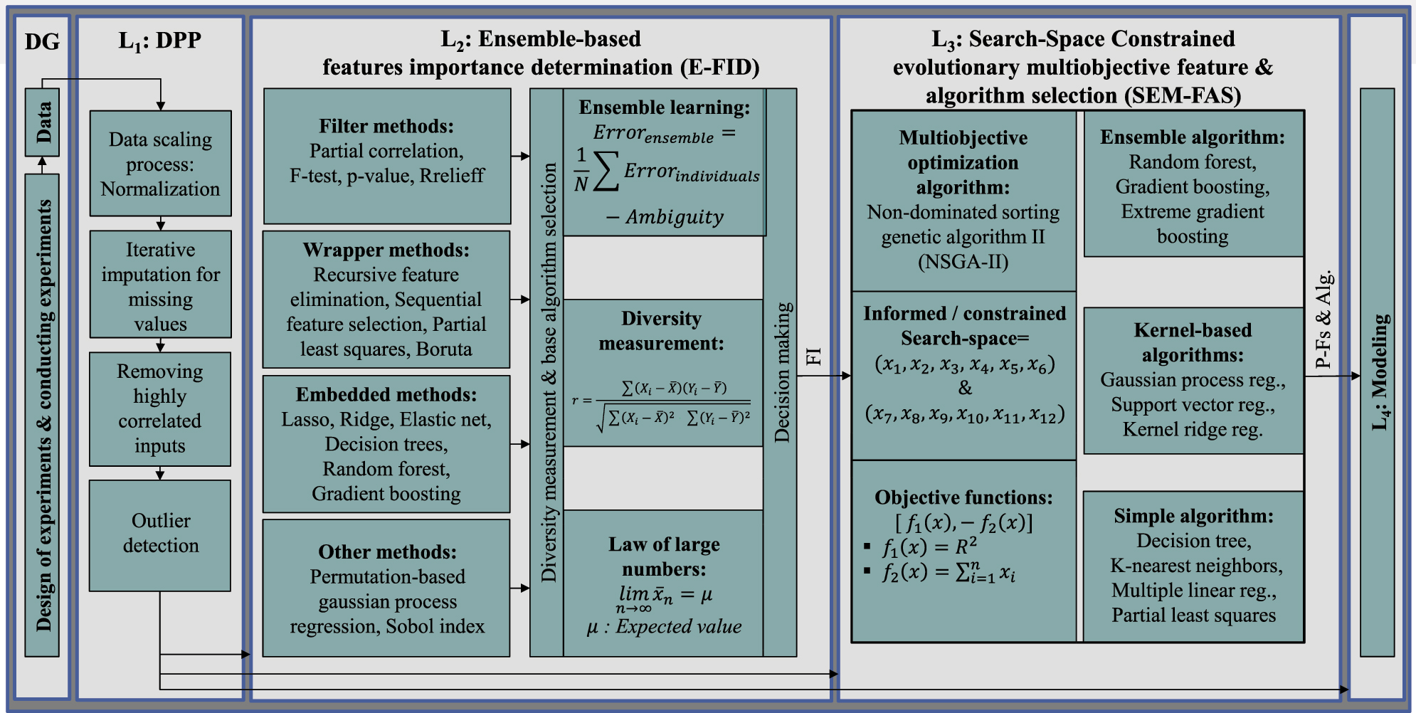
Proposed modeling pipeline for the ultra-high performance concrete manufacturing process, from data generation to modeling. (DG: Data generation, L: Layer, DPP: Data preprocessing, FI: Feature importance, P-Fs & Alg.: Proposed features & algorithm).
3.1 Key factors and characteristics in the UHPC production process
To collect data for the UHPC dataset
The dataset used in this study
| Group | Factor name | Var. | Unit | Mean | Median | Std | Min | Max |
|---|---|---|---|---|---|---|---|---|
| Material quality | Material delivery batch time | DB | Class | – | – | – | 1 | 2 |
| Ingredient moisture | IM | % | 3.13 | 3.15 | 0.16 | 2.92 | 3.36 | |
| Ingredient/Water temperature | IT | °C | 24.20 | 25 | 9.05 | 10 | 40 | |
| Graphite | GRP | kg | 0.08 | 0.09 | 0.07 | 0 | 0.22 | |
| Particle size distributions & Measurement errors | Sand I | SAI | kg | 5.98 | 6 | 0.59 | 5.10 | 6.90 |
| Sand II | SAII | kg | 10.53 | 10.50 | 1.04 | 8.92 | 12.07 | |
| Filler I | FLI | kg | 6.00 | 6 | 0.59 | 5.10 | 6.90 | |
| Filler II | FLII | kg | 0.75 | 0.75 | 0.07 | 0.63 | 0.86 | |
| Superplasticizer | SPP | kg | 0.32 | 0.32 | 0.02 | 0.29 | 0.35 | |
| Mixing condition | Average power consumption | APW | kW | 1.04 | 1.06 | 0.19 | 0.36 | 1.40 |
| Fresh concrete properties | Fresh concrete temperature | FCT | °C | 26.77 | 27 | 3.43 | 17.6 | 33.30 |
| Electrical conductivity | EC | V | 4.615 | 4.611 | 0.029 | 4.541 | 4.745 | |
| Air content | AC | % | 1.62 | 1.50 | 0.77 | 0.40 | 7 | |
| Slump flow | SF | mm | 335.91 | 340 | 26.35 | 215 | 395 | |
| Funnel runtime | FR | s | 7.53 | 7 | 2.82 | 4 | 24.10 | |
| Curing conditions | Curing temperature day 1 | CT1 | °C | 24.60 | 20 | 9.72 | 10 | 40 |
| Curing class day 1 | CC1 | Class | – | – | – | 1 | 2 | |
| Curing temperature day 2–28 | CT28 | °C | 22.15 | 20 | 9.38 | 10 | 40 | |
| Curing class day 2–28 | CC28 | Class | – | – | – | 1 | 2 |
In the first stage, the effects of material quality, storage environment, and silica fume impurities are examined by varying delivery batch time (DB), cement reactivity (CR), ingredient moisture (IM), ingredient temperature (IT), and graphite content (GRP). Even materials supplied by the same manufacturer but at different times (labeled as DB1 or DB2) can exhibit subtle differences that affect the microstructure. Cement reactivity can be altered by changes in chemical composition and environmental factors during storage. Variations in moisture content may also impact UHPC quality. Additionally, raw materials stored outside can experience fluctuations in temperature and humidity. Consequently, the temperature of raw materials is artificially adjusted, and extra water is added to simulate humidity. A crucial characteristic of UHPC is its low water content; thus, impurities that absorb water (e.g. GRP content) can significantly affect workability and, ultimately, compressive strength.
The recipe formulation (e.g. ratios of aggregates, superplasticizer, and silica fume) is critical for UHPC strength and durability. Small measurement errors or variations in particle size distribution can lead to significant differences in final properties. Various fresh concrete properties – temperature (FCT), electrical conductivity (EC), air content (AC), slump flow (SF), and funnel runtime (FR) – serve as indicators of homogeneity, workability, and potential structural integrity. To capture real-world variability, different curing conditions are implemented in two phases [23]. During the first 24 h, the UHPC transitions from paste to a minimally hardened state. It is either stored in a humidity-controlled cabinet at 90 % relative humidity and 20 °C or covered with plastic film at 20–40 °C. After demolding at 24 h, the specimens are either maintained under plastic film at 20 °C or submerged in water at 20–40 °C until day 28.
3.2 Data preprocessing
The data preprocessing stage consists of four main steps (Figure 2). First, data are normalized to the range [0, 1]. Second, iterative imputation manages missing data, which constitutes approximately 4 % of the dataset [3]. Simple methods like mean or median imputation can produce biased estimates [38]. Iterative imputation [39], implemented via scikit-learn’s IterativeImputer [40], treats each feature with missing values as a function of other features in a sequential modeling process. Thirdly, Pearson’s correlation coefficient [41] is used to detect and remove highly correlated inputs, preventing multicollinearity. The correlation analysis, detailed in Section 4.1, leads to the removal of three inputs, further reducing the dimensionality of the dataset
from 19 to 16 [3]. Finally, based on expert analysis [3], the removal of 11 outliers yields a refined dataset
3.3 Ensemble-based feature importance determination
In this study, the ensemble-based feature importance determination (E-FID) framework [2] is employed to identify predefined features as prior knowledge for incorporation into the next step (see Figure 2). Unlike single-model approaches, the ensemble method combines insights from multiple predictive algorithms, mitigating bias and variance issues. This strategy is particularly advantageous in high-dimensional, limited-data settings, where ensembles enhance generalization and reduce the risk of overfitting [19], [42].
E-FID utilizes 16 different feature importance determination methods as base learners (BLs), ranging from filter and wrapper to embedded approaches, to provide diverse perspectives for data analysis. Diversity among the BLs is measured using Pearson’s correlation analysis; highly correlated BLs are removed to eliminate redundancies. Finally, an averaging aggregate method is applied to combine the outcomes into the final result [2].
3.4 Search-space constrained evolutionary multiobjective feature and algorithm selection framework
3.4.1 Non-dominated sorting genetic algorithm II
This study adopts the non-dominated sorting genetic algorithm II (NSGA-II) [7] for feature selection. Each individual is represented by a binary vector:
where n is the total number of features, and x i ∈ {0, 1} indicates the absence (0) or presence (1) of the i-th feature. The fitness of each individual is quantified by multiple objective functions (f(x)), typically aiming to balance maximizing predictive performance against minimizing the number of selected features.
NSGA-II uses two main variation operators:
Crossover: Combines segments of two parent chromosomes to generate offspring.
Mutation: Randomly flips bits in a chromosome with probability μ, further enhancing diversity.
In each generation, the parent population P t undergoes crossover and mutation to produce an offspring population Q t . Both populations are then merged into R t and sorted by non-dominance and crowding distance to form the next generation [7].
The set of optimal solutions X * is defined by:
where l is the number of objectives, X is the set of all feasible solutions, and f i are the objective functions to be maximized, depending on the problem setup [43].
3.4.2 Search-space constrained non-dominated sorting genetic algorithm II
To address the challenges of EMOFS methods in high-dimensional datasets with small sizes, this study developed the search-space constrained non-dominated sorting genetic algorithm II (NSGA-II), as shown in Figure 3. The search-space constrained NSGA-II serves as an optimization process that selects the optimal features (i.e., dimensionality reduction) for modeling while simultaneously optimizing the hyperparameters of the chosen model. In the search-space constrained NSGA-II, an individual is represented by a vector.
where each x
i
∈ {0, 1} indicates whether the i-th feature is absent (0) or present (1), and each
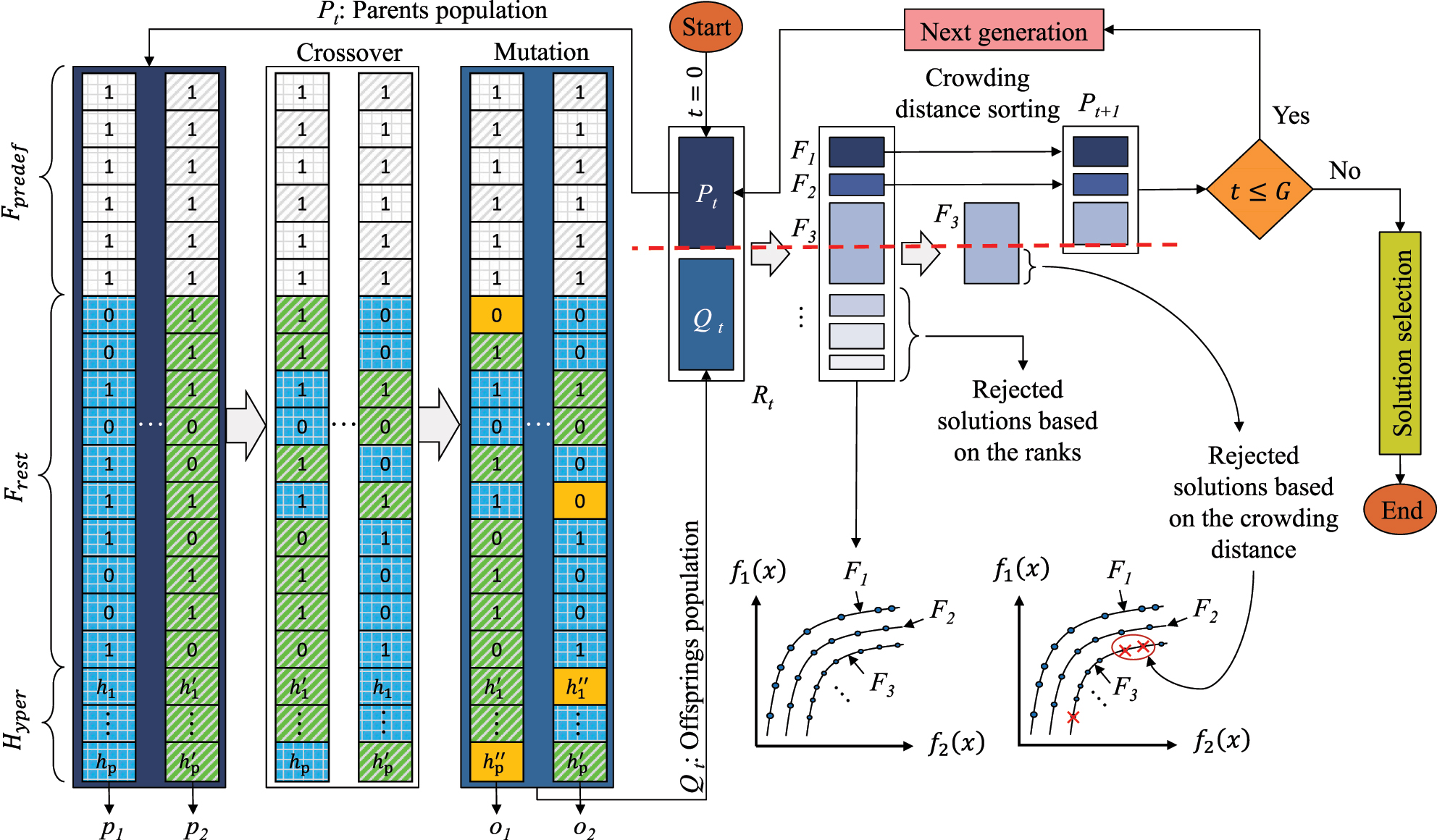
Overview of the search-space constrained NSGA-II process. Each generation selects parents (p c ) from the current population (P t ) for crossover and mutation, producing offspring (o c ) in (Q t ). After G generations, the final solutions comprise the predefined feature set (F predef), the non-predefined feature set (F rest), and the optimal hyperparameters (H yper). By enforcing features in (F predef) to be 1, NSGA-II narrows the search space, focusing on how other features (F rest) interact with F predef. (f i (x): Objective function, F i : Pareto solution).
Let S ⊆{1, 2, …, d} be the set of indices corresponding to these predefined features. During population initialization, crossover, and mutation, for each predefined feature index i ∈ S is enforced by setting x
i
= 1 (Figure 3). In the initialization phase, a population P
t
is created, each retaining the predefined feature set
During initialization, each individual has its predefined feature bits set to 1. For features not in the predefined set, bits are randomly chosen (0 or 1 with equal probability):
In the crossover step, two parents exchange bits for non-predefined features with probability α = 0.5. However, predefined feature bits (i ∈ S) are never swapped, so they remain 1 in each offspring (Figure 3).
In the mutation step, predefined feature bits are never flipped. For non-predefined features, each bit can flip with a small probability (μ = 0.05):
A uniform re-sampling mutation is applied to the hyperparameter genes: each hyperparameter is given an independent 5 % probability of being mutated, and, when mutation occurs, a new random value is drawn across its full valid range (a continuous uniform distribution for the real-valued and discrete uniform distributions for integer hyperparameters). In this way, each mutated value is kept admissible, fresh genetic material is injected at each generation, and the real-valued parameters are allowed to evolve jointly with the feature subset [45].
The fitness of each individual is evaluated as follows [43], [46]:
where f
1(x) = R
2(x) represents the model’s predictive accuracy, and
An alternative strategy to the proposed population initialization methodology is to integrate the predefined features directly into the fitness function – first applying NSGA-II only on non-predefined features and then combining them with the predefined ones – but this approach incurs extra computational overhead due to the repeated concatenation and separation of features. In contrast, the search-space constrained NSGA-II incorporates the predefined features from the initialization stage, ensuring they remain fixed during crossover and mutation for a more straightforward and efficient implementation.
3.4.3 Parameter settings and evaluation framework
In this study, both the search-space constrained and standard NSGA-II algorithms are implemented as sequential, single-threaded processes. The overall crossover probability is set to 0.7, meaning that 70 % of selected parent pairs undergo recombination. Within each crossover event, a gene-level probability of 0.5 is applied to swap features between individuals. Similarly, mutation is executed with an overall probability of 0.3, whereby each eligible gene has a 0.05 chance of being flipped.
In a nested modeling, validation, and evaluation loop, one test data point is held out at the start of the SEM-FAS framework using LOOCV for the final evaluation phase. Then, 10-fold cross-validation is performed on the remaining training data to train and validate each algorithm, thereby identifying the best features and hyperparameters for the chosen model via the search-space constrained NSGA-II. After finalizing the model and its optimal settings, the unseen test point is used for evaluation. These steps are repeated across multiple LOOCV folds, each with a different initialization, and the average prediction performance and frequency of feature selection are recorded. This entire procedure is then repeated for all 10 machine learning algorithms.
Considering the two objectives – prediction accuracy and feature count – the final solution selected from the Pareto front is the one that uses no more than 12 features while achieving the highest accuracy, as illustrated in Figure 4.
![Figure 4:
An illustration of the final solution selection strategy from a Pareto front for a maximization – minimization problem [47]. The chosen solution is the one that does not exceed 12 features while achieving the highest accuracy. (f
i
(x): Objective function).](/document/doi/10.1515/auto-2025-0025/asset/graphic/j_auto-2025-0025_fig_004.jpg)
An illustration of the final solution selection strategy from a Pareto front for a maximization – minimization problem [47]. The chosen solution is the one that does not exceed 12 features while achieving the highest accuracy. (f i (x): Objective function).
3.4.4 Machine learning algorithms
Within the SEM-FAS framework, the feature selection procedure employs a diverse set of 10 machine learning algorithms encompassing parametric and non-parametric methods, as well as linear, ensemble, and Bayesian approaches. The specific algorithms utilized are: multiple linear regression (MLR) [40], partial least squares (PLS) [40], [48], kernel ridge regression (KRR) [40], [49], k-nearest neighbors (KNN) [40], [50], support vector regression (SVR) [40], [51], decision tree (DT) [40], [51], random forest (RF) [40], [52], gradient boosting (GB) [40], [53], extreme gradient boosting (XGB) [54], and Gaussian process regression (GPR) [40], [55]. These algorithms are commonly applied in industrial prediction tasks [56], also for modeling the mechanical properties of concrete [57].
3.5 UHPC manufacturing process modeling
In the final layer of the proposed pipeline, the ranked features and the best-performing model (including optimal hyperparameters) identified by the SEM-FAS framework are employed (see Figure 2). This final stage implements a cumulative LOOCV procedure, in which features are cumulatively added to the previous feature subset in order of their importance, allowing an iterative assessment of how each additional feature and its interaction with others contribute to the final model’s performance (Alg. 1).
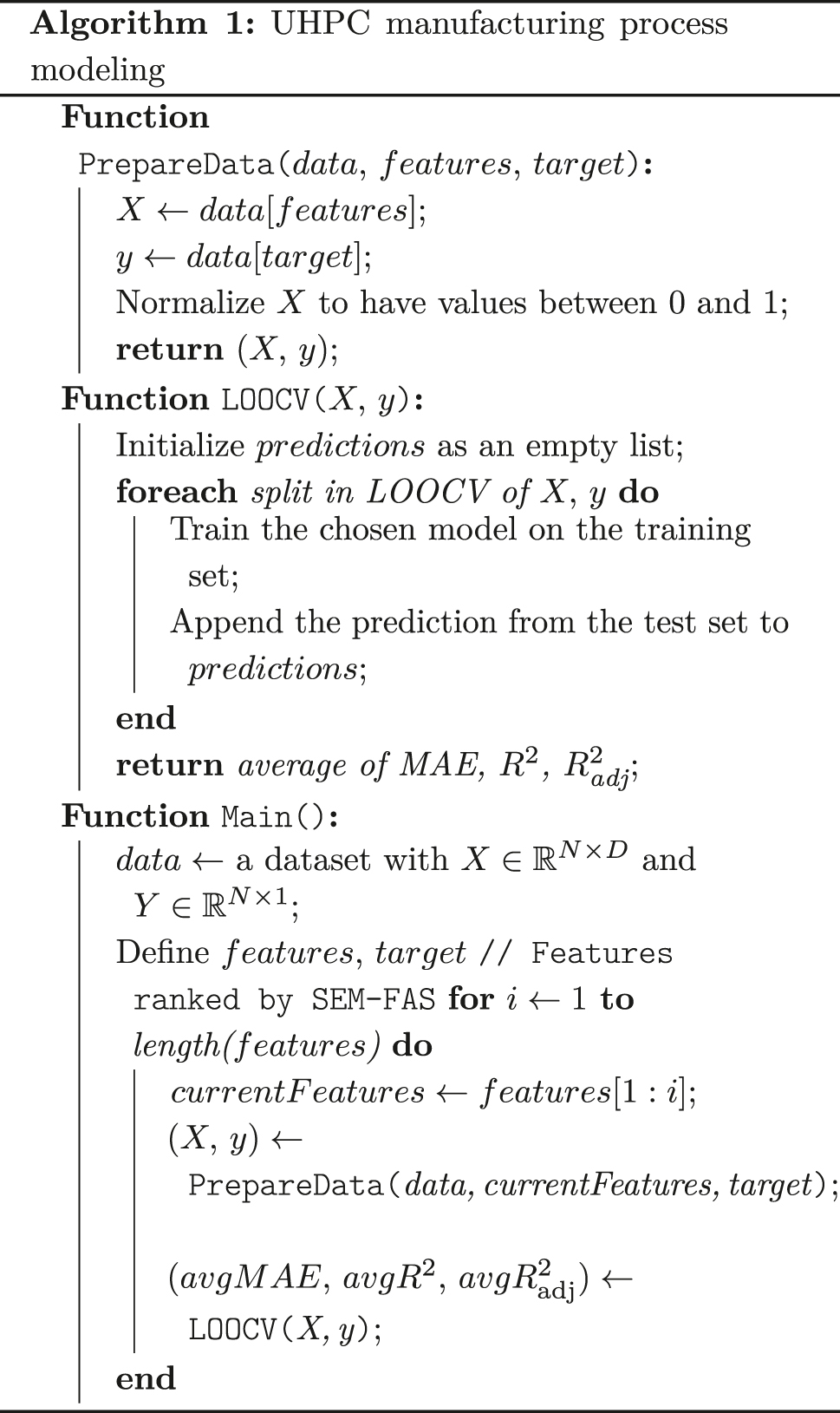 |
The cumulative LOOCV procedure systematically evaluates the incremental contribution of each feature based on its predefined ranking (from most important to least important), continuing until all features have been evaluated. The process is intentionally continued even if performance degrades at intermediate steps, because the goal is to provide comprehensive insights into the influence of each feature. The optimal number of features is thus clearly indicated by the resulting performance trajectory. Moreover, because each feature is evaluated in combination with all previously added features, interaction effects are implicitly captured and reflected in the predictive performance at each step.
4 Results and discussion
4.1 Correlation patterns in studied factors
The correlation analysis, presented in the heatmap in Figure 5, reveals strong linear correlations in specific variable pairs: SAI and SAII, FLI and FLII, and IT and FCT. Due to these high correlations, SAII, FLII, and FCT are removed, reducing the factor pool from 19 to 16 dimensions.
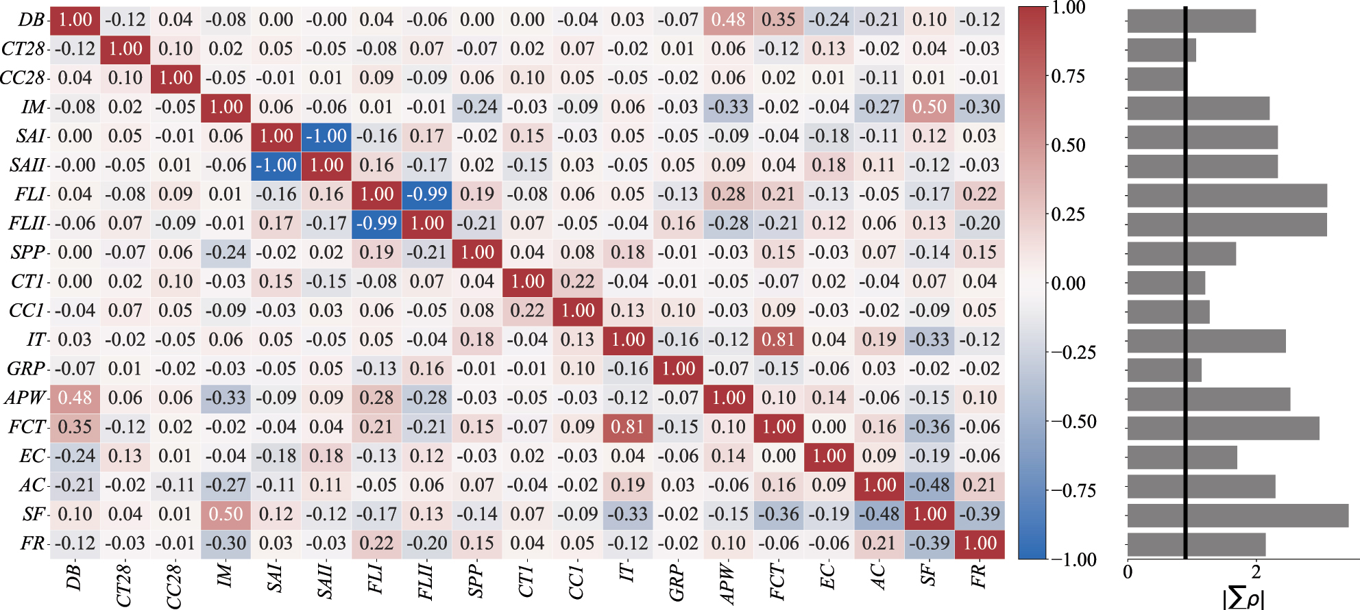
The Pearson correlation matrix of the 16 candidate input variables with a companion bar that displays the redundancy index
4.2 Gaining insights into feature importance for UHPC mechanical properties using E-FID
The feature importance analysis for CS28 (Figure 6) underscores the pivotal role of CT28, emphasizing the influence of environmental conditions during the second curing phase. Interestingly, CT1 on the first day of curing also emerges as significant, albeit less impactful than CT28. This finding suggests that conditions on the first day establish foundational strength, which is then further enhanced between days 2 and 28. It also reinforces the well-known principle that higher temperatures accelerate cement hydration, although ensuring adequate moisture in such environments remains vital.
![Figure 6:
Feature importance for compressive strength
(CS28) and flexural strength (FS28) at day 28. The figure highlights the dominance of curing temperatures and the varied impacts of material and environmental factors on these strengths. Feature relevances shown here are computed using the ensemble-based feature importance determination (E-FID) framework [2] by the aggregate averaging method described in Section 3.3. For definitions of the variables, refer to Table 1.](/document/doi/10.1515/auto-2025-0025/asset/graphic/j_auto-2025-0025_fig_006.jpg)
Feature importance for compressive strength (CS28) and flexural strength (FS28) at day 28. The figure highlights the dominance of curing temperatures and the varied impacts of material and environmental factors on these strengths. Feature relevances shown here are computed using the ensemble-based feature importance determination (E-FID) framework [2] by the aggregate averaging method described in Section 3.3. For definitions of the variables, refer to Table 1.
IM exerts a critical influence on final compressive strength, highlighting the importance of raw material moisture content. Likewise, while APW is not directly controllable, it serves as an informative indicator of energy input during mixing – reflecting UHPC paste rheology – and thus aids in predicting final compressive strength. Additionally, GRP and CC28 play notable roles. The presence of graphite (as an impurity in silica fume) can significantly absorb water in the mixture – an especially critical factor in UHPC given its low water content.
For FS28, as shown in Figure 6, CT28 remains paramount, reinforcing the overall impact of curing conditions. However, in a notable departure from compressive strength findings, CC28 emerges as the second most critical factor for flexural strength. This distinction underlines how environmental conditions influence the material’s resistance to bending stress.
IM and CT1 retain their importance across both compressive and flexural strengths, again emphasizing the role of moisture content and early-age curing. Notably, AC provides more predictive value for FS28 than for CS28, likely due to its effect on pore structure and distribution, which is especially relevant for flexural properties.
Based on these insights, the most important features are identified to form predefined feature vectors, serving as prior knowledge for the SEM-FAS framework. For CS28, the predefined features are CT28, CT1, IM, APW, GRP, and CC28. For FS28, the selected features are CT28, CC28, IM, CT1, AC, and DB.
4.3 Enhanced predictive modeling of UHPC mechanical properties by constraining the search-space of NSGA-II
4.3.1 Impact on model performance and algorithm selection
This study provides a comprehensive evaluation of 10 machine learning algorithms for predicting UHPC’s CS28 and FS28. In the SEM-FAS framework, each algorithm is trained and tested via LOOCV, with different random initializations in each fold. The modeling evaluates informed feature selection (I-FS) with search-space constrained NSGA-II, traditional feature selection (T-FS) with standard NSGA-II, and all features (ALL) for both mechanical properties. After training, each model’s performance is evaluated on unseen data using R 2 and MAE. The average results from all folds in the LOOCV loop (evaluation step) are summarized in Table 2. Models that use I-FS exhibit substantial improvements in R 2. For example, MLR’s R 2 increases from 72.47 % with T-FS to 76.21 % under I-FS. Moreover, reductions in MAE further validate the efficacy of I-FS. Notably, KRR’s R 2 rises from 62.38 % to 76.23 %, one of the largest observed improvements. For flexural strength (FS28), SVR shows the most significant gains. Its R 2 increases substantially, from 72.62 % under T-FS to 81.75 % under I-FS, indicating an enhanced capacity to capture flexural strength variability. The MAE also drops sharply, from 1.56 MPa to 0.93 MPa, reflecting more accurate predictions. GPR experiences a similar performance boost, with its R 2 rising from 72.67 % to 81.70 %, along with notable reductions in MAE.
Comparative analysis of modeling performance for compressive strength after 28 days (CS28) and flexural strength after 28 days (FS28) with informed feature selection (I-FS) using the search-space constrained NSGA-II, traditional feature selection (T-FS) using standard NSGA-II, and all features (ALL). For every model, I-FS yields higher predictive performance than T-FS (underfitting) and the full 16-feature model (overfitting), confirming that the proposed feature-aware evolutionary search balances parsimony and generalization more effectively than either extreme. Boldface marks the model selected for the final UHPC analysis for each mechanical property (Reg.: Regression, Ex.: Extreme) .
| Model | Abb. | CS28 | FS28 | ||||||||||
|---|---|---|---|---|---|---|---|---|---|---|---|---|---|
| R 2 in % | MAE in MPa | R 2 in % | MAE in MPa | ||||||||||
| I-FS | T-FS | All | I-FS | T-FS | All | I-FS | T-FS | All | I-FS | T-FS | All | ||
| Multiple linear reg | MLR | 76.21 | 72.47 | 72.50 | 4.66 | 5.26 | 5.03 | 78.06 | 74.02 | 74.17 | 1.15 | 1.53 | 1.42 |
| Partial least squares | PLS | 75.59 | 71.35 | 72.66 | 4.71 | 5.37 | 5.02 | 78.29 | 72.49 | 72.52 | 1.14 | 1.67 | 1.47 |
| Kernel ridge reg | KRR | 76.23 | 62.38 | 72.01 | 4.54 | 6.00 | 4.99 | 78.33 | 73.10 | 75.43 | 1.07 | 1.63 | 1.35 |
| K-nearest neighbors | KNN | 70.61 | 63.25 | 45.71 | 5.28 | 5.91 | 7.01 | 76.66 | 73.00 | 52.42 | 1.22 | 1.56 | 1.99 |
| Support vector reg | SVR | 73.18 | 68.93 | 69.48 | 5.05 | 5.54 | 5.48 | 81.75 | 72.62 | 76.19 | 0.93 | 1.56 | 1.24 |
| Decision tree | DT | 60.21 | 55.34 | 58.97 | 5.88 | 6.50 | 6.05 | 75.60 | 71.08 | 70.53 | 1.18 | 1.66 | 1.52 |
| Random forest | RF | 72.21 | 64.98 | 66.08 | 5.01 | 5.94 | 5.49 | 78.80 | 71.77 | 75.32 | 1.09 | 1.67 | 1.25 |
| Gradient boosting | GB | 71.53 | 60.77 | 66.66 | 5.01 | 6.00 | 5.50 | 77.10 | 72.26 | 74.93 | 1.05 | 1.60 | 1.30 |
| Ex. gradient boosting | XGB | 73.76 | 65.77 | 67.03 | 4.76 | 5.70 | 5.36 | 79.46 | 70.36 | 74.76 | 1.05 | 1.59 | 1.28 |
| Gaussian process reg | GPR | 75.36 | 67.47 | 68.06 | 4.76 | 5.73 | 5.01 | 81.70 | 72.67 | 75.82 | 0.96 | 1.57 | 1.20 |
In summary, applying I-FS consistently outperforms T-FS across all assessed metrics for both CS28 and FS28 (Table 2). The full-feature (ALL) model typically performs better than T-FS but worse than I-FS, confirming its tendency toward overfitting due to redundant information and highlighting the optimal balance provided by I-FS. The comparison of T-FS with ALL demonstrates the difficulty of feature selection in sparse datasets even with standard NSGA-II (T-FS), as its use based on these results often leads to the removal of important features, resulting in underfitting. These results confirm the superior predictive capabilities of the search-space constrained NSGA-II, particularly under the constraints of high dimensionality and small-sized data, where standard NSGA-II falters.
For CS28, MLR emerges as the best-performing model under I-FS, whereas for FS28, SVR achieves the highest accuracy. Consequently, these two models are selected for the final UHPC manufacturing process modeling.
4.3.2 Impact on solution stability and interpretability in the FS process
From Table 2, it is evident that models trained with search-space constrained NSGA-II can achieve higher predictive performance than those using standard NSGA-II. In this section, we examine how population initialization by injecting predefined features into NSGA-II affects solution stability and interpretability in the feature selection process for CS28 and FS28 (Figure 7). Figure 7 presents four heatmaps: for each mechanical property, one using I-FS and one using T-FS . In both scenarios, 139 runs are performed in a LOOCV train-test configuration across 10 models, and feature selection frequencies are recorded for each model.
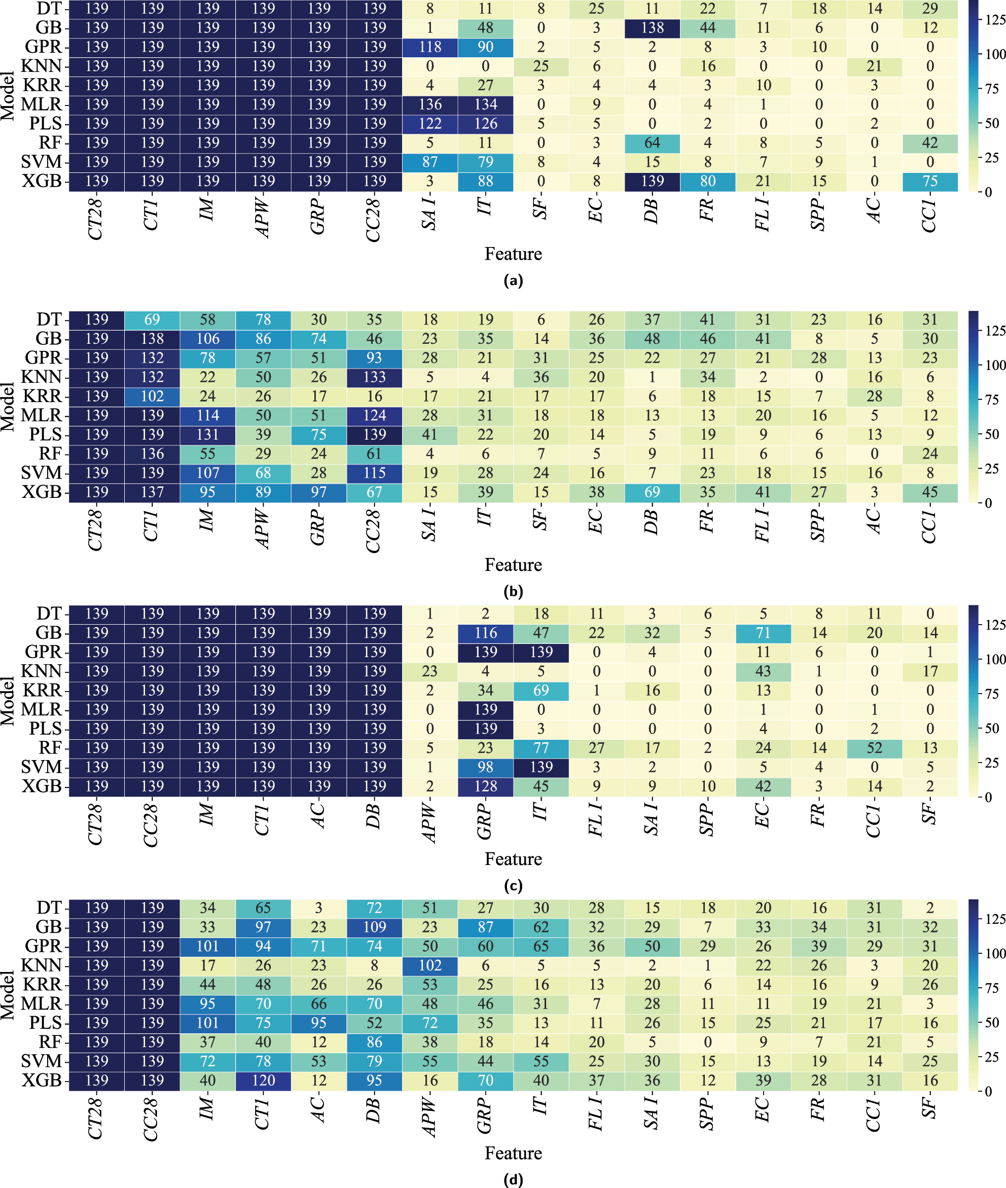
A comparative analysis of feature selection frequencies across the 16 candidate variables in I-FS and T-FS when predicting compressive and flexural strength at 28 days (CS28 and FS28) is presented. For each LOOCV fold, the feature subset on the Pareto front that achieves the highest predictive accuracy while using no more than 12 variables is selected. This yields final solutions whose number of selected features ranges from 6 to 12 under I-FS and from 1 to 12 under T-FS. See Table 1 for variable definitions. (a) Heatmap illustrating the frequency of feature selection in models employing I-FS for CS28. Under I-FS, models achieve greater solution stability and interpretability. (b) Heatmap displaying the frequency of feature selection in models using T-FS for CS28, showing higher variability in selected features. (c) Heatmap illustrating the frequency of feature selection using I-FS across all models for FS28, showing greater stability and interpretability. (d) Heatmap displaying the frequency of feature selection using T-FS for FS28, highlighting greater variability without domain-specific guidance.
Figure 7a (I-FS for CS28) shows that the six features predefined as the most critical are consistently chosen (139 times) across all models. In contrast, the T-FS scenario (Figure 7b), without predefined feature guidance, still identifies the same six features as most frequently selected, but with lower overall selection frequency. This consistency underscores the accuracy of the initial feature importance assessment by the E-FID method.
A notable difference between I-FS and T-FS lies in the stability of feature selection. I-FS consistently selects the predefined features in each model iteration, signifying enhanced stability, interpretability, and reliability in the selection process. By contrast, T-FS demonstrates higher selection variability, indicating potential instability in model performance without the injection of prior knowledge.
Additionally, features such as SAI, IT, and DB show substantially higher selection frequencies under I-FS, suggesting that the algorithm not only reinforces predefined features but also identifies and promotes other relevant factors based on intrinsic data characteristics. Conversely, features like SPP and CC1, which appear infrequently or not at all under I-FS, illustrate the capacity of I-FS to deprioritize less impactful features. This selective refinement by I-FS enhances both model interpretability and simplicity by clearly indicating which features provide consistent value for predicting CS28, while simultaneously ensuring stable solutions.
For FS28, Figure 7c shows that the predefined features CT28, CC28, IM, CT1, AC, and DB are each selected 139 times under I-FS. In contrast, the T-FS scenario (Figure 7d) displays more variability in feature selection. While features such as IM, CT1, AC, and DB remain frequently chosen, they appear with lower frequency than in the I-FS case. Moreover, I-FS reveals that APW, although significant under T-FS, is emphasized less when evaluated alongside the predefined features. Conversely, GRP and particularly EC, which T-FS deems less important, exhibit stronger interactions with predefined features under I-FS.
A broader comparison of feature selection frequencies (Figure 7) for both CS28 and FS28 shows that I-FS often assigns a frequency of zero to certain features, resulting in a clearer distinction between selected and non-selected features. This leads to more stable solutions, higher predictive accuracy, and improved interpretability.
As discussed in Section 4.3.1, MLR is the chosen algorithm for CS28 under I-FS, while SVR is selected for FS28. As shown in Figure 7a, the MLR model consistently selects CT28, CT1, IM, APW, GRP, CC28, SAI, IT, EC, FR, and FLI as the most critical features. Likewise, as shown in Figure 7c, the SVR model prioritizes CT28, CT1, IM, APW, GRP, CC28, SAI, IT, DB, SPP, SF, FR, FLI, and EC, reflecting their pivotal roles in the subsequent analysis phase.
4.4 Assessment of UHPC manufacturing process modeling
The results of the final modeling and evaluation of the selected models on unseen data are shown in Figure 8. The modeling process (Algorithm 1) for CS28 uses MLR and begins by adding the most influential factor, CT28 (Figure 8a). Using CT28 as a single predictor yields an R
2 value of 57.10 %, underscoring the predominant role of this curing temperature in explaining CS28 variance. Next, incorporating CT1 (the first 24 h of curing temperature) significantly enhances model performance, increasing R
2 to 66.61 %. This improvement suggests that CT1 provides additional variance information not captured by CT28. Adding IM raises R
2 to 70.53 %, and introducing APW increases it further to 71.16 %. Subsequently, including GRP and CC28 refines the model, lifting R
2 to 75.40 %. Although additional features such as SAI and IT only marginally increase R
2 to 75.77 %, they are retained based on domain expertise, reflecting their potential practical importance. Ultimately, the model achieves its highest
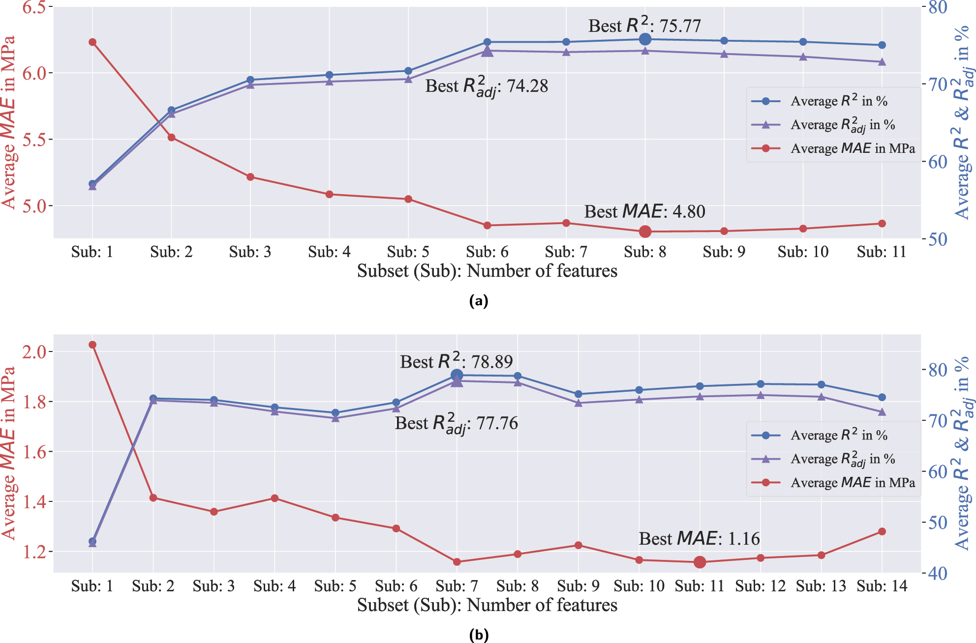
Comparative performance evaluation of MLR (multiple linear regression) and SVR (support vector regression) in the test phase. This figure shows how adding features affects the prediction metrics for CS28 and FS28. For CS28, Sub8 comprises CT28, CT1, IM, APW, GRP, CC28, SAI, and IT. For FS28, Sub7 includes CT28, CC28, IM, CT1, AC, DB, and IT. Variable definitions are in Table 1. (a) Prediction performance of MLR for CS28: Average R
2,
For FS28 modeling with SVR (Figure 8b), starting with CT28 alone yields an average R 2 of 46.23 %. Adding CC28 significantly enhances performance (to 74.32 %), underlining the importance of the curing conditions from day 2 to day 28. Incorporating additional variables such as IM, CT1, and AC leads to fluctuations in model accuracy; for instance, IM slightly lowers R 2 to 74.02 %, and CT1 plus AC reduce it further to 71.51 %. These variations suggest that while some factors add valuable information, others can introduce complexity without significantly improving predictive power. The model achieves its highest average R 2 of 78.89 % by also including DB and IT.
These findings (Figure 8) emphasize the critical role of curing conditions in optimizing the mechanical properties of UHPC. Additionally, factors related to material storage and delivery, which affect temperature and moisture content, significantly influence overall UHPC quality. Measurement errors in dosing key materials such as sand, along with impurities in silica fume (simulated as graphite content), substantially impact UHPC performance. These results illustrate why, in real-world scenarios, achieving the same final UHPC quality – even with an identical recipe – can be challenging if raw material storage conditions, silica fume impurities, dosing errors, and curing conditions (e.g., seasonal effects) are not properly managed.
5 Conclusions and future work
This study addresses a fundamental challenge in UHPC manufacturing: understanding why final UHPC quality can vary considerably even when an identical recipe is employed. By focusing on a single reference recipe and comprehensively investigating all relevant parameters – raw material storage conditions, possible measurement inaccuracies, mixing variables, and curing environments – this work provides a holistic perspective on the causal factors leading to inconsistencies in UHPC properties.
Considering the available high-dimensional but small-sized UHPC dataset [3], this study proposes a population-initialization method for multiobjective feature selection using NSGA-II to tackle dataset sparsity while investigating the relation between input features and the mechanical properties of UHPC. The proposed methodology outperforms the standard NSGA-II by achieving higher accuracy in predicting both compressive and flexural strength while offering more stable, interpretable, and reliable feature subsets.
The results of the modeling reveal why UHPC mixtures may fail to match prior performance levels despite following the same recipe. Poorly managed conditions – ranging from material temperature and moisture content to dosing errors, impurities in silica fume, and final curing – can introduce variations that significantly affect mechanical properties even when following the same recipe. These findings indicate that a sole reliance on a reference recipe is insufficient to reproduce the desired quality of the final UHPC product. By identifying and controlling the variables highlighted in this study, practitioners can move closer to replicating UHPC quality consistently in real-world scenarios.
Nevertheless, the scope of this research was confined to compressive and flexural strength of UHPC based on laboratory data. Future investigations should broaden these findings to additional mechanical properties, validate the proposed pipeline on other concrete classes – such as recycled concrete – and evaluate it in less controlled environments to better reflect real-world conditions.
Funding source: LOEWE – Landes-Offensive zur Entwicklung Wissenschaftlich-ökonomischer Exzellenz, Förderlinie 3: KMU-Verbundvorhaben (State Offensive for the Development of Scientific and Economic Excellence)
Award Identifier / Grant number: HA project no. 1650/23-203
About the authors

Farzad Rezazadeh, M.Sc., is a research assistant in the Department of Measurement and Control Engineering at the University of Kassel. His research focuses on data-driven modeling and machine learning.

Amin Abrishambaf, PhD., is a project manager in QuantumFusion GmbH. His expertise includes concrete technology, ultra high performance concrete and fiber reinforced concrete.

Prof. Dr.-Ing. Gregor Zimmermann is founder and head of MAITERIA, an AI driven platform for concrete materials and concrete optimization. Main research interests: ML driven concrete development and optimization, raw-material analysis and digitization, concrete DNA development.

Univ.-Prof. Dr.-Ing. Andreas Kroll is head of the Department of Measurement and Control Engineering at the University of Kassel. Main research interests: Nonlinear system identification and control methods; computational intelligence; remote sensing and sensor data fusion.
-
Research ethics: Not applicable.
-
Informed consent: Not applicable.
-
Author contributions: Farzad Rezazadeh: writing – original draft, conceptualization, data curation, formal analysis, methodology, software, validation, visualization. Amin Abrishambaf: conceptualization, validation, writing – review and editing. Gregor Zimmermann: conceptualization, funding acquisition, project administration, resources. Andreas Kroll: conceptualization, funding acquisition, project administration, resources, supervision, writing – review and editing.
-
Use of Large Language Models, AI and Machine Learning Tools: None declared.
-
Conflict of interest: The author states no conflict of interest.
-
Research funding: This project (HA project no. 1650/23-203) is financed with funds of LOEWE – Landes-Offensive zur Entwicklung Wissenschaftlich-ökonomischer Exzellenz, Förderlinie 3: KMU-Verbundvorhaben (State Offensive for the Development of Scientific and Economic Excellence).
-
Data availability: The datasets analyzed during the current study are available in the DaKS – University of Kassel's research data repository, https://doi.org/10.48662/daks-56.
-
Software availability: The underlying code and related data are available upon reasonable request from the corresponding author.
References
[1] A. Abrishambaf, M. Pimentel, S. Nunes, and C. Costa, “Multi-level study on UHPFRC incorporating ECat,” Constr. Build. Mater., vol. 318, p. 125976, 2022, https://doi.org/10.1016/j.conbuildmat.2021.125976.Search in Google Scholar
[2] F. Rezazadeh P, A. Dürrbaum, G. Zimmermann, and A. Kroll, “Leveraging ensemble structures to elucidate the impact of factors that influence the quality of ultra-high performance concrete,” in 2023 IEEE Symposium Series on Computational Intelligence (SSCI), Mexico City, IEEE, 2023, pp. 180–187.10.1109/SSCI52147.2023.10371800Search in Google Scholar
[3] F. Rezazadeh, A. Dürrbaum, A. Abrishambaf, G. Zimmermann, and A. Kroll, “Mechanical properties of ultra-high performance concrete (UHPC),” 2025, [Online]. Available: https://daks.uni-kassel.de/handle/123456789/251.Search in Google Scholar
[4] D. W. Aha and R. L. Bankert, “A comparative evaluation of sequential feature selection algorithms,” in Pre-proceedings of the Fifth International Workshop on Artificial Intelligence and Statistics, Fort Lauderdale, Florida, PMLR, 1995, pp. 1–7.Search in Google Scholar
[5] M. Amoozegar, and B. Minaei-Bidgoli, “Optimizing multi-objective PSO based feature selection method using a feature elitism mechanism,” Expert Syst. Appl., vol. 113, pp. 499–514, 2018, https://doi.org/10.1016/j.eswa.2018.07.013.Search in Google Scholar
[6] R. Jiao, B. H. Nguyen, B. Xue, and M. Zhang, “A survey on evolutionary multiobjective feature selection in classification: Approaches, applications, and challenges,” IEEE Trans. Evol. Comput., vol. 28, no. 4, pp. 1156–1176, 2024, https://doi.org/10.1109/tevc.2023.3292527.Search in Google Scholar
[7] K. Deb, A. Pratap, S. Agarwal, and T. Meyarivan, “A fast and elitist multiobjective genetic algorithm: NSGA-II,” IEEE Trans. Evol. Comput., vol. 6, no. 2, pp. 182–197, 2002, https://doi.org/10.1109/4235.996017.Search in Google Scholar
[8] S. Popovics, “Analysis of concrete strength versus water-cement ratio relationship,” ACI Mater. J., vol. 87, no. 5, pp. 517–529, 1990.10.14359/1944Search in Google Scholar
[9] E. M. Golafshani, A. Behnood, T. Kim, T. Ngo, and A. Kashani, “Metaheuristic optimization based-ensemble learners for the carbonation assessment of recycled aggregate concrete,” Appl. Soft Comput., vol. 159, p. 111661, 2024, https://doi.org/10.1016/j.asoc.2024.111661.Search in Google Scholar
[10] R. Kumar, B. Rai, and P. Samui, “A comparative study of prediction of compressive strength of ultra-high performance concrete using soft computing technique,” Struct. Concr., vol. 24, no. 4, pp. 5538–5555, 2023, https://doi.org/10.1002/suco.202200850.Search in Google Scholar
[11] I. C. Yeh, “Modeling of strength of high-performance concrete using artificial neural networks,” Cem. Concr. Res., vol. 28, no. 12, pp. 1797–1808, 1998, https://doi.org/10.1016/s0008-8846-98-00165-3.Search in Google Scholar
[12] I. C. Yeh, “Modeling slump flow of concrete using second-order regressions and artificial neural networks,” Cement Concr. Compos., vol. 29, no. 6, pp. 474–480, 2007, https://doi.org/10.1016/j.cemconcomp.2007.02.001.Search in Google Scholar
[13] M. H. Rafiei, et al.., “Neural network, machine learning, and evolutionary approaches for concrete material characterization,” ACI Mater. J., vol. 113, no. 6, pp. 781–789, 2016, https://doi.org/10.14359/51689360.Search in Google Scholar
[14] J. Yu, R. Pan, and Y. Zhao, “High-dimensional, small-sample product quality prediction method based on MIC-stacking ensemble learning,” Appl. Sci., vol. 12, no. 1, p. 23, 2022, https://doi.org/10.3390/app12010023.Search in Google Scholar
[15] N.-H. Nguyen, J. Abellán-García, S. Lee, E. Garcia-Castano, and T. P. Vo, “Efficient estimating compressive strength of ultra-high performance concrete using XGBoost model,” J. Build. Eng., vol. 52, p. 104302, 2022, https://doi.org/10.1016/j.jobe.2022.104302.Search in Google Scholar
[16] B. K. Aylas-Paredes, et al.., “Data driven design of ultra high performance concrete prospects and application,” Sci. Rep., vol. 15, no. 1, 2025, Art. no. 9248, [Online]. Available: https://doi.org/10.1038/s41598-025-94484-2.Search in Google Scholar PubMed PubMed Central
[17] T. G. Wakjira, A. A. Kutty, and M. S. Alam, “A novel framework for developing environmentally sustainable and cost-effective ultra-high-performance concrete (UHPC) using advanced machine learning and multi-objective optimization techniques,” Constr. Build. Mater., vol. 416, p. 135114, 2024. [Online]. Available: https://doi.org/10.1016/j.conbuildmat.2024.135114.Search in Google Scholar
[18] J. Abellán-García, “Study of nonlinear relationships between dosage mixture design and the compressive strength of UHPC,” Case Stud. Constr. Mater., vol. 17, p. e01228, 2022, [Online]. Available: https://doi.org/10.1016/j.cscm.2022.e01228.Search in Google Scholar
[19] F. Rezazadeh, E. Olfatbakhsh, and A. Kroll, “Sign diversity: A method for measuring diversity in base learner selection for ensemble regression,” in Proceedings of the 2025 IEEE Symposium on Computational Intelligence on Engineering/Cyber Physical Systems (CIES), Trondheim, IEEE, 2025, pp. 1–9.10.1109/CIES64955.2025.11007635Search in Google Scholar
[20] S. Mahjoubi, W. Meng, and Y. Bao, “Auto-tune learning framework for prediction of flowability, mechanical properties, and porosity of ultra-high-performance concrete (UHPC),” Appl. Soft Comput., vol. 115, p. 108182, 2022, https://doi.org/10.1016/j.asoc.2021.108182.Search in Google Scholar
[21] E. M. Golafshani, A. Behnood, T. Kim, T. Ngo, and A. Kashani, “A framework for low-carbon mix design of recycled aggregate concrete with supplementary cementitious materials using machine learning and optimization algorithms,” Struct., vol. 61, p. 106143, 2024. https://doi.org/10.1016/j.istruc.2024.106143.Search in Google Scholar
[22] Z. Li, et al.., “Machine learning in concrete science: Applications, challenges, and best practices,” npj Comput. Mater., vol. 8, no. 1, p. 127, 2022, https://doi.org/10.1038/s41524-022-00810-x.Search in Google Scholar
[23] F. Rezazadeh P, A. Dürrbaum, G. Zimmermann, and A. Kroll, “Holistic modeling of ultra-high performance concrete production process: synergizing mix design, fresh concrete properties, and curing conditions,”in Proceedings - 33. Workshop Computational Intelligence, Berlin, KIT Scientific Publishing, 2023, pp. 215–237. 23.-24. November 2023.10.58895/ksp/1000162754-15Search in Google Scholar
[24] P. Refaeilzadeh, L. Tang, and H. Liu, “Cross-validation,” in Proceedings of the Encyclopedia of Database Systems, Boston, Springer US, 2009, pp. 532–538.10.1007/978-0-387-39940-9_565Search in Google Scholar
[25] I. Vatolkin, M. Preuß, and G. Rudolph, “Multiobjective feature selection in music genre and style recognition tasks,” in Proceedings of the 13th annual conference on Genetic and evolutionary computation, Dublin, ACM, 2011, pp. 411–418.10.1145/2001576.2001633Search in Google Scholar
[26] B. Ahadzadeh, M. Abdar, F. Safara, A. Khosravi, M. B. Menhaj, and P. N. Suganthan, “SFE: A simple, fast, and efficient feature selection algorithm for high-dimensional data,” IEEE Trans. Evol. Comput., vol. 27, no. 6, pp. 1896–1911, https://doi.org/10.1109/tevc.2023.3238420, 2023.Search in Google Scholar
[27] L. Li, M. Xuan, Q. Lin, M. Jiang, Z. Ming, and K. C. Tan, “An evolutionary multitasking algorithm with multiple filtering for high-dimensional feature selection,” IEEE Trans. Evol. Comput., vol. 27, no. 4, pp. 802–816, 2023, https://doi.org/10.1109/tevc.2023.3254155.Search in Google Scholar
[28] K. Chen, B. Xue, M. Zhang, and F. Zhou, “Evolutionary multitasking for feature selection in high-dimensional classification via particle swarm optimization,” IEEE Trans. Evol. Comput., vol. 26, no. 3, pp. 446–460, 2022, https://doi.org/10.1109/tevc.2021.3100056.Search in Google Scholar
[29] J. Luo, D. Zhou, L. Jiang, and H. Ma, “A particle swarm optimization based multiobjective memetic algorithm for high-dimensional feature selection,” Memetic Comput., vol. 14, no. 1, pp. 77–93, 2022, https://doi.org/10.1007/s12293-022-00354-z.Search in Google Scholar
[30] L. Von Rueden, et al.., “Informed machine learning - a taxonomy and survey of integrating prior knowledge into learning systems,” IEEE Trans. Knowl. Data Eng., vol. 32, no. 1, pp. 614–633, 2023. https://doi.org/10.1109/tkde.2021.3079836.Search in Google Scholar
[31] I. Kropp, A. P. Nejadhashemi, and K. Deb, “Benefits of sparse population sampling in multi-objective evolutionary computing for large-scale sparse optimization problems,” Swarm Evol. Comput., vol. 69, p. 101025, 2022, https://doi.org/10.1016/j.swevo.2021.101025.Search in Google Scholar
[32] H. Xu, B. Xue, and M. Zhang, “A duplication analysis-based evolutionary algorithm for biobjective feature selection,” IEEE Trans. Evol. Comput., vol. 25, no. 2, pp. 205–218, 2021, https://doi.org/10.1109/tevc.2020.3016049.Search in Google Scholar
[33] X.-F. Song, Y. Zhang, D.-W. Gong, and X.-Z. Gao, “A fast hybrid feature selection based on correlation-guided clustering and particle swarm optimization for high-dimensional data,” IEEE Trans. Cybern., vol. 52, no. 9, pp. 9573–9586, 2022, https://doi.org/10.1109/tcyb.2021.3061152.Search in Google Scholar
[34] J. Ren, F. Qiu, and H. Hu, “Multiple sparse detection-based evolutionary algorithm for large-scale sparse multiobjective optimization problems,” Complex Intell. Syst., vol. 9, no. 4, pp. 4369–4388, 2023, https://doi.org/10.1007/s40747-022-00963-8.Search in Google Scholar
[35] P. Wang, B. Xue, J. Liang, and M. Zhang, “Multiobjective differential evolution for feature selection in classification,” IEEE Trans. Cybern., vol. 53, no. 7, pp. 4579–4593, 2023. [Online]. Available: https://doi.org/10.1109/tcyb.2021.3128540.Search in Google Scholar
[36] I. Vatolkin, G. Rudolph, and C. Weihs, Interpretability of Music Classification as a Criterion for Evolutionary multi-objective Feature Selection, Copenhagen, Springer International Publishing, 2015, pp. 236–248, [Online]. Available: https://doi.org/10.1007/978-3-319-16498-4_21.Search in Google Scholar
[37] A. Dürrbaum, F. Rezazadeh, and A. Kroll, “Automatic camera-based advanced slump flow testing for improved reliability,” in Proceedings of the 2023 IEEE SENSORS, Vienna, IEEE, 2023, pp. 1–4.10.1109/SENSORS56945.2023.10325030Search in Google Scholar
[38] A. R. T. Donders, G. J. van der Heijden, T. Stijnen, and K. G. Moons, “Review: A gentle introduction to imputation of missing values,” J. Clin. Epidemiol., vol. 59, no. 10, pp. 1087–1091, 2006.10.1016/j.jclinepi.2006.01.014Search in Google Scholar PubMed
[39] R. J. A. Little and D. B. Rubin, Statistical Analysis with Missing Data, 3rd ed. Hoboken, NJ, John Wiley & Sons, 2019.10.1002/9781119482260Search in Google Scholar
[40] F. Pedregosa, et al.., “Scikit-learn: Machine learning in Python,” J. Mach. Learn. Res., vol. 12, pp. 2825–2830, 2011.Search in Google Scholar
[41] J. Benesty, J. Chen, Y. Huang, and I. Cohen, “Pearson correlation coefficient,” in Noise Reduction in Speech Processing, vol. 2, Berlin, Heidelberg, Springer, 2009, pp. 1–4.10.1007/978-3-642-00296-0_5Search in Google Scholar
[42] O. Sagi, and L. Rokach, “Ensemble learning: A survey,” WIREs Data Min. Knowl. Discov., vol. 8, no. 4, p. e1249, 2018, https://doi.org/10.1002/widm.1249.Search in Google Scholar
[43] L. Wang, A. H. C. Ng, and K. Deb, “Multi-objective optimisation using evolutionary algorithms: An introduction,” in Multi-objective Evolutionary Optimisation for Product Design and Manufacturing, London, Springer, 2011, pp. 3–34.10.1007/978-0-85729-652-8_1Search in Google Scholar
[44] M. Binder, J. Moosbauer, J. Thomas, and B. Bischl, “Multi-objective hyperparameter tuning and feature selection using filter ensembles,” in Proceedings of the 2020 Genetic and Evolutionary Computation Conference, Cancún, ACM, 2020, pp. 471–479.10.1145/3377930.3389815Search in Google Scholar
[45] K. Deb, Multi-Objective Optimization Using Evolutionary Algorithms, New York, NY, John Wiley & Sons, 2001.Search in Google Scholar
[46] H. Ishibuchi, R. Imada, Y. Setoguchi, and Y. Nojima, “Hypervolume subset selection for triangular and inverted triangular pareto fronts of three-objective problems,” in Proceedings of the 14th ACM/SIGEVO Conference on Foundations of Genetic Algorithms, Copenhagen, ACM, 2017.10.1145/3040718.3040730Search in Google Scholar
[47] R. Khezri, and A. Mahmoudi, “Review on the state-of-the-art multi-objective optimisation of hybrid standalone/grid-connected energy systems,” IET Generat. Transm. Distrib., vol. 14, no. 20, pp. 4285–4300, 2020.10.1049/iet-gtd.2020.0453Search in Google Scholar
[48] J. A. Wegelin, A Survey of Partial Least Squares (PLS) Methods, with Emphasis on the Two-Block Case, Dept. of Statistics, University of Washington, Seattle, WA, Tech. Rep. 371, 2000.Search in Google Scholar
[49] K. P. Murphy, Machine Learning: A Probabilistic Perspective, Cambridge, MA, MIT Press, 2012.Search in Google Scholar
[50] E. Fix, and J. L. Hodges, “Discriminatory analysis. Nonparametric discrimination: Consistency properties,” Int. Stat. Rev/Revue Internationale de Statistique, vol. 57, no. 3, p. 238, 1989. [Online]. Available: https://doi.org/10.2307/1403797.Search in Google Scholar
[51] L. Hamel, Knowledge Discovery with Support Vector Machines, Hoboken, NJ, Wiley, 2009, [Online]. Available: https://doi.org/10.1002/9780470503065.Search in Google Scholar
[52] L. Breiman, “Random forests,” Mach. Learn., vol. 45, pp. 5–32, 2001. https://doi.org/10.1023/A:1010933404324.Search in Google Scholar
[53] J. H. Friedman, “Greedy function approximation: A gradient boosting machine,” Ann. Stat., vol. 29, no. 5, pp. 1189–1232, 2001, https://doi.org/10.1214/aos/1013203451.Search in Google Scholar
[54] T. Chen and C. Guestrin, “XGBoost: A scalable tree boosting system,” in Proceedings of the 22nd ACM SIGKDD International Conference on Knowledge Discovery and Data Mining, San Francisco, CA, ACM, 2016, pp. 785–794.10.1145/2939672.2939785Search in Google Scholar
[55] C. E. Rasmussen, “Gaussian processes in machine learning,” in Advanced Lectures on Machine Learning, vol. 3176, Berlin, Heidelberg, Springer, 2004, pp. 63–71.10.1007/978-3-540-28650-9_4Search in Google Scholar
[56] Z. Ge, Z. Song, S. X. Ding, and B. Huang, “Data mining and analytics in the process industry: The role of machine learning,” IEEE Access, vol. 5, pp. 20590–20616, 2017. https://doi.org/10.1109/access.2017.2756872.Search in Google Scholar
[57] F. Rezazadeh and A. Kroll, “Predicting the compressive strength of concrete up to 28 Days-ahead: Comparison of 16 machine learning algorithms on benchmark datasets,” in Proceedings - 32. Workshop Computational Intelligence, Berlin, KIT Scientific Publishing, 2022, pp. 53–75.10.58895/ksp/1000151141-4Search in Google Scholar
© 2025 the author(s), published by De Gruyter, Berlin/Boston
This work is licensed under the Creative Commons Attribution 4.0 International License.
Articles in the same Issue
- Frontmatter
- Editorial
- Selected contributions from the workshops “Computational Intelligence” in 2023 and 2024
- Methods
- Nonlinear system categorization for structural data mining with state space models
- Incorporation of structural properties of the response surface into oblique model trees
- Takagi-Sugeno based model reference control for wind turbine systems in frequency containment scenarios
- On autoregressive deep learning models for day-ahead wind power forecasts with irregular shutdowns due to redispatching
- Applications
- Efficiently determining the effect of data set size on autoencoder-based metamodels for structural design optimization
- Kalibriermodellerstellung und Merkmalsselektion für die mikromagnetische Materialcharakterisierung mittels maschineller Lernverfahren
- Investigating quality inconsistencies in the ultra-high performance concrete manufacturing process using a search-space constrained non-dominated sorting genetic algorithm II
- EAP4EMSIG – enhancing event-driven microscopy for microfluidic single-cell analysis