Existence of multiple nontrivial solutions of the nonlinear Schrödinger-Korteweg-de Vries type system

Qiuping Geng; Jun Wang; Jing Yang

doi:10.1515/anona-2021-0214

Article Open Access

Existence of multiple nontrivial solutions of the nonlinear Schrödinger-Korteweg-de Vries type system

Qiuping Geng , Jun Wang and Jing Yang

Published/Copyright: November 23, 2021

Published by

Become an author with De Gruyter Brill

Submit Manuscript Author Information Explore this Subject

From the journal Advances in Nonlinear Analysis Volume 11 Issue 1

Abstract

In this paper we are concerned with the existence, nonexistence and bifurcation of nontrivial solution of the nonlinear Schrödinger-Korteweg-de Vries type system(NLS-NLS-KdV). First, we find some conditions to guarantee the existence and nonexistence of positive solution of the system. Second, we study the asymptotic behavior of the positive ground state solution. Finally, we use the classical Crandall-Rabinowitz local bifurcation theory to get the nontrivial positive solution. To get these results we encounter some new challenges. By combining the Nehari manifolds constraint method and the delicate energy estimates, we overcome the difficulties and find the two bifurcation branches from one semitrivial solution. This is an new interesting phenomenon but which have not previously been found.

Keywords: Positive solutions; Bifurcation theory; Critical points; Nonlinear Schrödinger-Korteweg-de Vries system

MSC 2010: 35J61; 35J20; 35Q55; 49J40

1 Introduction and main results

1.1 Introduction

In this paper we study the following nonlinear Schrödinger-Korteweg-de Vries type system(NLS-NLS-KdV)

(1.1) −Δu+λ1u=μ1u3+β12uv2+β13uw,−Δv+λ2v=μ2v3+β12u2v+β23vw,−Δw+λ3w=μ3w2+12β13u2+12β23v2,

where u, v, wϵH¹(ℝ^N), N≥1, λi>0(i=1,2,3) , and β12>0 , μi(i=1,2,3),β13,β23∈R are constants. This kind of system has been applied in many physical models. For example, the [18] studied the following coupled nonlinear Schrödinger-Korteweg-de Vries (NLS-KdV for short) system

(1.2) ift+D2f=βfg−|f|2f,gt+D3g+gDg=β2D(|f|2),

where D=∂∂x , f=f(x,t)∈C , g=g(x,t)∈R , and β∈R is a coupling parameter. This type system appears in phenomena of interactions between short and long dispersive waves, arising in fluid mechanics, such as the interactions of capillary-gravity waves [28]. Indeed, f represents the short-wave, while g stands for the long-wave. One can refer to the papers [2, 9, 17,18,19,25,26] and the references therein for further details on similar system. Note that the interaction between long and short waves appear in magnetised plasma [27,51] and in many physical phenomena as well, such as Bose-Einstein condensates [12, 13, 41]. If we look for the solution of (1.2) in the following form

(f(x,t),g(x,t))=(eiωteikxu(x−ct),v(x−ct)),

which can be called solitary “standing-traveling”, then the system (1.2) leads to

−u′′+λ1u=u3+βuv,−v′′+λ2v=12v2+12βu2,

where N=1, λ₁=c^*:=k²+ω and λ₂=c=2k. The paper [18] studied the existence of positive bound and ground states of the system. Also, this system was studied by Dias et al. in [21], they studied this system in the particular case λ₁=λ₂ and they proved the existence of non-negative bound state solutions when the coupling parameter β>12 . The papers [18, 26, 33] considered the general dimensional case for the system

(1.3) −Δu+λ1u=u3+βuv,−Δv+λ2v=12v2+12βu2.

System (1.3) can be seen as the stationary system of two coupled NLS-NLS equations when one looks for solitary wave solutions. The systems of NLS-NLS time-dependent equations are used in some aspects of optics, Hartree-Fock theory for Bose-Einstein condensates, among other physical phenomena, see for example [1, 2,3,4,5, 7,14, 32, 42,43, 45] and references therein. In the dimensional case N=2, 3, the paper [33] proved a partial result on the existence of solutions to (1.3). The existence of a positive radially symmetric ground state of (1.3) in dimensional case N=1, 2, 3 were proved in [18]. The paper [26] made the complete study of the existence, bifurcation and asymptotic behavior of the positive solutions of (1.3) for N≥1 by combining the Nehari manifolds and Crandall-Rabinowitz local bifurcation theory. Also, see the paper [29] for the asymptotic expansion of the ground state energy for the nonlinear Schrödinger system with quadratic nonlinearity.

For the three coupled system (1.2), the paper [18, 26] generalized the system (1.3) to the nonlinear Schrödinger-Korteweg-de Vries-Korteweg-de Vries(NLS-KdV-KdV) system

(1.4) −Δu+λ1u=μ1|u|2u+β˜1uv+β˜2uw, in RN,−Δv+λ2v=μ2|v|v+12β˜1u2, in RN,−Δw+λ3w=μ3|w|w+12β˜2u2, in RN,

where u,v,w∈H1(RN),N≥1,λ1,λ2,λ3,μ1,μ2,μ3>0 and β˜1,β˜2∈R are constants. [18] proved the existence of radial bound state when β12,β13,β23>0 and positive radial ground state of (1.4) when the coupling parameters β₁₂, β₁₃, β₂₃ are sufficiently large. Multiple positive solutions of (1.4) are considered by a combination of Nehari manifold and bifurcation methods in [26].

Another motivation to study the system (1.2) is that it relates to the following parabolic system

(1.5) ∂u∂t−Δu=f1(x,u,v,w),(x,t)∈Ω×(T0,∞),∂v∂t−Δv=f2(x,u,v,w),(x,t)∈Ω×(T0,∞),∂w∂t−Δw=f3(x,u,v,w), (x,t)∈Ω×(T0,∞),

where Ω⊆ℝ^N is an open set. The system (1.4) has been recently studied in various mathematical directions. For example, the local and global existence [6,35], Höder regularity [20], symmetry property [24], blow-up behavior [34], and Liouville-type theorems [24,36, 37, 40]. If F⃗:=(f1,f2,f3)=(u3+β12uv2+β13uw−λ1u,v3+β12v2u+β23vw−λ2v,12w2+12β13u2+12β23v2−λ3w) , the paper [18] prove the existence of radial solution of the stationary solution of the system (1.4) for β_ij(i=1, 2; j=2, 3; i≠j) sufficiently small by using the perturbation methods. The authors [10] considered the existence and stability for solutions of the system (1.4) in the one dimension with β₁₂=0 and including other sub-critical nonlinearities. Here the stationary solution means that the solution does not dependent on the time t. If F⃗:=(f1,f2,f3)=(μ1|u|p−2u+βvw−λ1u,μ2|v|p−2v+βuw−λ2v,μ3|w|p−2w+βuv−λ3w) , the papers [38,46,47] studied the existence, nonexistence and multiplicity of nontrivial station solution of (1.4). There are also some recent results on the existence of multiple nontrivial solutions concerning other models, for instance, see [23,49,50] and the references therein.

Motivated by the previous works, since the existence(nonexistence) of nontrivial station solution of (1.4) is very important for the stability and qualitative analysis for the parabolic system (1.4), in this paper we continue to study the existence, nonexistence and bifurcation station solution of (1.4) when F⃗:=(f1,f2,f3)=(μ1u3+β12uv2+β13uw−λ1u1,μ2v3+β12u2v+β23vw−λ2v,μ3w2+12β13u2+12β23v2−λ3w) . Precisely, we first find some conditions to guarantee the existence and nonexistence of positive solution of (1.2). Second, we study the asymptotic behavior of the positive ground state solution. Finally, we use Crandall-Rabinowitz [15] local bifurcation theory to get the positive solution of (1.2). These results haven't been considered in the previous works according to our knowledge. To accomplish our results, we encounter the new difficulties. On the one hand, since the system (1.2) has three semitrivial solutions of (0, 0, w), (0, v, w) and (u, 0, w), we should exclude these three semitrivial solutions to get the nontrivial solutions. Then we borrow the idea of [38] to comparing the energy levels to obtain the positive solution of (1.2). One the other hand, we are faced with another difficult in proving the existence bifurcation solution of (1.2). That is, it is difficulty to prove the existence of the simple eigenvalue of the second derivative of the energy functional near the semitrivial solution (0, v, w). By some delicate analysis we find two bifurcation branches from one semitrivial solution (0, v, w). This is an new interesting phenomenon which were not found before.

In this paper, we use the following notations: X:=H¹(ℝ^N), Xr:=Hr1(RN)={u∈H1(RN):u is radially symmetric function} . Y:=L2(RN) and Yr:=Lr2(RN)={u∈L2(RN):u is radially symmetric function} .

1.2 Main results

We first give the energy φ associated to (1.2) by

(1.6) Φ(u,v,w)=12∫RN(|∇u|2+λ1u2)+12∫RN(|∇v|2+λ2v2)+12∫RN(|∇w|2+λ3w2)−14∫RN(μ1u4+μ2v4)−μ33∫RNw3−β122∫RNu2v2−12∫RN(β13u2w+β23v2w)

for (u, v, w)ϵX³. Obviously, the solutions of (1.2) can be characterized as critical points problem of φ. For each (ϕ₁, ϕ₂, ϕ₃)ϵX³, we define the first derivative of φ by

Φ′(u,v,w)(ϕ1,ϕ2,ϕ3)=∫RN(∇u∇ϕ1+λ1uϕ1)+∫RN(∇v∇ϕ2+λ2vϕ2)+∫RN(∇w∇ϕ3+λ3wϕ3)−∫RN(μ1u3ϕ1+μ2v3ϕ2+μ3w2ϕ3)−∫RNβ12(uv2ϕ1+u2vϕ2)−∫RN(β13uwϕ1+β23vwϕ2)−12∫RN(β13u2ϕ3+β23v2ϕ3).

The stability of a solution of (1.2) can be defined through the Morse index. Then for each (ϕ₁, ϕ₂, ϕ₃)ϵX³, one has that

J≡Φ''(u,v,w)[(ϕ1,ϕ2,ϕ3),(ϕ1,ϕ2,ϕ3)]=∫RN(|∇ϕ1|2+λ1ϕ12)+∫RN(|∇ϕ2|2+λ2ϕ22)+∫RN(|∇ϕ3|2+λ3ϕ32)−3∫RN(μ1u2ϕ12+μ2v2ϕ22)−2μ3∫RNwϕ32−β12∫RN(ϕ12v2+u2ϕ22+4uvϕ1ϕ2)−β13∫RN(ϕ12w+2uϕ1ϕ3)−β23∫RN(ϕ22w+2vϕ2ϕ3),

where (u, v, w) is the nonnegative solution of (1.2). Let S^–(or Sr−) be the negative subspace of X³ (or Xr3) such that J|S− (or J|Sr−) is negative. Then the Morse index of the nonnegative solution (u, v, w) is defined as indexM(u,v,w)=dimS− (or indexMr(u,v,w)=dimSr−) .

In order to state our results, we need give the definition of nontrivial solutions of (1.2).

Definition 1

A solution (u, v, w) of (1.2) is nontrivial if u≠0, v≠0 and w≠0. A solution (u, v, w) with u>0 , v>0 and w>0 is called a positive solution. A solution is called ground state solution (or positive ground state solution) if its energy is minimal among all the nontrivial radial solutions (or the positive radial solutions) of (1.2).

We define

S1=infv∈H1(RN)∖{0}∫RN|∇u|2+u2∫RNu412andS2=infu∈H1(RN)∖{0}∫RN|∇v|2+v2∫RNv323,

where S₁ and S₂ denote the best constants of the embedding H¹(ℝ^N)↪ L⁴(ℝ^N) and H¹(ℝ^N)↪ L³(ℝ^N) respectively. It is clear that the equation

(1.7) −Δu+λiu=μiu3, u∈Xr,

has a unique positive solution

(1.8) ωλi,μi=λiμiω0(λix), i=1,2,

where ω₀ is the unique positive solution of (1.7) when λ_i=μ_i=1, i=1, 2. Also the equation

(1.9) −Δv+λ3v=μ3v2, v∈Xr,

has a unique positive solution

(1.10) ωλ3,μ3=λ3μ3ω1(λ3x),

where ω₁ is the unique positive solution of (1.9) when λ₃=μ₃=1. Then we have the following basic results for the existence of the nontrivial solutions of (1.2). To state our results, we need the following conditions.

1≤N≤3, λi,μi>0(i=1,2,3) and β12>0,β13,β23>0 .
N=4, λi>0(i=1,2,3),μ3,β13,β23<0 and μ1,μ2,β12∈R .
N=5, λi>0(i=1,2,3),μ1,μ2,β12≥0 , μ₃, β₁₃, β₂₃≤0.
N≥6,λi>0(i=1,2,3),μ1,μ2,β12,μ3,β13,β23≥0 .

Then we have the following main results.

Theorem 1.1

If the condition (A) holds, then there exists β˜>0 such that for any β13+β23>β˜ , (1.2) has a positive ground state solution z=(u, v, w)ϵX³(or z∈Xr3) .
If one of (B), (C) and (D) holds, then (1.2) has no positive solution.

Next we study the existence of nontrivial solutions which bifurcate from the known semitrivial solutions of (1.2). For the simplicity we assume that λ₁=λ₂=λ₃=1 and β₁₂=β₁₃=β₂₃=β. Before going to state the main results we first give some notations.

Let β1>0 be the principal eigenvalue of

(1.11) −Δϕ+ϕ=βω1,μ3ϕ, ϕ∈Xr,

and ϕβ1>0 be the corresponding positive eigenfunction.
Let β2>0 be the principal eigenvalue of

(1.12) Δϕ−ϕ+β(ω1,μ22+ω1,μ3)ϕ=0, ϕ∈Xr,

and the principle eigenfunction ϕβ2 is radial positive function.
Let βˆ2>0 be the principal eigenvalue of

(1.13) −Δϕ2+ϕ2−(3μ2ω1,μ22+βω1,μ3)ϕ2−βω1,μ2ϕ3=0,−Δϕ3+ϕ3−βω1,μ2ϕ2−2μ3ω1,μ3ϕ3=0,

where β>0 , ϕ₂ϵX_r and ϕ₃ϵX_r(From Lemma 3.1 below, we know that the principal eigenvalue and eigenfunction are exist). The principle eigenfunction ϕβˆ2=(ϕ2,βˆ2,ϕ3,βˆ2) is radial positive function.

In order to state our results, we need the following assumptions.

(ℜ) β2≠βˆ2 , β₂ϵ≠σ(A_2β) and βˆ2∈/σ(A1β) , where σ(A_1β) and σ(A_2β) denote the solution sets of (1.12) and (1.13) respectively.

Now we have the following bifurcation results for the system (1.2).

Theorem 1.2

Suppose that μi>0(i=1,2,3) , λ₁=λ₂=λ₃=1 and β₁₂=β₁₃=β₂₃=β. The the following results hold:

Then there exists τ1>0 such that for βϵ(β₁–τ₁, β₁), the system (1.2) has four solutions (u_1β,±v_1β, w_1β) and (–u_1β,±v_1β, w_1β), where (u_1β, v_1β, w_1β) has the form of

(1.14) u1β=2(β1−β)∫RNω1,μ3ϕβ12∫RN(μ1+μ2+2β1)ϕβ1412ϕβ1+o(β1−β),v1β=2(β1−β)∫RNω1,μ3ϕβ12∫RN(μ1+μ2+2β1)ϕβ1412ϕβ1+o(β1−β),w1β=ω1,μ3+o(β1−β).

Moreover, we have that M(u_1β, v_1β, w_1β)=2 for βϵ(β₁–τ₁, β₁), M(0,0,wλ,μ2)=2 for β1<β<β1+τ1 and M(0,0,wλ,μ2)=1 for 0<β<β1 .
If min1−3μ2||ω1,μ22||∞,1−2μ3||ω1,μ3||∞>0 and (ℜ) hold, then there exists τ2>0 such that for βϵ(β₂–τ₂, β₂), the system (1.2) has four solutions (u_2β,±v_2β, w_2β) and (–u_2β,±v_2β, w_2β), where (u_2β, v_2β, w_2β) has the form of

(1.15) u2β=(β2−β)∫RN(ω1,μ22+ω1,μ3)ϕβ222∫RNμ1ϕβ2412ϕβ2+o(β2−β),v2β=ω1,μ2+o(β2−β),w2β=ω1,μ3+o(β2−β).

In addition, there exists τ3>0 such that for β∈(βˆ2−τ3,βˆ2) , the system (1.2) has four solutions (u_3β,±v_3β, w_3β) and (–u_3β,±v_3β, w_3β), where (u_3β, v_3β, w_3β) has the form of

(1.16) u3β=2(βˆ2−β)∫RN(2ω1,μ2ϕ2,βˆ2ϕ3,βˆ2+ω1,μ3ϕ2,βˆ22)∫RN(6μ2ω1,μ2ϕ2,βˆ23+2μ3ϕ2,βˆ22ϕ3,βˆ2+3βˆ2ϕ3,βˆ23)+o(βˆ2−β),v3β=ω1,μ2+2(βˆ2−β)∫RN(2ω1,μ2ϕ2,βˆ2ϕ3,βˆ2+ω1,μ3ϕ2,βˆ22)∫RN(6μ2ω1,μ2ϕ2,βˆ23+2μ3ϕ2,βˆ22ϕ3,βˆ2+3βˆ2ϕ3,βˆ23)ϕ2,βˆ2+o(βˆ2−β),w3β=ω1,μ3+2(βˆ2−β)∫RN(2ω1,μ2ϕ2,βˆ2ϕ3,βˆ2+ω1,μ3ϕ2,βˆ22)∫RN(6μ2ω1,μ2ϕ2,βˆ23+2μ3ϕ2,βˆ22ϕ3,βˆ2+3βˆ2ϕ3,βˆ23)ϕ3,βˆ2+o(βˆ2−β).

Moreover, if β<β2 (if β>βˆ2 , the similar results hold), we have that M(u_2β, v_2β, w_2β)=2 for βϵ(β₂–τ₂, β₂) and M(u_3β, v_3β, w_3β)=2 for β∈(βˆ2−τ3,βˆ2) , M(0,w1,μ2,w1,μ3)=1 for 0<β<β2 , M(0,w1,μ2,w1,μ3)=2 for β2<β<βˆ2 and M(0,w1,μ2,w1,μ3)=3 for βˆ2<β<βˆ2+τ3 .

Remark 1.3

From the special structure of the system (1.1), we know that if (u, v, w) is a solution of (1.1), then (u, −v, w) and (−u, ± v, w) solve the system (1.1). Actually, we only find one positive solution of (1.1) in Theorem 1.1. From this fact, we know that (1.1) has four solutions.
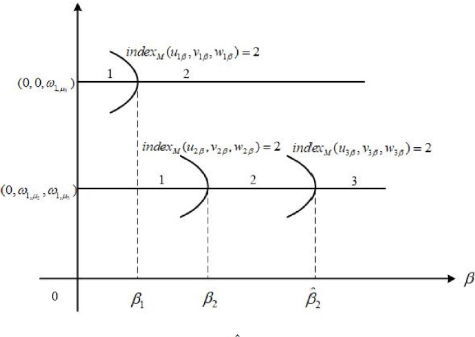
Similar to Theorem (1.2) (ii), we can study the bifurcation solution of (1.1) near (ω1,μ1,0,ω1,μ3) . Using the argument as in Theorem 1.2 (ii), one can obtain the similar results.

Fig. 1

Bifurcation diagram for the system (1.1) when

β1<β2<βˆ2.

From Theorem 1.2, we know that the system (1.1) has the above bifurcation diagram.

Finally, we use the implicit function theorem to study the existence of nontrivial solutions of (1.1). We define

(1.17) A1=(−Δ+λ1−3μ1ωλ1,μ12)−1(ωλ1,μ1ωλ2,μ22+ωλ1,μ1ωλ3,μ3),A2=(−Δ+λ2−3μ2ωλ2,μ22)−1(12ωλ1,μ12ωλ2,μ2+ωλ2,μ2ωλ3,μ3)A3=(−Δ+λ3−3μ3ωλ3,μ3)−112ωλ1,μ12+12ωλ2,μ22,andA4=(−Δ+λ3)−112ωλ1,μ12+12ωλ2,μ22.

Then we have the following results.

Theorem 1.4

Assume that μi>0,λi>0(i=1,2,3) and β₁₂=β₁₃=β₂₃=β. Then there exists τ3>0 such that for β ∈ (− τ ₄, τ ₄), the system (1.1) has seven solutions (u_jβ, v_jβ, w_jβ)(j=4, ..., 10) of the form

(1.18) u4β=ωλ1,μ1+βA1+o(β),v4β=ωλ2,μ2+βA2+o(β),w4β=ω1,μ3+βA3+o(β);u5β=ωλ1,μ1+β−Δ+λ1−3μ1ωλ1,μ12−1ωλ1,μ1ωλ2,μ22+o(β),v5β=ωλ2,μ2+β−Δ+λ2−3μ2ωλ2,μ22−112ωλ1,μ12ωλ2,μ2+o(β),w5β=βA4+o(β);u6β=ωλ1,μ1+β−Δ+λ1−3μ1ωλ1,μ12−1ωλ1,μ1ωλ3,μ3+o(β),v6β=o(β),w6β=ωλ3,μ3+β−Δ+λ3−3μ1ωλ1,μ12−112ωλ1,μ12+o(β);u7β=o(β),v7β=β−Δ+λ2−3μ2ωλ2,μ22−1ωλ2,μ2ωλ3,μ3+o(β),w7β=ωλ3,μ3+β−Δ+λ3−3μ1ωλ1,μ12−112ωλ2,μ22+o(β)

and

(1.19) u8β=o(β),v8β=o(β),w8β=o(β);u9β=o(β),v9β=o(β),w9β=β−Δ+λ3−112ωλ2,μ22+o(β);u10β=o(β),v10β=o(β),w10β=β−Δ+λ3−112ωλ1,μ12+o(β).

When β ∈ (0, τ ₄), all seven solutions above are all positive, and when β ∈ (− τ ₄, 0), the seven solutions have sign patterns (u_4β, v_4β, w_4β)=(+, +, +), (u_5β, v_5β, w_5β)=(+, +, −), (u_6β, v_6β, w_6β)=(+, −, +), (u_7β, v_7β, w_7β)=(−, −, +) and (u_jβ, v_jβ, w_jβ)=(−, −, −)(j=8, 9, 10).

This paper is organized as follows. We give some basic results and prove Theorem 1.1 in Section 2. In Section 3 we discuss the asymptotic behavior of the positive solution of (1.1). Finally, we give the bifurcation results in the last section.

2 Existence of the solutions for the NLS-NLS-KdV system

Throughout the paper, we shall use the following notations.

||.|| is the norm of H¹(ℝ^N) defined by ||u||2=∫RN|∇u|2+u2
||.||_M is an equivalent norm of H¹(ℝ^N) defined by ||u||M2=∫RN|∇u|2+Mu2 for M>0 .
For z=(u, v, w) ∈ X³ := (H¹(ℝ^N))³, we define ||z||X32=||u||λ12+||v||λ22+||w||λ32 , where λi(i=1,2,3)>0 .
|.|_p is the norm of L^p(ℝ^N) defined by |u|p=∫RN|u|p1/p for 0<p≤∞ .
2∗=2NN−2 if N ≥ 3, and 2*=∞ if N=1, 2.
Let c or C denote the different positive constants.

In this section we shall focus on the existence and nonexistence of solution of (1.1). To accomplish this we need some basic conclusions. First, we define

(2.1) Sλ,μ=infu∈X∖{0}||u||λ2μ∫RNu412,Tλ,μ=infu∈M012||u||λ2−μ4∫RNu4

and

(2.2) S˜λ˜,μ˜=infv∈X∖{0}||v||λ˜2μ˜∫RN|v|323 and T˜λ˜,μ˜=infv∈M112||v||λ˜2−μ˜3∫RN|v|3,

where M0={u∈X:u≠0,||u||λ2=μ∫RNu4} and M1={v∈X:v≠0,||v||λ˜2=μ˜∫RN|v|3} . Then the following basic results hold for Sλ,μ,Tλ,μ,S˜λ˜,μ˜ and T˜λ˜,μ˜ .

Lemma 2.1

Assume that λ,λ˜,μ,μ˜>0 ,then T_{𝜆, 𝜇} is attained by the unique positive solution 𝜔_{𝜆, 𝜇}(x) of (1.7) and T˜λ˜,μ˜ is attained by the unique positive solution ωλ˜,μ˜(x) of (1.9). Moreover, we have

(2.3) Tλ,μ=14Sλ,μ2 and Sλ,μ=λ1−N4μ12S1,1=:λ1−N4μ12S1,

(2.4) T˜λ˜,μ˜=16S˜λ˜,μ˜3 and S˜λ˜,μ˜=λ˜1−N6μ˜23S˜1,1=:λ˜1−N6μ˜23S2,

where S1,1=S1=∫RNω0412 , S˜1,1=S2=∫RNω1313 , and 𝜔₀, 𝜔₁ are given in (1.8)-(1.10).

The proof of this lemma can be accomplished by a direct computation. For more details one can refer to [45, Proposition 2.1]. In order to find nontrivial critical points for 𝜙, we define the following Nehari type manifold.

(2.5) N=z=(u,v,w)∈X3∖{(0,0,0)}:Φ′(u,v,w)(u,v,w)=0=z=(u,v,w)∈X3∖{(0,0,0)}:∥u∥λ12+∥v∥λ22+∥w∥λ32=∫RNμ1u4+μ2v4+μ3w3+2∫RNβ12u2v2+32∫RNβ13u2w+β23v2w.

It is easy to see that all nontrivial solutions of (1.1) are constrained in N . We infer from the definition of N that for (u,v,w)∈N and β12>0,μi,λi,i=1,2,3 ,

(2.6) Φ(u,v,w)=16||z||X32+112∫RN(μ1u4+μ2v4)+β126∫RNu2v2≥16||z||X32.

Moreover, for each (u,v,w)∈N , it follows from Hölder and Young’s inequalities that

(2.7) ∥u∥λ12+∥v∥λ22+∥w∥λ32=∫RNμ1u4+μ2v4+μ3w3+2∫RNβ12u2v2+32∫RNβ13u2w+β23v2w≤c∥u∥λ14+∥v∥λ24+∥w∥λ33+∥u∥λ12∥v∥λ22+∥u∥λ12∥w∥λ3+∥v∥λ22∥w∥λ3≤c∥u∥λ14+∥v∥λ24+∥w∥λ33.

for some c > 0. Thus, we deduce from (2.6) and (2.7) that 𝜙 is bounded uniformly away from zero on N .

Before going further we define the ground state energy and radial ground state energy by

(2.8) C=infz∈NΦ(z), Cr=infz∈N∩Xr3Φ(z).

The following lemma shows the role of C and C_r.

Lemma 2.2

Assume that λi,μi>0,β12>0 , β13,β23∈R , if C or C_r is attained by some z0∈N . Then z₀ is a solution of (1.1).

Proof

We take z0=(u0,v0,w0)∈N such that 𝜙(z₀)=C. By [11, Theorem 4.1.1], there exists a Lagrangian multiplier κ∈R such that 𝜙'(z₀)=𝜅 𝜃'(z₀), where 𝜃(z₀)=𝜙'(z₀)z₀. Since z0=(u0,v0,w0)∈N , one deduces that

(2.9) θ′z0z0=2z0X32−4∫RNμ1u4+μ2v4−3∫RNμ3w3−8∫RNβ12u2v2−92∫RNβ13u2w+β23v2w=−z0X32−∫RNμ1u4+μ2v4−2∫RNβ12u2v2<0.

Obviously, 𝜙'(z₀)z₀=0, z0∈N . So, we infer from (2.9) that 𝜅=0. Thus, we have 𝜙'(z₀)=0. In other words, z₀ is a critical point of 𝜙 and is solution of (1.1). □

Next we shall prove a basic existence result. That is, the least level C or C_r is attained by some (possibly semitrivial) z∈N .

Lemma 2.3

Suppose that λi,μi>0(i=1,2,3) , β12>0 and β13,β23∈R . Then C > 0 or C_r > 0 is attained by some z0∈N , where C or C_r is defined in (2.8).

Proof

From (2.6) and (2.7), we know that there exists ε>0 such that C≥ε>0 . Since (0,0,ωλ3,μ3)∈N , it follows that N⋂X3≠∅ . Let {(un,vn,wn)}⊂N be a minimizing sequence. By using the Ekeland’s variational principle-type arguments (see [48] or [47]), there exists a sequence (still denote by {(u_n, v_n, w_n)} on N such that

(2.10) Φ(un,vn)→C and Φ′(un,vn)→0, as n→∞,

which also implies the boundedness of {(u_n, v_n, w_n)} in X³. We can assume that (u_n, v_n, w_n)⇀(u₀, v₀, w₀) in X³ and (u_n, v_n, w_n)→(u₀, v₀, w₀) in [Llocp(RN)]3 for p ∈ (2, 2*).

The sequence {(u_n, v_n, w_n)} is nonvanishing. That is, there exists y_n ∈ ℝ^N and R > 0 such that

(2.11) lim infn→∞∫BR(yn)(un2+vn2+wn2)≥σ>0,

where B_R(y_n)={y ∈ ℝ^N: |y − y_n| ≤ R}. On the contrary, if (2.11) is not satisfied, we have {(u_n, v_n, w_n)} is vanishing, i.e., for any R > 0,

(2.12) limn→∞supy∈RN∫BR(y)(un2+vn2+wn2)=0.

By using the concentration compactness lemma(see [48, Lemma 1.21]), we have u_n→0, v_n→0 and w_n→0 in L^p(ℝ^N) for ∀ p ∈ (2, 2*). Therefore, we infer from 𝜙'(u_n, v_n, w_n)(u_n, v_n, w_n)→0 that

unλ12+vnλ22+wnλ32=∫RNμ1un4+μ2vn4+μ3wn3+2∫RNβ12un2vn2+32∫RNβ13un2wn+β23vn2wn→0,

as n→∞. This implies that

(2.13) 0<ε≤C=16unλ12+vnλ22+wnλ32+112∫RNμ1un4+μ2vn4+β126∫RNun2vn2+o(1)→0.

This is a contradiction. Hence we know that (2.12) holds.

Finally, we prove there exists (u, v, w) ∈ X³\ {(0, 0, 0)} such that 𝜙(u, v, w)=C and 𝜙'(u, v, w)=0. Set u¯n=un(x+yn),v¯n=vn(x+yn) and wˉn=wn(x+yn) . Due to the invariance by translations, we infer that there exists (u_n, v_n, w_n) ∈ X³ such that (uˉn,vˉn,wˉn)⇀(u,v,w) in X³, (uˉn,vˉn,wˉn)→(u,v,w) in [Llocp(RN)]3(∀p∈ (2, 2*)), where u, v, w ≥ 0. Moreover, (2.11) gives that

(2.14) lim infn→∞∫BR(0)(uˉn2+vˉn2+wˉn2)≥σ>0.

Consequently, we know that at least one of uˉ,vˉ and wˉ is nonzero. It is easy to see that 𝜙'(u, v, w)=0 and (u,v,w)∈N∩X3 . Furthermore, by the weak lower semicontinuity of the norms, we know that

C≤Φ(u,v,w)=16∥u∥λ12+∥v∥λ22+∥w∥λ32+112∫RNμ1u4+μ2v4+β126∫RNu2v2≤lim infn→∞16uˉnλ12+vˉnλ22+wˉnλ32+112∫RNμ1uˉn4+μ2vˉn4+β126∫RNuˉn2vˉn2=lim infn→∞Φuˉn,vˉn,wˉn=limn→∞Φun,vn,wn=C.

Hence, z=(u, v, w)≠(0, 0, 0) is a ground state solution of (1.1). Similarly, we prove Cr>0 is attained by some z∈N . This ends the proof. □

From Lemma 2.3, we know that C > 0 is attained by some (u, v, w) ∈ X³\{(0, 0, 0)}. To prove the existence of positive ground state solution of (1.1), it suffices to exclude the semitrivial solutions z=(0, 0, w), (0, v, w) and (u, 0, w). That is, we only need to show that

C=Φ(u,v,w)<minΦ(0,0,w),Φ(0,v,w),Φ(u,0,w).

To accomplish this we first give the following result.

Lemma 2.4

Assume that λi,μi>0,i=1,2,3 and β12>0,β13,β23∈R . For any z=(u, v, w) ∈ X³, there exists a unique number s˜>0 such that Φ(s˜z)=maxs≥0Φ(sz) .

Proof

Let z=(u, v, w) ∈ X³. For any s>0 , we set

F(s)=Φ(sz)=A2s2−B4s4−C6s3,

where

A=∥z∥X32>0,B=∫RNμ1u4+μ2v4+2β12u2v2>0,C=∫RN2μ3w3+3β12u2w+3β23v2w∈R.

Now we prove that F:R+⟼R admits a unique maximum. Let us observe that

lims⟶0+F(s)s2=A2>0, lims⟶∞F(s)=−∞.

Then there exists at least a s˜ such that

F(s˜)=maxs≥0F(s).

Any maximum point of F satisfies

F′(s)=As−Bs3−C2s2=0,

that is,

(2.15) A=Bs2+C2s.

We claim that s˜ is the unique solution of (2.15). In fact, if C ≥ 0, it is easy to see that (2.15) has a unique solution s˜>0 . Suppose C < 0, and we let D=−C,

G(s)=F′(s)s=A−Bs2+D2s,

where s>0 . Let s0=min{s>0|G(s)=0} , we suppose that there exists s1>s0 such that

(2.16) G(s1)=G(s0)=0.

Since lims→0G(s)=A>0 , we have that G′(s0)=−2Bs0+D2≤0 and

(2.17) D2≤2Bs0.

It follows from (2.16) that there exists s₂ ∈ (s₀, s₁) such that G'(s₂)=0. Therefore, from (2.17), we have

D2=2Bs2>2Bs0≥D2,

which yields a contradiction. □

Lemma. 2.5

Assume that λi,μi>0,i=1,2,3 and β₁₂ > 0, there exists β˜>0 such that for any β13+β23>β˜ , (1.1) has a positive ground state solution z=(u, v, w) ∈ X³(or z∈Xr3) .

Proof

We first prove the existence of ground state solution of (1.1) Let w˜∈X be the positive solution of (1.9), u, v ∈ X and u ≠ 0, v ≠ 0. We let (0,0,w˜) , (u,0,w˜) , (0,v,w˜) are semitrivial solutions of (1.1) It follows from (1.6) that

(2.18) Φ(0,0,w˜), Φ(u,0,w˜), Φ(0,v,w˜)>0.

We claim that there exists z ∈ 𝒩 such that

(2.19) Φ(z)<minΦ(0,0,w˜),Φ(0,v,w˜),Φ(u,0,w˜).

Indeed, by Lemma 2.4, we see that there exists sβ:=sβ13,β23>0 such that sβ(u,v,w˜)∈N , then

||z∗||X32=sβ2∫RN(μ1u4+μ2v4+2β12u2v2)+sβ∫RNμ3w˜3+32sβ∫RN(β13u2w˜+β23v2w˜).

where z∗=(u,v,w˜) . Since the last integral is strictly positive, it follows that

(2.20) limβ13+β23→∞sβ=0.

We know that

Φ(sβ(u,v,w˜))=sβ26||z∗||X32+sβ412∫RN(μ1u4+μ2v4+2β12u2v2).

Hence, (2.19) is satiesfied if β₁₃+β₂₃ sufficiently large by (2.18) and (2.20).

Next we prove that there exists a positive ground state solution. Fix β₁₃ + β₂₃ > 0 large enough. Let zˆ=(uˆ,vˆ,wˆ) be a ground state solution of (1.1) and we let z˜=(|uˆ|,|vˆ|,|wˆ|) . From Lemma 2.4, we know that there exists unique sz˜ such that sz˜z˜∈N . Since zˆ,sz˜z˜∈N , if

A=||zˆ||X32 0, B=∫RN(μ1uˆ4+μ2vˆ4+2β12uˆ2vˆ2) 0,C=∫RN(2μ3wˆ3+3β12uˆ2wˆ+3β23vˆ2wˆ)∈R,C˜=∫RN(2μ3|wˆ|3+3β12uˆ2|wˆ|+3β23vˆ2|wˆ|) 0,

we have that

A=B+C2

and

A=Bsz˜2+C˜2sz˜.

Then sz˜≤1 . Since zˆ is a ground state solution of (1.1) and sz˜z˜∈N , we obtain

Φ(zˆ)≤Φ(sz˜z˜)=sz˜26A+sz˜412B≤16A+112B=Φ(zˆ).

Therefore, sz˜z˜ is a ground state solution with non-negative components. By strong maximum principle, repeating the arguments of [45], we infer that each component is positive.

Similarly, we can prove (u,v,w)∈Xr3 is a positive ground state solution under the assumption.

Now we are ready to give the proof Theorem 1.1.

Proof of the Theorem 1.1

From Lemma 2.5, Theorem 1.1 (i) holds. Next we prove the nonexistence of positive solutions. Suppose that (u, v, w) is a positive solution of (1.1) Then we infer from the Pohozaev identity(see [39, Theorem 1]) that for any a∈R ,

(2.21) N2−(a+1)∫RN|∇u|2+|∇v|2+|∇w|2+N2−a∫RNλ1u2+λ2v2+λ3w2+a−N4∫RNμ1u4+μ2v4+2β12u2v2+a−N3∫RNμ3|w|3+3a−N2∫RNβ13u2|w|+β23v2|w|=0

Let a=N2−1 , through substitution by (2.21), then

(2.22) ∫RNλ1u2+λ2v2+λ3w2=4−N4∫RNμ1u4+μ2v4+2β12u2v2+6−N6∫RNμ3|w|3+6−N4∫RNβ13u2|w|+β23v2|w|.

If N=4, λi>0(i=1,2,3),μ3,β13,β23<0 and μ1,μ2,β12∈R , then (2.22) holds if and only if u=v=w=0. If N=5, we know that ∫RNu4=+∞ . then (2.22) holds if and only if u=v=w=0 under the conditions λi>0(i=1,2,3),μ1,μ2,β12≥0 , μ₃, β₁₃, β₂₃ ≤ 0. If N ≥ 6, then ∫RNu4=+∞ and ∫RN|w|3=+∞ , then (2.22) holds if and only if u=v=w=0 under the conditions λi>0(i=1,2,3),μ1,μ2,β12,μ3,β13,β23≥0 . □

3 Bifurcation results for the NLS-NLS-KdV system

In this section we study the bifurcation results of (1.1) For the simplicity we assume that β₁₂=β₁₃=β₂₃=β and λ₁=λ₂=λ₃=1. First, we consider the eigenvalue problem

(3.1) −Δϕ2+ϕ2−(3μ2ω1,μ22+βω1,μ3)ϕ2−βω1,μ2ϕ3=χ(β)ϕ2,−Δϕ3+ϕ3−βω1,μ2ϕ2−2μ3ω1,μ3ϕ3=χ(β)ϕ3.

We define

(3.2) χ(β)=inf∥ϕ2∥2+∥ϕ3∥2−∫RN[(3μ2ω1,μ22+βω1,μ3)ϕ22−2μ3ω1,μ3ϕ32]−2∫RNβω1,μ2ϕ2ϕ3∫RN(ϕ22+ϕ32),

where β > 0 and φ₂, φ₃ ∈ X_r\{0}. The next lemma prove the existence of principal eigenvalue of (3.1).

Lemma. 3.1

Assume that μ₂, μ₃ > 0 and β > 0. Then χ(β) is a unique principal eigenvalue of (3.1), and ϕ⃗β=(ϕ2,β,ϕ3,β) is the correspond positive eigenfunction and χ′(β)<0 . Moreover, if min1−3μ2||ω1,μ22||∞,1−2μ3||ω1,μ3||∞>0 , we get

(3.3) limβ→0+χ(β)>0andlimβ→∞χ(β)=−∞ for β>0.

In particular there exists βˆ2>0 such that χ(βˆ2)=0 , therefore βˆ2 is the principal eigenvalue of (1.13).

Proof

We follow the idea of [47, Lemma 4.1] to prove this conclusion. As in [9, Section 3, Theorem 3.4], we know that the definition of (3.2) is the principal eigenvalue of (3.1). Let φ_β denote the correspond positive eigenfunction. Obviously, (χ(β),ϕ⃗β) is differentiable with respect to β. Differentiating (3.1) in β, one deduces that

(3.4) −Δϕ′2,β+ϕ′2,β−(3μ2ω1,μ22+βω1,μ3)ϕ′2,β−ω1,μ3ϕ2,β−ω1,μ2ϕ3,β−βω1,μ2ϕ′3,β=χ′(β)ϕ2,β+χ(β)ϕ′2,β,−Δϕ′3,β+ϕ′3,β−2μ3ω1,μ3ϕ′3,β−ω1,μ2ϕ2,β−βω1,μ2ϕ′2,β=χ′(β)ϕ3,β+χ(β)ϕ′3,β,

where ϕj,β′=∂ϕj,β∂β(j=2,3) . Multiplying (3.1) by (φ′_2,β, φ′_3,β), multiplying (3.4) by (φ_2,β, φ_3,β), subtracting and integrating, we obtain that

(3.5) ∫RN(ω1,μ3ϕ2,β2+ω1,μ3ϕ2,βϕ3,β)=−χ′(β)∫RNϕ2,β2and∫RNω1,μ3ϕ2,βϕ3,β=−χ′(β)∫RNϕ2,β2.

This implies that χ′(β)<0 . Since ω1,μ2 and ω1,μ3 are bounded for x ∈ ℝ^N, we infer from (3.2) that

∫RN[|∇ϕ2|2+ϕ22+|∇ϕ3|2+ϕ32−(3μ2ω1,μ22+βω1,μ3)ϕ22−2μ3ω1,μ3ϕ32]−2∫RNβω1,μ2ϕ2ϕ3≥∫RNϕ22+ϕ32−3μ2ω1,μ22+βω1,μ3ϕ22−2μ3ω1,μ3ϕ32−2∫RNβω1,μ2ϕ2ϕ3≥∫RN1−3μ2ω1,μ22−βω1,μ3ϕ22+1−2μ3ω1,μ3ϕ32−2∫RNβω1,μ2ϕ2ϕ3≥min1−3μ2||ω1,μ22||∞−β||ω1,μ3||∞,1−2μ3||ω1,μ3||∞∫RN(ϕ22+ϕ32)−β||ω1,μ2||∞∫RN(ϕ22+ϕ32).

Thus, we obtain that limβ→0+χ(β)≥min1−3μ2||ω1,μ22||∞,1−2μ3||ω1,μ3||∞>0 .

For each R > 0, consider the following eigenvalue problem

(3.6) −ΔϕR(y)=λRϕR(y), inBR(0),ϕR(0)=0, on∂BR(0),

where (λ_R, φ_R) be the principal eigen-pair of (3.6), and (3.6) satisfying ∫BR(0)ϕR2=1 . Then we know that λ_R=λ₁R^-2. We extend φ_R to be zero outside of B_R(0), and regard (φ_R, φ_R) as a test function for (3.2). Then we have that for all β > 0 and R > 0, there holds

(3.7) χ(β)≤1+λ1R−2−12∫BR(0)(3μ2ω1,μ22+2μ3ω1,μ3+βω1,μ3+2βω1,μ2)ϕR2.

Since μi,ω1,μi>0(i=2,3) , assume R > 0 is a fixed constant for (3.7), then we have that limβ→∞χ(β)=−∞ . The existence of a unique βˆ2 such that χ(βˆ2)=0 follows immediately from (3.3). □

Now we are ready to give the proof of Theorem 1.2.

Proof of Theorem 1.2

In order to prove the results, we shall use the bifurcation results of Crandall and Rabinowitz [15]. We fist define H: R×Xr3→Yr3 by

(3.8) H(β,u,v,w)=Δu−u+μ1u3+βuv2+βuwΔv− v+μ2v3+βu2v+βvwΔw−w+μ3w2+12βu2+12βv2.

Obviously, for (ϕ1,ϕ2,ϕ3),(ψ1,ψ2,ψ3),(φ1,φ2,φ3)∈Xr3 , a direct computation shows that

(3.9) H(u,v,w)(β,u,v,w)ϕ1,ϕ2,ϕ3=Δϕ1−ϕ1+3μ1u2ϕ1+βϕ1v2+2βuvϕ2+βϕ1w+βuϕ3Δϕ2−ϕ2+3μ2v2ϕ2+2βuvϕ1+βu2ϕ2+βϕ2w+βvϕ3Δϕ3−ϕ3+2μ3wϕ3+βuϕ1+βvϕ2,H(u,v,w)(u,v,w)(β,u,v,w)[(ϕ1,ϕ2,ϕ3),(ψ1,ψ2,ψ3)]=6μ1uϕ1ψ1+2βϕ1ψ2v+2βψ1ϕ2v+2βψ2ϕ2u+βϕ1ψ3+βϕ3ψ16μ2vϕ2ψ2+2βϕ1ψ1v+2βϕ1ψ2u+2βψ1ϕ2u+βϕ2ψ3+βϕ3ψ22μ3ϕ3ψ3+βϕ1ψ1+βϕ2ψ2,H(u,v,w)(u,v,w)(u,v,w)(β,u,v,w)[(ϕ1,ϕ2,ϕ3),(ψ1,ψ2,ψ3),(φ1,φ2,φ3)]=6μ1ϕ1ψ1φ1+2βϕ1ψ2φ2+2βψ1ϕ2φ2+2βψ2ϕ2φ16μ2ϕ2ψ2φ2+2βϕ1ψ1φ2+2βϕ1ψ2φ1+2βψ1ϕ2φ10,Hβ(β,u,v,w)=uv2+uwu2v+vw12u2+12v2,

and

(3.10) Hβ(u,v,w)(β,u,v,w)[(ϕ1,ϕ2,ϕ3)]=v2ϕ1+2uvϕ2+wϕ1+uϕ32uvϕ1+u2ϕ2+wϕ2+vϕ3uϕ1+vϕ2.

To accomplish the results we divide into the following three cases.

Case 1 We first consider the bifurcation of nontrivial solution of (1.1) from the semi-trivial branch S near (β1,0,0,ω1,μ3) , where S={(β,u,v,w):β>0} and β₁ > 0 is given in (1.11). To this purpose we define

L1[(ϕ1,ϕ2,ϕ3)]=H(u,v,w)(β1,0,0,ω1,μ3)[(ϕ1,ϕ2,ϕ3)]=Δϕ1−ϕ1+β1ω1,μ3ϕ1Δϕ2−ϕ2+β1ω1,μ3ϕ2Δϕ3−ϕ3+2μ3ω1,μ3ϕ3.

From [30, Lemma 2.1], we know that the only solution of Δϕ3−ϕ3+2μ3ω1,μ3ϕ3=0 in X_r is 0. Then N(L1)=span{(ϕβ1,ϕβ1,0)} , and ϕβ1 is the principal eigenfunction of (1.11). Correspondingly, the rang space of L1 is defined by

R(L1)=(f1,f2,f3)∈Yr3:∫RN(f1+f2)ϕβ1=0.

Then dim N(L1)=codimR(L1)=1 . Since ∫RNω1,μ3ϕβ1>0 , we deduce from (3.10) that

Hβ(u,v,w)(β1,0,0,ω1,μ3)[(ϕβ1,ϕβ1,0)]=ω1,μ3ϕβ1ω1,μ3ϕβ10∉R(L1).

By applying the result of [15], we have that the set of positive solution to (1.1) near (β1,0,0,ω1,μ3) is smooth curve

Γ1=(β(s),u1β(s),v1β(s),w1β(s)):s∈(0,τ1),

such that β(s)=β+β′(0)s+12β′′(0)s2+o(s2),uβ(s)=sϕβ1+o(s2) , v1β(s)=sϕβ1+o(s2) and w1β(s)=ω1,μ3+o(s2) , where τ1>0 is a small constant. β′(0) can be calculated as (see [22,44])

(3.11) β′(0)=−〈H(u,v,w)(u,v,w)(β1,0,0,ω1,μ3)[(ϕβ1,ϕβ1,0),(ϕβ1,ϕβ1,0)],ℓ1〉2〈Hβ(u,v,w)(β1,0,0,ω1,μ3)[(ϕβ1,ϕβ1,0)],ℓ1〉=0,

and

(3.12) β′′(0)=−〈H(u,v,w)(u,v,w)(u,v,w)(β1,0,0,ω1,μ3)[(ϕβ1,ϕβ1,0),(ϕβ1,ϕβ1,0),(ϕβ1,ϕβ1,0)],ℓ1〉3〈Hβ(u,v,w)(β1,0,0,ω1,μ3)[(ϕβ1,ϕβ1,0)],ℓ1〉=−∫RN(μ1+μ2+2β1)ϕβ14∫RNω1,μ3ϕβ12<0,

where ℓ₁ is a linear functional on Y³ defined as 〈(f1,f2,f3),ℓ1〉=∫RN(f1+f2)ϕβ1 . Hence we infer from (3.11)-(3.12) that (1.1) has positive solution (u_1β, v_1β, w_1β), where (u_1β, v_1β, w_1β) in the form of (1.14) for β1−τ1<β<β1 . Furthermore, from the special structure form of the system (1.1), we know that the (u_1β, -v_1β, w_1β) and (-u_1β, ± v_1β, w_1β) are also a solution of (1.1)

Next we use [16, Corollary 1.13 and Theorem 1.16] to calculate the Morse index for the nonnegative solution (0,0,ω1,μ3) . For the eigenvalue problem

(3.13) Lβϕ1ϕ2ϕ3=H(u,v,w)(β,0,0,ω1,μ3)[(ϕ1,ϕ2,ϕ3)]=Δϕ1−ϕ1+βω1,μ3ϕ1Δϕ2−ϕ2+βω1,μ3ϕ2Δϕ3−ϕ3+2μ3ω1,μ3ϕ3=L˜1(ϕ1)L˜2(ϕ2)L˜3(ϕ3)=M(β)ϕ1ϕ2ϕ3,

where M(β):(β1−τ0,β1+τ0)→R is simple eigenvalue of Lβ satisfying M(β₁)=0. Notice that the eigenvalues of the problem (3.13) is given by σp(Lβ)=σp(L˜1)⋃σp(L˜2)⋃σp(L˜3) , where σp(L˜i) denotes the eigenvalues of a linear operator L˜i,i=1,2,3 . We need to prove that M′(β)>0 . To the following eigenvalue problem

(3.14) −Δϕ+ϕ−βω1,μ3ϕ=θ(β)ϕ, ϕ∈Xr:=Hr(RN).

Similarly, there exists the principle eigenvalue θ(β) of (3.14) by ([16, Teorem 1.16]), and φ_β denotes the correspond principle eigenfunction. It is easy to see that (θ(β), φ_β) is differentiable with respect to β. Visibly, we have that θ′(β)<0 . And M(β) is determined by L˜ or L˜2 and L˜3 , hence M(β)=-θ(β) defined in (3.13). Thus M′(β)>0 from (3.14).

Now consider the eigenvalue problem at the bifurcating solution (u_1β, v_1β, w_1β):

(3.15) H(u1β,v1β,w1β)(β,u1β,v1β,w1β)[(ϕ1,ϕ2,ϕ3)]=Δϕ1−ϕ1+3μ1u1β2ϕ1+βϕ1v1β2+2βu1βv1βϕ2+βϕ1w1β+βu1βϕ3Δϕ2−ϕ2+3μ2v1β2ϕ2+2βu1βv1βϕ1+βu1β2ϕ2+βϕ2w1β+βv1βϕ3Δϕ3−ϕ3+2μ3w1βϕ3+βu1βϕ1+βv1βϕ2=μ(s)ϕ1ϕ2ϕ3.

Then from [16, Theorem 1.16], we have

lims→0,μ(s)≠0=−sβ′(s)M′(β1)μ(s)=1.

From (3.11)-(3.12) we know that β(0)=β1>0,β′(0)=0 and β′′(0)<0 . So, 0 is the local maximum point of β. β′(s)<0 for s ∈ (-τ₀, 0) and β′(s)>0 for s ∈ (0, τ₀). Consequently, we get that μ(s)>0 for s ∈ (-τ₀, 0)∪(0, τ₀), where τ0>0 sufficiently small.

According to [8], L˜3 has exactly one positive eigenvalue for β > 0 (note that L3 is independent of β). Therefore Lβ has exactly one positive eigenvalues when β ∈ (0, β₁), and has exactly two positive eigenvalues when β ∈ (β₁, β₁+τ₀) for small τ0>0 . From μ(s)>0 and the continuity of eigenvalues, we know that the eigenvalue problem (3.15) has two eigenvalue when s ∈ (-τ₀, 0)∪(0, τ₀). From the definition of Morse index, we know that index_M(u_1β, v_1β, v_1β)=2 for β ∈ (β₁-τ₀, β₁).

Case 2 We give the the result at the bifurcation point (β,0,ω1,μ2,ω1,μ3) . Define

Lβ[(ϕ1,ϕ2,ϕ3)]=H(u,v,w)(β,0,ω1,μ2,ω1,μ3)[(ϕ1,ϕ2,ϕ3)]=Δϕ1−ϕ1+β(ω1,μ22+ω1,μ3)ϕ1Δϕ2−ϕ2+(3μ2ω1,μ22+βω1,μ3)ϕ2+βω1,μ2ϕ3Δϕ3−ϕ3+2μ3ω1,μ3ϕ3+βω1,μ2ϕ2,L∗[(ϕ2,ϕ3)]=Δϕ2−ϕ2+(3μ2ω1,μ22+βω1,μ3)ϕ2+βω1,μ2ϕ3Δϕ3−ϕ3+2μ3ω1,μ3ϕ3+βω1,μ2ϕ2.

According to Lemma 3.1, let βˆ2>0 be the principal eigenvalue of (1.13) and the principle eigenfunction ϕβ2 is radial positive function. The null space of Δϕ1−ϕ1+β2(ω1,μ22+ω1,μ3)ϕ1=0 is span{ϕβ2} (see [30,47]). Since β2≠βˆ2 , then there are two possible bifurcation points (β2,0,ω1,μ2,ω1,μ3) and (βˆ2,0,ω1,μ2,ω1,μ3) . We first consider the result at the bifurcation point (β2,0,ω1,μ2,ω1,μ3) . Obviously, N(Lβ2)=span{ϕβ2,0,0} . And the rang space of Lβ2 is

R(Lβ2)=(f1,f2,f3)∈Yr3:∫RNf1ϕβ2=0.

Therefore dimN(Lβ2)=codimR(Lβ2)=1 . we know from (3.10) that

Hβ(u,v,w)(β2,0,ω1,μ2,ω1,μ3)[(ϕβ2,0,0)]=(ω1,μ22+ω1,μ3)ϕβ200∉R(Lβ2).

Then we have that the set of positive solution to (1.1) near (β2,0,ω1,μ2,ω1,μ3) is smooth curve

(3.16) Γ2=(β(s),u2β(s),v2β(s),w2β(s)):s∈(0,τ2),

such that β(s)=β+β′(0)s+12β′′(0)s2+o(s2),u2β(s)=sϕβ2+o(s2) , v2β(s)=ω1,μ2+o(s2) and w2β(s)=ω1,μ3+o(s2) , where τ2>0 is a small constant. Moreover β′(0) can be calculated as (see [22,44])

(3.17) β′(0)=−〈H(u,v,w)(u,v,w)(β2,0,ω1,μ2,ω1,μ3)[(ϕβ2,0,0),(ϕβ2,0,0)],l2〉2〈Hβ(u,v,w)(β2,0,ω1,μ2,ω1,μ3)[(ϕβ2,0,0)],l2〉=0

and

(3.18) β′′(0)=−〈H(u,v,w)(u,v,w)(u,v,w)(β2,0,ω1,μ2,ω1,μ3)[(ϕβ2,0,0),(ϕβ2,0,0),(ϕβ2,0,0)],l2〉3〈Hβ(u,v,w)(β2,0,ω1,μ2,ω1,μ3)[(ϕβ2,0,0)],l2〉=−2∫RNμ1ϕβ24∫RN(ω1,μ22+ω1,μ3)ϕβ22<0,

where ℓ₂ is a linear functional on Y³ defined as 〈(f1,f2,f3),ℓ2〉=∫RNf1ϕβ2 . Thus from (3.16)-(3.18) we get that (1.1) has a positive solution (u_2β, v_2β, w_2β) in the form of (1.15) for β2−τ2<β<β2 . As in Case 1, we know that (u_2β, −v_2β, w_2β) and (u_2β, ± v_2β, w_2β) are also solutions of (1.1).

Next we consider the result at the bifurcation point (βˆ2,0,ω1,μ2,ω1,μ3) . we have N(Lβˆ2)=span{0,ϕ2,βˆ2,ϕ3,βˆ2} . And the rang space of Lβˆ2 is

R(Lβˆ2)=(f1,f2,f3)∈Yr3:∫RN(f2ϕ2,βˆ2+f3ϕ3,βˆ2)=0.

Therefore dimN(Lβˆ2)=codimR(Lβˆ2)=1 . From (3.10), one deduces that

Hβ(u,v,w)(β2,0,ω1,μ2,ω1,μ3)[0,ϕ2,βˆ2,ϕ3,βˆ2]=0ω1,μ2ϕ2,βˆ2+ω1,μ3ϕ3,βˆ2ω1,μ2ϕ2,βˆ2∉R(Lβˆ2).

Then we have that the set of positive solution to (1.1) near (βˆ2,0,ω1,μ2,ω1,μ3) is smooth curve

(3.19) Γ3=(β(s),u3β(s),v3β(s),w3β(s)):s∈(0,τ3),

such that β(s)=β+β′(0)s+o(s), u_3β(s)=s+o(s), v3β(s)=ω1,μ2+ϕ2,βˆ2s+o(s) and w3β(s)=ω1,μ3+ϕ3,βˆ2s+o(s) , where τ3>0 is a small constant. As in the above, we know that β′(0) has the form

(3.20) β′(0)=−〈H(u,v,w)(u,v,w)(βˆ2,0,ω1,μ2,ω1,μ3)[(0,ϕ2,βˆ2,ϕ3,βˆ2),(0,ϕ2,βˆ2,ϕ3,βˆ2)],ℓ3〉2〈Hβ(u,v,w)(βˆ2,0,ω1,μ2,ω1,μ3)[(0,ϕ2,βˆ2,ϕ3,βˆ2)],ℓ3〉=−∫RN(6μ2ω1,μ2ϕ2,βˆ23+2μ3ϕ2,βˆ22ϕ3,βˆ2+3βˆ2ϕ3,βˆ23)2∫RN(2ω1,μ2ϕ2,βˆ2ϕ3,βˆ2+ω1,μ3ϕ2,βˆ22)<0,

where ℓ₃ is a linear functional on Y³ defined as 〈(f1,f2,f3),ℓ3〉=∫RN(f2ϕ2,βˆ2+f3ϕ3,βˆ2) . Thus from (3.19)-(3.20), we get that (1.1) has a positive solution (w_3β, v_3β, w_3β) in the form of (1.16) for ϕβˆ2−τ3<β<ϕβˆ2 . Similar to the case 1, the Morse index can be calculated. Here we omit the details. □

Finally, we give the proof of Theorem 1.4.

Proof of Theorem 1.4

For the convenience of notations, we set u1(x)=ωλ1,μ1(x),v1(x)=ωλ2,μ2(x) and w1(x)=ωλ3,μ3(x) , where ωλj,μj(j=1,2,3) is defined in (1.8)-(1.10). Obviously, we know that if β=0, then the system (1.1) has the following seven nonnegative solutions

z1=(u1,v1,w1), z2=(u1,v1,0), z3=(u1,0,w1), z4=(0,v1,w1)andz5=(u1,0,0), z6=(0,v1,0), z7=(0,0,w1).

We shall apply the implicit function theorem at z_j with parameter β=0 for j=1, ···, 7. Since the proof is essentially the same for each of j=1, ···, 7, we only present the proof for z₁. Since z₁ is non-degenerate in Xr3,i.e.,[H(u,v,w)(0,z1)]−1 exists, we infer from the implicit function theorem that there exist β˜>0,R1>0 and zˆ1(β):(−β˜,β˜)→BR1(z1) such that for any β∈(−β˜,β˜),H(β,zˆ1(β))=H(β,uˆ1(β),vˆ1(β),wˆ1(β))=0 , where H is defined in (3.8). Moreover we can solve (ϕ₁, ϕ₂, ϕ₃) from is the unique positive solution of (1.1) with β=0. One infers from (3.9) that

H(u,v,w)(0,u1,v1,w1)[(ϕ1,ϕ2,ϕ3)]=Δϕ1−ϕ1+3μ1u12ϕ1Δϕ2−ϕ2+3μ2v12ϕ2Δϕ3−ϕ3+2μ3w1ϕ3=−u1v12+u1w1u12v1+v1w112u12+12v12.

Hence one has that

(3.21) ϕ1=(−Δ+λ1−3μ1u12)−1(u1v12+u1w1), ϕ2=(−Δ+λ2−3μ2v12)−1(12u12v1+v1w1),ϕ3=12(−Δ+λ3−2μ3w1)−1(u12+v12).

From (3.21), we can give the expression of (u_4β, v_4β, w_4β) in (3.18). Similarly, by using the implicit function theorem at semitrivial solution z_i(i=2, ···, 7), we can get the positive solutions (u_jβ, v_jβ, w_jβ)(j=5, ···, 10) as in (1.18)-(1.19).Hence, there exists τ4>0 such that when β ∈ (0, τ₄), (1.1) has exactly seven positive solutions. If β ∈ (−τ₄, 0), and the sign information of (u_jβ, v_jβ, w_jβ) with j=4, 5, 6, 7, 8, 9, 10 can be obtained by the form in (1.18)-(1.19).

Acknowledgement

The authors thank Prof. Junping Shi for many useful discussion. J. Wang was supported by NSF of China (Grants 11971202), Outstanding Young Foundation of Jiangsu Province (BK20200042), the Six big talent peaks project in Jiangsu Province(XYDXX-015). Q.-P. Geng was supported by the research and innovation plan for Postgraduates in Jiangsu Province (KYCX20_286). The authors would like to thank the referees for several valuable comments and suggestions which helped to improve this paper.

Data availability: No data were used to support this study.
Competing interests: The authors declare that they have no competing interests.
Authors' contributions: The authors contributed equally in this article. They have all read and approved the final manuscript.

References

[1] N. Akhmediev and A. Ankiewicz, Solitons, Nonlinear pulses and beams, Champman and Hall, London, 1997.Search in Google Scholar

[2] J. Albert and J. Angulo Pava, Existence and stability of ground-state solutions of a Schrödinger-KdV system, Proc. Roy. Soc. Edinburgh Sect. A., 133 (2003), 987-1029.10.1017/S030821050000278XSearch in Google Scholar

[3] A. Ambrosetti, A note on nonlinear Schrödinger systems: existence of a-symmetric solutions, Adv. Nonlinear Stud., 6 (2006), 149-155.10.1515/ans-2006-0202Search in Google Scholar

[4] A. Ambrosetti and E. Colorado, Bound and ground states of coupled nonlinear Schrödinger equations, C. R. Math. Acad. Sci., 342 (2006), 453-458.10.1016/j.crma.2006.01.024Search in Google Scholar

[5] A. Ambrosetti and E. Colorado, Standing waves of some coupled nonlinear Schrödinger equations, J. Lond. Math. Soc., 75 (2007), 67-82.10.1112/jlms/jdl020Search in Google Scholar

[6] H. Amann, Global existence for semilinear parabolic systems, J. Reine Angew. Math., 360 (1985), 47-83.10.1515/crll.1985.360.47Search in Google Scholar

[7] T. Bartsch and Z.-Q. Wang, Note on ground states of nonlinear Schrödinger systems, J. Partial Differential Equations, 19 (2006), 200-207.Search in Google Scholar

[8] P.-W. Bates and J.-P. Shi, Existence and instability of spike layer solutions to singular perturbation problems, J. Funct. Anal., 196 (2002), 211-264.10.1016/S0022-1236(02)00013-7Search in Google Scholar

[9] F.-A. Berezin and M.-A. Shubin, The Schrödinger equation, volume 66 of Mathematics and its Applications (Soviet Series), Kluwer Academic Publishers Group, Dordrecht, 1991.Search in Google Scholar

[10] S. Bhattarai, A. J. Corcho and M. Panthee, Well-Posedness for Multicomponent Schrödinger- gKdV Systems and Stability of Solitary Waves with Prescribed Mass, J. Dyn. Diff. Equat., 30 (2018), 845-881.10.1007/s10884-018-9660-4Search in Google Scholar

[11] K.-C. Chang, Methods in Nonlinear Analysis, Springer Monographs in Mathematics, Springer, Berlin (2005).Search in Google Scholar

[12] S.-M. Chang, C.-S. Lin, T.-C. Lin and W.-W. Lin, Segregated nodal domains of two-dimensional multispecies Bose-Einstein condensates, Physica D: Nonlinear Phenomena, 196 (2004), 341-361.10.1016/j.physd.2004.06.002Search in Google Scholar

[13] Z. Chen, Solutions of nonlinear Schrödinger systems, Dissertation, Tsinghua University, Beijing, Springer Theses. Springer, Heidelberg, 2015.10.1007/978-3-662-45478-7Search in Google Scholar

[14] Z.-J. Chen and W.- M. Zou, An optimal constant for the existence of least energy solutions of a coupled Schrödinger system, Calc. Var. Partial Differential Equations, 48 (2013), 695711.10.1007/s00526-012-0568-2Search in Google Scholar

[15] M.-G. Crandall and P.-H. Rabinowitz, Bifurcation from simple eigenvalues, J. Functional Analysis, 8 (1971), 321-340.10.1016/0022-1236(71)90015-2Search in Google Scholar

[16] M.-G. Crandall and P.-H. Rabinowitz, Bifurcation, perturbation of simple eigenvalues and linearized stability, Arch. Rational Mech. Anal., 52 (1973), 161-180.10.1007/BF00282325Search in Google Scholar

[17] E. Colorado, Existence of bound and ground states for a system of coupled nonlinear Schrödinger-KdV Equations, C. R. Acad. Sci. Paris Ser. I Math., 353 (2014), 511-516.10.1016/j.crma.2015.03.011Search in Google Scholar

[18] E. Colorado, On the existence of bound and ground states for some coupled nonlinear Schrödinger-Korteweg-de Vries equations, Adv. Nonlinear Anal., 6 (2017), 407-426.10.1515/anona-2015-0181Search in Google Scholar

[19] A.-J. Corcho and F. Linares, Well-posedness for the Schrödinger-Korteweg-de Vries system, Trans. Amer. Math. Soc., 359 (2007), 4089-4106.10.1090/S0002-9947-07-04239-0Search in Google Scholar

[20] N. Dancer, K. Wang and Z. Zhang, Uniform Höder estimate for singularly perturbed parabolic systems of Bose-Einstein condensates and competing species, J. Differ. Equ., 251 (2011), 2737-2769.10.1016/j.jde.2011.06.015Search in Google Scholar

[21] J.-P. Dias, M. Figueira and F. Oliveira, Existence of bound states for the coupled Schrödinger-KdV system with cubic nonlinearity, C. R. Math. Acad. Sci. Paris., 348 (2010), 1079-1082.10.1016/j.crma.2010.09.018Search in Google Scholar

[22] Y.-H. Du and J.-P. Shi, Allee efiect and bistability in a spatially heterogeneous predatorprey model, Trans. Amer. Math. Soc., 359 (2007), 4557-4593.10.1090/S0002-9947-07-04262-6Search in Google Scholar

[23] X.-D. Fang, J.-J. Zhang, Multiplicity of positive solutions for quasilinear elliptic equations involving critical nonlinearity, Adv. Nonlinear Anal., 9 (2020), 1420-1436.10.1515/anona-2020-0058Search in Google Scholar

[24] J. Földes and P. Polacik, On cooperative parabolic systems: Harnack inequalities and asymptotic symmetry, Discrete Contin. Dyn. Syst., 25 (2009), 133-157.10.3934/dcds.2009.25.133Search in Google Scholar

[25] M. Funakoshi and M. Oikawa, The resonant Interaction between a Long Internal Gravity Wave and a Surface Gravity Wave Packet, J. Phys. Soc. Japan., 52 (1983), 1982-1995.10.1143/JPSJ.52.1982Search in Google Scholar

[26] Q.-P. Geng, M. Liao, J. Wang and L. Xiao, Existence and bifurcation of nontrivial solutions for the coupled nonlinear Schrödinger-Korteweg-de Vries system, Z. Angew. Math. Phys., 71 (2020), 3310.1007/s00033-020-1256-2Search in Google Scholar

[27] V. Karpman, On the dynamics of sonic-Langmuir solitons, Phys. Scripta., 11 (1975), 263-265.10.1088/0031-8949/11/5/003Search in Google Scholar

[28] T. Kawahara, N. Sugimoto and T. Kakutani, Nonlinear interaction between short and long capillarygravity waves, Stud. Appl. Math., 39 (1975), 1379-1386.10.1143/JPSJ.39.1379Search in Google Scholar

[29] K. Kurata and Y. Osada, Asymptotic expansion of the ground state energy for nonlinear Schrödinger system with three wave interaction, Communications on Pure Applied Analysis, 2021 doi:10.3934/cpaa.2021157.10.3934/cpaa.2021157Search in Google Scholar

[30] L.-S. Lin, Z.-L. Liu and S.-W. Chen, Multi-bump solutions for a semilinear Schrödinger equation, Indiana Univ. Math. J., 58 (2009), 1659-1689.10.1512/iumj.2009.58.3611Search in Google Scholar

[31] T.-C. Lin and J.-C. Wei, Spikes in two coupled nonlinear Schrödinger equations, Ann. I. H. Poincaré-AN, 22 (2005), 403-439.10.1016/j.anihpc.2004.03.004Search in Google Scholar

[32] Z.-L. Liu and Z.-Q. Wang, Ground states and bound states of a nonlinear Schrödinger system, Adv. Nonlinear Stud., 10 (2010), 175-193.10.1515/ans-2010-0109Search in Google Scholar

[33] C.-G. Liu and Y.-Q. Zheng, On soliton solutions to a class of Schrödinger-KdV systems, Proceedings of the American Mathematical Society, 141 (2013), 3477-3484.10.1090/S0002-9939-2013-11629-1Search in Google Scholar

[34] F. Merle and H. Zaag, A Liouville theorem for vector-valued nonlinear heat equations and applications, Math. Ann., 316 (2000), 103-137.10.1007/s002080050006Search in Google Scholar

[35] J. Morgan, Global existence for semilinear parabolic systems, SIAM J. Math. Anal., 20 (1989), 1128-1144.10.1137/0520075Search in Google Scholar

[36] Q.-H. Phan, Optimal Liouville-type theorem for a parabolic system, Discrete Contin. Dyn. Syst., 35 (2015), 399-409.10.3934/dcds.2015.35.399Search in Google Scholar

[37] Q.-H. Phan and P. Souplet, A Liouville-type theorem for the 3-dimensional parabolic Gross–Pitaevskii and related systems, Math. Ann., 366 (2016), 1561-1585.10.1007/s00208-016-1368-3Search in Google Scholar

[38] A. Pomponio, Ground states for a system of nonlinear Schrödinger equations with three wave interaction, J. Math. Phys., 51 (2010), 093513.10.1063/1.3486069Search in Google Scholar

[39] P. Pucci and J. Serrin, A general variational identity, Indiana Univ. Math. J., 35 (1986), 681-703.10.1512/iumj.1986.35.35036Search in Google Scholar

[40] P. Quittner, Liouville theorems for scaling invariant superlinear parabolic problems with gradient structure, Math. Ann., 364 (2016), 269-292.10.1007/s00208-015-1219-7Search in Google Scholar

[41] C. Rüegg, N. Cavadini, A. Furrer, H.-U. Güdel, K. Krämer, H. Mutka, A. Wildes, K. Habicht and P. Vorderwisch, Bose-Einstein condensation of the triple states in the magnetic insulator TlCuCl3, Nature, 423 (2003), 62-65.10.1038/nature01617Search in Google Scholar PubMed

[42] Y. Sato and Z.-Q. Wang, Least energy solutions for nonlinear Schrödinger systems with mixed attractive and repulsive couplings, Adv. Nonlinear Stud., 15 (2015), 1-22.10.1515/ans-2015-0101Search in Google Scholar

[43] Y. Sato and Z.-Q. Wang, Multiple positive solutions for Schrödinger systems with mixed couplings, Calc. Var. Partial Differ. Equ., 54 (2015), 1373-1392.10.1007/s00526-015-0828-zSearch in Google Scholar

[44] J.-P. Shi, Persistence and bifurcation of degenerate solutions, J. Funct. Anal., 169 (1999), 494-531.10.1006/jfan.1999.3483Search in Google Scholar

[45] B. Sirakov, Least Energy Solitary Waves for a System of Nonlinear Schrödinger Equations in ℝⁿ Commun. Math. Phys., 271 (2007), 199-221.10.1007/s00220-006-0179-xSearch in Google Scholar

[46] J. Wang, Solitary waves for coupled nonlinear elliptic system with nonhomogeneous nonlinearities, Calc. Var. Partial Differential Equations, 56 (2017), 38.10.1007/s00526-017-1147-3Search in Google Scholar

[47] J. Wang and J.-P. Shi, Standing waves of coupled Schrödinger equations with quadratic interactions from Raman ampliflcation in a plasma, Submitted, 2018.Search in Google Scholar

[48] M. Willem, Minimax theorems, Progress in Nonlinear Differential Equations and their Applications, 24, Birkahäuser Boston Inc. Boston, MA, 1996.Search in Google Scholar

[49] T.-F. Wu, On a class of nonlocal nonlinear Schrödinger equations with potential well, Adv. Nonlinear Anal., 9 (2020), 665-689.10.1515/anona-2020-0020Search in Google Scholar

[50] A.-L. Xia, Multiplicity and concentration results for magnetic relativistic Schrödinger equations, Adv. Nonlinear Anal., 9 (2020), 1161-1186.10.1515/anona-2020-0044Search in Google Scholar

[51] N. Yajima and M. Oikawa, Formation and interaction of sonic-Langmuir solitons: inverse scattering method, Progr. Theoret. Phys., 56 (1976), 1719-1739.10.1143/PTP.56.1719Search in Google Scholar

Received: 2021-09-27

Accepted: 2021-10-13

Published Online: 2021-11-23

This work is licensed under the Creative Commons Attribution 4.0 International License.

Articles in the same Issue

https://doi.org/10.1515/anona-2021-0214

Keywords for this article

Positive solutions; Bifurcation theory; Critical points; Nonlinear Schrödinger-Korteweg-de Vries system

Creative Commons

BY 4.0