Lower and upper estimates of semi-global and global solutions to mixed-type functional differential equations

J. Diblík; G. Vážanová

doi:10.1515/anona-2021-0218

Artikel Open Access

Lower and upper estimates of semi-global and global solutions to mixed-type functional differential equations

J. Diblík und G. Vážanová

Veröffentlicht/Copyright: 14. Februar 2022

Veröffentlicht von

Veröffentlichen auch Sie bei De Gruyter Brill

Manuskript einreichen Informationen für Autor*innen Erkunden Sie dieses Fachgebiet

Aus der Zeitschrift Advances in Nonlinear Analysis Band 11 Heft 1

Abstract

In the paper, nonlinear systems of mixed-type functional differential equations are analyzed and the existence of semi-global and global solutions is proved. In proofs, the monotone iterative technique and Schauder-Tychonov fixed-point theorem are used. In addition to proving the existence of global solutions, estimates of their co-ordinates are derived as well. Linear variants of results are considered and the results are illustrated by selected examples.

Keywords: Mixed-type functional differential equation; delayed argument; advanced argument; semi-global solution; global solution; monotone iterative method; fixed-point theorem

MSC 2010: Primary: 34K07; 34K25; Secondary: 34K60

1 Introduction

In the paper, the existence is considered of semi-global and global solutions to what is called mixed-type (or advanced-delayed) functional differential equations. Although the existence of global solutions to various classes of functional differential equations has been investigated for some time, most of the papers only deal with semi-global solutions of delayed equations or advanced equations, or with mixed-type equations on finite intervals.

Mixed-type functional differential equations are considered, for example, in the books [1, 18, 30] and in the papers [2, 3, 5, 6, 7, 13, 16, 22, 23, 24, 25, 26, 28, 32]. In [25], exponential dichotomies and Wiener-Hopf factorizations for mixed type equations are discussed. The paper [5] develops monotonic iterations to find solutions to systems exhibiting bistable dynamics while [28] applies a fixed-point technique to determine asymptotic properties of linear mixed-type equations on right-infinite intervals.

Such types of mixed-type equations have found applications in various fields such as optimal control problems, biology, traveling wawes, and economics (we refer, for example, to [2, 5, 6, 7, 22, 25, 30, 32] and to the references therein).

1.1 Preliminaries

By ℝ⩾0n(ℝ>0n) we denote the set of all component-wise nonnegative (positive) vectors v in ℝⁿ, i.e., v = (v₁, . . . , v_n) with v_i ≥ 0 (v_i > 0) for i = 1, . . . , n. For u, v ∈ ℝⁿ, we denote u ≤ v if v−u∈ℝ⩾0n and u < v if u ≤ v and u ≠ v. If, in the paper, inequalities v ≥ u or v > u are used, we assume that they are equivalent with u ≤ v or u < v. In order to avoid unnecessary additional definitions, we use, whenever the meaning is not ambiguous, the same symbols ℝ⩾0n(ℝ>0n) to denote the relevant subsets of the set ℝⁿ.

Let 𝒥 ⊆ ℝ be an interval. By C (𝒥, ℝⁿ) denote the Banach space of bounded continuous functions from 𝒥 to ℝⁿ equipped with the norm ∥ψ∥_r = sup_α∈𝒥 |ψ(α)| where ψ ∈ C (𝒥, ℝⁿ) with the last norm (used throughout the paper) being defined by |ψ(α)| := max{|ψ₁(α)|, . . . , |ψ_n(α)|}. If 𝒥 := [0, r], where r > 0 is fixed, the relevant Banach space is denoted by C_r.

For a function y, continuous on an interval [t − r₁, t], t ∈ ℝ, r₁ > 0, define a delayed-type function y_t ∈ C_r₁ by y_t(τ) = y(t − τ) where τ ∈ [0, r₁]. Similarly, for a function y, continuous on an interval [t, t + r₂], t ∈ ℝ, r₂ > 0, define an advanced-type function y^t ∈ C_r₂ by y^t (σ) = y(t + σ) where σ ∈ [0, r₂].

Let t₀ ∈ ℝ be fixed and let 𝒥 ⊆ ℝ be a set having one of the forms 𝒥 = 𝒥⁺ := [t₀, ∞), 𝒥 = 𝒥⁻ := (−∞, t₀] or 𝒥 = ℝ. In the paper, we will consider a system of mixed-type functional differential equations

(1.1) y˙(t)=f(t,yt,yt)

where y = (y₁, . . . , y_n), f = (f₁, . . . , f_n) : 𝒥 × C_r₁ × C_r₂ → ℝⁿ is a continuous quasi-bounded functional which satisfies a local Lipschitz condition with respect to the second and the third arguments in the domains considered. The well-known definitions of quasi-boundedness and local Lipschitz condition can be found, e.g., in [15].

We say that a continuous function y : J−1+ := [t₀ − r₁, ∞) → ℝⁿ is a right semi-global solution to (1.1) on J−1+ if it is continuously differentiable on 𝒥⁺ and satisfies (1.1) on 𝒥⁺. Similarly, a continuous function y : J+1− := (−∞, t₀ + r₂] → ℝⁿ is said to be a left semi-global solution of (1.1) on J+1− if it is continuously differentiable on 𝒥⁻ and satisfies (1.1) on 𝒥⁻. Finally, for 𝒥 = ℝ, a continuous function y : 𝒥 → ℝⁿ is said to be a global solution of (1.1) on ℝ if it is continuously differentiable on ℝ and satisfies (1.1) on ℝ.

1.2 The problem description and structure of the paper

Concerned with the problems of existence of semi-global and global solutions to (1.1) the paper has the following structure. The next Section 2 is about the existence of right semi-global solutions while Section 3 deals with the existence of left semi-global solutions. In these sections we use a monotone iterative method (for rudiments of this method we refer, e.g., to [17, 27, 31, 33]) in proofs. Section 4 discusses the existence of semi-global solutions without assuming monotonicity of the relevant operators using Schauder-Tychonoff fixed point theorem instead (for fixed point theory we refer, e.g., to [27], for applications of Schauder-Tychonoff fixed point theorem in functional differential equations, we refer, e.g., to [18, 29]). The outcomes concerning the existence of global solutions are described in Section 5 where the monotone iterative method and Schauder-Tychonoff fixed point theorem are used in the proofs. The last Section 6 formulates some conclusions and open problems discussing relationships with previous results.

In the paper, some particular linear variants of general nonlinear statements are considered as well. To point out the wide range of applicability of the results, we use selected examples. By the methods and technique used, upper and lower estimates by exponential-type functions can be found of the co-ordinates of semi-global and global solutions. In the case of scalar examples, we omit the indices used for systems. When linear equations are considered, we do not mention the obvious fact that, along with the solution, there exists a family of linearly dependent solutions.

2 Right Semi-Global Solutions

In this section we prove a general theorem on the existence of right semi-global solutions to mixed-type system (1.1). Since the proof is based on an iterative process, we also use it to derive sequences of functions converging to these solutions. As a similar process is employed several times in the paper, its proof is given in detail to be referred to by subsequent, more concise proofs. Section 2.1 considers a partial linear case and the speed of the convergence of monotone sequences is discussed in Section 2.2.

Define a mapping

I:ℝ>0n×C(J−1+,ℝn)→C(J−1+,ℝn)

where I(k, λ) = (I₁(k, λ), . . . , I_n(k, λ)), k∈ℝ>0n is a constant vector, λ∈C(J−1+,ℝn) is a vector-function, λ = (λ₁, . . . , λ_n), and

(2.1) Ii(k,λ)(t):=kiexp( ∫t0−r1tλi(s) ds), i=1,…,n, t∈J−1+.

Below we assume that a solution of system (1.1) on J−1+ is representable in the form

(2.2) y(t)=I(k,λ)(t), t∈J−1+

with suitable k and λ. Substituting (2.2) into (1.1), for t ∈ 𝒥⁺ we get

λ(t)(diag(I(k,λ)(t)))=f(t,I(k,λ)t,I(k,λ)t)

or, since the matrix diag(I(k, λ)(t)) with entries defined by (2.1), (2.2) is regular,

(2.3) λ(t)=f(t,I(k,λ)t,I(k,λ)t)(diag(I(k,λ)(t)))−1.

Similar transformations are used, without detailed explanation, in the sequel. Equation (2.3) is an operator equation with respect to λ. A function λ∈C(J−1+,ℝn) is called a solution of equation (2.3) on J−1+ if (2.3) holds for all t ∈ 𝒥⁺.

Define an operator T:C(J−1+,ℝn)→C(J+,ℝn) where

(Tλ)(t)=f(t,I(k,λ)t,I(k,λ)t)(diag(I(k,λ)(t)))−1, t∈J+.

The following theorem gives conditions sufficient for the existence of a right semi-global solution to equation (2.3).

Theorem 1

Let us assume that k∈ℝ>0n and that the following holds:

For any fixed M ≥ 0, θ > t₀ there exists a constant K such that, for all t, t′ ∈ [t₀, θ] and for any continuous function λ : J−1+→ℝn with |λ| ≤ M,
(2.4) |(Tλ)(t)−(Tλ)(t′)|⩽K|t−t′|.
There exist bounded continuous functions ℒ, ℛ: J−1+→ℝn satisfying ℒ(t) ≤ ℛ(t), t∈J−1+ and
(2.5) ℒ(t)⩽(Tℒ)(t), ℛ(t)⩾(Tℛ)(t), t∈J+.
There exists a Lipschitz continuous function φ : [t₀ − r₁, t₀] → ℝⁿ satisfying φ (t₀) = 0 and
(2.6) ℒ(t)⩽(Tℒ)(t0)+φ(t), ℛ(t)⩾(Tℛ)(t0)+φ(t), t∈[t0−r1,t0].
For any locally integrable functions λ*, μ* : J−1+→ℝn , the inequality
ℒ(t)⩽λ*(t)⩽μ*(t)⩽ℛ(t), t∈J−1+
implies
(2.7) (Tλ*)(t)⩽(Tμ*)(t), t∈J+.

Then, there exists a right semi-global solution y : J−1+→ℝn of (1.1) satisfying y(t₀ −r₁) = k such that, for arbitrary indexes i ≥ 0, j ≥ 0,

(2.8) I(k,νi)(t)⩽y(t)⩽I(k,μj)(t), t∈J−1+

where ν_i(t) ≤ ν_i₊₁(t), μ_j₊₁(t) ≤ μ_j(t), ν_i(t) ≤ μ_j(t), ν₀(t) := ℒ(t), μ₀(t) := ℛ(t), t∈J−1+ , and, for i > 0, j > 0,

(2.9) νi(t):={(Tνi−1)(t),t∈[t0,∞),(Tνi−1)(t0)+φ(t),t∈[t0−r1,t0],

(2.10) μj(t):={(Tμj−1)(t),t∈[t0,∞),(Tμj−1)(t0)+φ(t),t∈[t0−r1,t0].

Moreover, there exist continuous limits

ν(t)=limi→∞νi(t), μ(t)=limj→∞μj(t), ν(t)⩽μ(t), t∈J−1+,

defining right semi-global solutions y_ν(t) = I(k, ν)(t), y_μ(t) = I(k, μ)(t), y_ν, y_μ : J−1+→ℝn of (1.1), satisfying y_ν(t₀ − r₁) = y_μ(t₀ − r₁) = k and inequalities

I(k,νi)(t)⩽yν(t)⩽yμ(t)⩽I(k,μj)(t), t∈J−1+

where i ≥ 0 and j ≥ 0 are arbitrary.

Proof

To prove that equation (2.3), i.e., λ(t) = (Tλ)(t), t ∈ 𝒥⁺ has a solution λ∈C(J−1+,ℝn) such that ℒ(t) ≤ λ(t) ≤ ℛ(t) for t∈ J−1+ and that its approximation by monotone iterative sequences leads to estimate (2.8), etc., we will use a monotone iterative method described, e.g., in [33, Part 7.4].

Let L:=C(J−1+,ℝn) be the Banach space of bounded continuous functions from J−1+ into ℝⁿ. Introduce the closed, normal order cone K:=C(J−1+,ℝ⩾0n) of continuous functions from J−1+ into ℝ⩾0n (here and below we follow the terminology and definitions used in [33, Parts 7.1, 7.2]). If ξ₁, ξ₂ ∈ L, then ξ₁ ≤ ξ₂ if and only if ξ₂ − ξ₁ ∈ 𝒦. Let us define an operator G : L → L by the formula

(2.11) (Gλ)(t)={(Tλ)(t),t∈[t0,∞),(Tλ)(t0)+φ(t),t∈[t0−r1,t0).

By the definition of the operator T, we conclude that G is well-defined.

The rest of the proof will be divided into three parts. In the first one, we construct auxiliary motonone iterative sequences. In the second one, the compactness of the operator G is proved while, in the third one, we show that these sequences are convergent as the monotone iterative methods can be applied.

Monotone iterative sequences. The operator T satisfies inequality (2.7) in assumption (iv). This implies that the operator G is monotone increasing (by Definition 7.6, part (2), [33]). Generate a sequence of functions {νi(t)}i=0∞, νi:J−1+→ℝn , by formulas (equivalent to (2.9) if i > 0)

ν0(t)=ℒ(t), ν1(t)=(Gν0)(t), ν2(t)=(Gν1)(t), …, νi(t)=(Gνi−1)(t), i=1,2,… .

We remark that, by inequality (2.5) in (ii) and by (2.11), we have ν₀(t) ≤ ν₁(t), t ∈ [t₀, ∞). By inequality (2.6) in (iii) and by (2.11), we have ν₀(t) ≤ ν₁(t), t ∈ [t₀ − r₁, t₀]. Therefore, ν₀(t) ≤ ν₁(t), t∈J−1+ . Moreover, assuming that, for an i = i* ≥ 0,

(2.12) νi*(t)⩽νi*+1(t), t∈J−1+,

we state that ν_i*+1(t) ≤ ν_i*+2(t), t∈J−1+ . This property, if t ∈ [t₀, ∞), follows from the definition of G and inequality (2.7) in assumption (iv). If t ∈ [t₀ − r₁, t₀], then we have to prove that ν_i*+1(t) ≤ (Tν_i*+1)(t₀) + φ(t), or

(Tνi*)(t0)+φ(t)⩽(Tνi*+1)(t0)+φ(t).

But the latter inequality follows from inequality (2.12).

Formula (2.7) assumes that ν_i(t) ≤ ℛ(t), i = 0, 1, …, t∈J−1+ . In order to make sure that the proof is correct, we must show the following. The property ν₀(t) = ℒ(t) ≤ ℛ(t) is assumed. If, for an i = i* ≥ 0, ν_* (t) ≤ ℛ(t), t∈J−1+ , then, by the same formula (2.7) and by (2.5), we have

(Tνi*)(t)⩽(Tℛ)(t)⩽ℛ(t), t∈J+.

Then,

(Tνi*)(t0)+φ(t)⩽(Tℛ)(t0)+φ(t)⩽ℛ(t0)+φ(t), t∈[t0−r1,t0]

and

νi*+1(t)=(Gνi*)(t)⩽ℛ(t), t∈J+

which verifies correctness. Therefore, the terms of the sequence {νi(t)}i=0∞ satisfy

(2.13) ν0(t)⩽ν1(t)⩽ν2(t)⩽⋯⩽νi(t)⩽νi+1(t)⩽ … ⩽ℛ(t), t∈J−1+.

Now, generate a sequence of functions {μi(t)}i=0∞ , μi:J−1+→ℝn by formulas (equivalent to (2.10) if i > 0)

μ0(t)=ℛ(t), μ1(t)=(Gμ0)(t), μ2(t)=(Gμ1)(t), …, μi(t)=(Gμi−1)(t), i=1,2,… .

In much the same way as above, using properties (ii) − (iv) and the definition of G, we can prove that

(2.14) μ0(t)⩾μ1(t)⩾μ2(t)⩾⋯⩾μi(t)⩾μi+1(t)⩾ … ⩾ℒ(t), t∈J−1+.

Using again inequality (2.7) in assumption (iv) and the definition of G, we conclude that, for every i ≥ 0 and every j ≥ 0,

(2.15) νi(t)⩽μj(t), t∈J−1+.

Consequently, summarizing the properties of sequences {νi(t)}i=0∞, {μi(t)}i=0∞ , described by (2.13)–(2.15), we get

(2.16) ℒ(t)=ν0(t)⩽ν1(t)⩽⋯⩽νi(t)⩽⋯⩽μi(t)⩽⋯⩽μ1(t)⩽μ0(t)=ℛ(t)

where i = 0, 1, . . . , and t∈J−1+ . A possible visualization of sequences {νi(t)}i=0∞ , {μi(t)}i=0∞ is in Figure 1.

Fig. 1

To the proof of Theorem 1.

Compactness of G. Now, we will prove that G is a compact operator. It is easy to see that G is continuous. Let 𝒩 be a bounded subset of L such that |λ| ≤ M on J−1+ if λ ∈ 𝒩 where M ≥ 0 is arbitrary fixed. We prove that G𝒩 is a relatively compact subset of L. By Arzelà-Ascoli Theorem, it is enough to show that G𝒩 is bounded and equicontinuous on every compact subinterval of J−1+ or, equivalently, on every interval of the form [t₀ − r₁, θ].

Let us verify the equicontinuity of G𝒩. We need to find a constant K* such that

(2.17) ℒG:=|(Gλ)(t)−(Gλ)(t′)|⩽K*|t−t′|

for every λ ∈ 𝒩 and t, t′ ∈ [t₀ − r₁, θ]. By the definition of G, it is sufficient to estimate the difference ℒ_G for the following three cases,

I)t,t′∈[t0−r1,t0),II)t,t′∈[t0,θ],III)t∈[t0−r1,t0),t′∈[t0,θ].

Case I),

(2.18) ℒG=|(Tλ)(t0)+φ(t)−(Tλ)(t0)−φ(t′)|⩽Lφ|t−t′|

where L_φ is a Lipschitz constant to the function φ. Case II), according to (2.4),

(2.19) ℒG=|(Tλ)(t)−(Tλ)(t′)|⩽K|t−t′|.

Case III), using the fact, that φ(t₀) = 0, inequality (2.4), and Lipschitz continuity of φ(t), we obtain

(2.20) ℒG=|(Tλ)(t0)+φ(t)−(Tλ)(t′)|=|(Tλ)(t0)−(Tλ)(t′)+φ(t)−φ(t0)| ⩽K|t0−t′|+Lφ|t−t0|⩽(K+Lφ)|t−t′|.

Summarizing the cases (2.18)–(2.20), the inequality (2.17) holds for K* := K+L_φ. Therefore, G𝒩 is equicontinuous.

The boundedness of G𝒩 is guaranteed due to the boundedness of φ, the quasiboundedness of f, and the fact that, for i = 1, . . . , n and |λ| ≤ M,

(Ii(k,λ)(t))−1=ki−1exp(−∫t0−r1tλi(s) ds)⩽ki−1exp(M⋅(θ−t0+r1)).

Thus, we have shown that G is a compact operator.

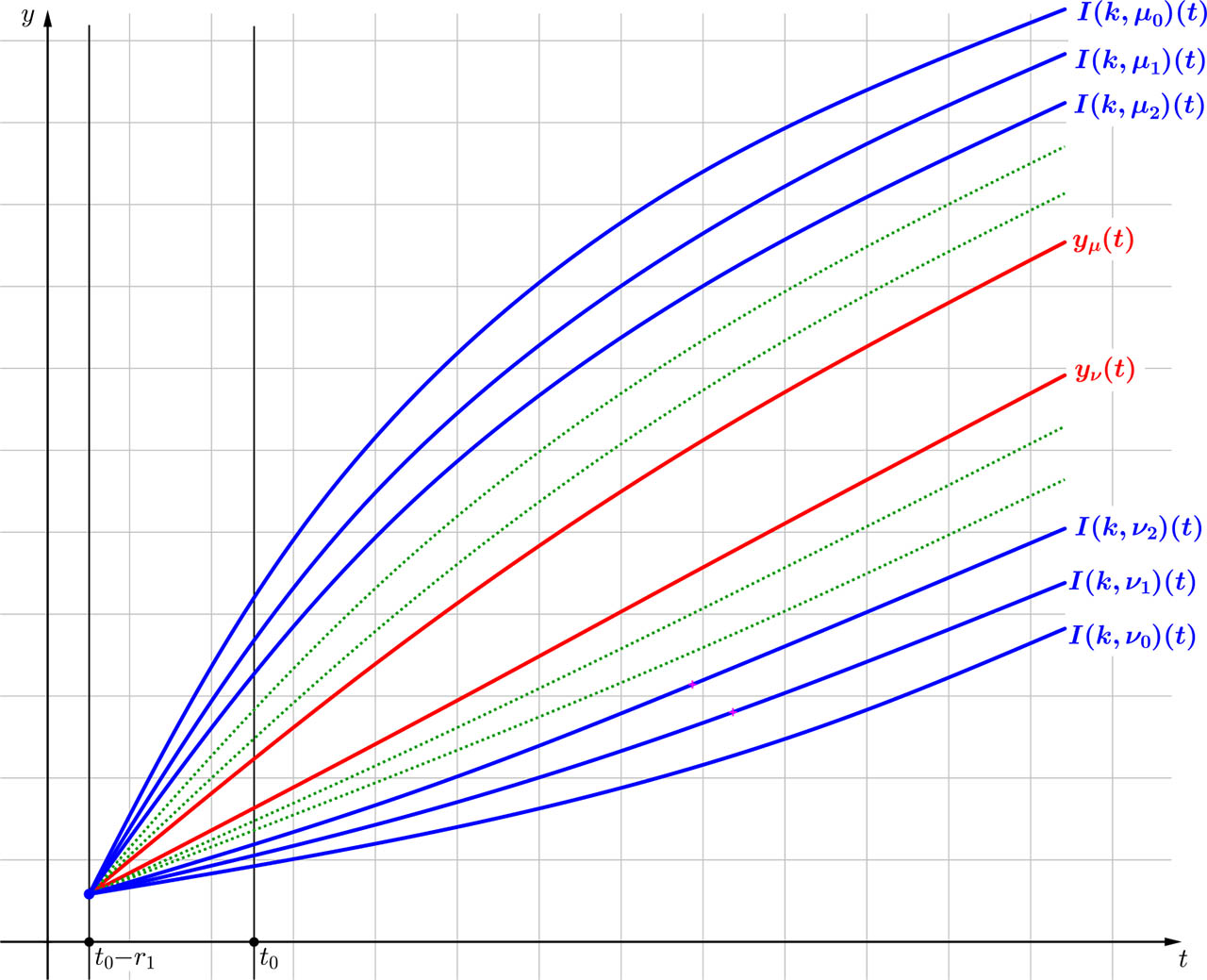
The theorem applied to monotone iterative sequences. Now, we are ready to apply Theorem 7.A in [33, p. 283]. The function ν₀(t) satisfies ν₀(t) ≤ (Gν₀)(t) and is a subsolution of the operator G whereas μ₀(t), satisfying μ₀(t) ≥ (Gμ₀)(t), is its supersolution. Since all the hypotheses of the theorem hold, the iterative sequence {νi(t)}i=0∞ converges to the smallest fixed point ν(t) of G in [ν₀(t), μ₀(t)], whereas the iterative sequence {μi(t)}i=0∞ converges to the greatest fixed point μ(t), of G in [ν₀(t), μ₀(t)]. Therefore, (a visualization is in Figure 1)

ℒ(t)=ν0(t)⩽νi(t)⩽ν(t)⩽μ(t)⩽μi(t)⩽μ0(t)=ℛ(t), t∈J−1+, i=1,… .

The functions λ(t) := ν(t) ∈ L, λ(t) := μ(t) ∈ L are fixed points of the operator G and, because of the relation between G and T defined by (2.11) and (2.2), functions y(t) = y_ν(t) = I(k, ν)(t), y(t) = y_μ(t) = I(k, μ)(t) are solutions of the equation (2.3) as well. A visualization is in Figure 2. The remaining properties formulated in the theorem are immediate consequences of the properties of the iterative process.

Fig. 2

To the proof of Theorem 1.

Example 1

Let us prove the existence of a right semi-global positive solution to the nonlinear equation

(2.21) y˙(t)=(sint)2e−ty(t−1)y(t+1).

We have n = 1, r₁ = r₂ = 1. Let t₀ = 1. Then, 𝒥⁺ = [1, ∞) , J−1+:=[0,∞) and equation (2.3) takes the form

(2.22) λ(t)=(Tλ)(t):=k(sint)2e−t(exp∫0t−1λ(s)ds)(exp∫tt+1λ(s)ds), t∈J+.

Apply now Theorem 1. Let k ∈ (0, 1] be fixed. It is easy to see that condition (i) is fulfilled. Functions ℒ, ℛ: J−1+→ℝn defined as ℒ := 0, ℛ := k satisfy condition (ii) since

0=ℒ(t)⩽(Tℒ)(t)=k(sint)2e−t, t∈J+

and

k=ℛ(t)⩾(Tℛ)(t)=k(sint)2et(k−1), t∈J+.

Condition (iii) holds obviously if φ(t) := 0, t ∈ [0, 1]. Condition (iv) holds as well since, as follows from (2.22), for any two continuous functions λ, μ : J−1+→ℝ1 , the inequality λ(t) ≤ μ(t), t∈J−1+ implies inequality (2.6). All the hypotheses of Theorem 1 hold and, by (2.8) with i = j = 0, there exists a right semi-global solution y : J−1+→ℝ1 of (2.21) satisfying y(0) = k and

(2.23) I(k,ℒ)(t)=k⩽y(t)⩽kekt=I(k,ℛ)(t), t∈[0,∞).

If we set i = j = 1, then

ν1(t)={(Tν0)(t)=k(sint)2e−t,t∈[1,∞),(Tν0)(0)=k(sin1)2e−1,t∈[0,1),

μ1(t)={(Tμ0)(t)=k(sint)2et(k−1),t∈[1,∞),(Tμ0)(0)=k(sin1)2ek−1,t∈[0,1)

and inequality (2.23) can be improved to

(2.24) kexp(∫0tν1(s)ds)⩽y(t)⩽kexp(∫0tμ1(s)ds), t∈[0,∞).

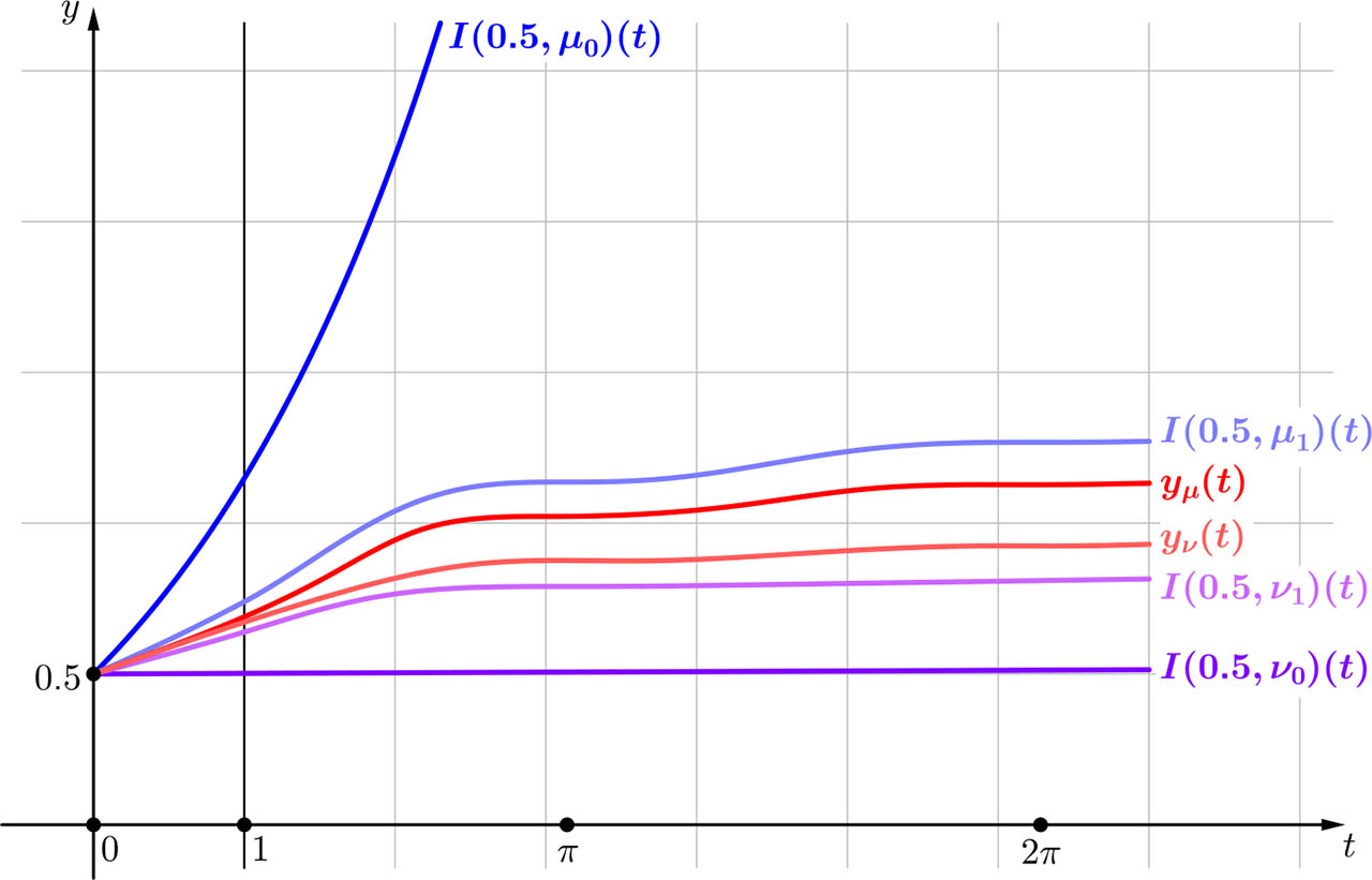
Both integrals can be easily computed, but the results are too cumbersome to write down. Rather, we refer to to Figure 3 which, for k = 0.5, depicts the “starting” functions (a subsolution and a supersolution) ν₀ = ℒ, μ₀ = ℛ, their images(by operator T) ν₁, μ₁, and possible limits ν, μ. Figure 4 shows the behaviour of I(0.5, ν₀)(t), I(0.5, ν₁)(t), I(0.5, μ₀)(t), I(0.5, μ₁)(t) and possible solutions y_ν(t), y_μ(t). It can be seen that, for the case considered, the function I(0.5, μ₁)(t) (i.e. the right-hand side of (2.24)) substantially improves the right-hand side of (2.23) given by I(0.5, μ₀)(t).

Fig. 3

To Example 1.

Fig. 4

To Example 1.

Example 2

Let n = 2. Consider a non-linear system

(2.25) y˙1(t)=e−t−2y1(t)y2(t+1),

(2.26) y˙2(t)=e−t−2y1(t−1)y2(t).

Let t₀ = 1. We have r₁ = r₂ = 1, t₀ = 1, 𝒥⁺ = [1, ∞) and J−1+:=[0,∞) . Set k₁ = k₂ = 1. The operator equation (2.3) reduces to

(2.27) λ1(t)=(T1λ)(t):=e−t−2exp(∫0t+1λ2(s)ds),

(2.28) λ2(t)=(T2λ)(t):=e−t−2exp(∫0t−1λ1(s)ds).

Let ℒ_i(t) = 0, ℛ_i(t) = 1, i = 1, 2. Condition (i) of Theorem 1 is obviously fulfilled and we omit its verification. Let us show that condition (ii) holds. The first inequality in (2.5), L(t) ≤ (Tℒ)(t), is fulfilled because the right-hand sides of inequalities (2.27), (2.28) are positive. The second inequality, ℛ(t) ≥ (Tℛ)(t) in (2.5) holds as well, as given by the below estimates

(T1ℛ)(t)=e−t−2exp(∫0t+11 ds)=e−1<1=ℛ1(t),(T2ℛ)(t)=e−t−2exp(∫0t−11 ds)=e−3<1=ℛ2(t).

For the choice φ(t) ≡ 0, t ∈ [0, 1], the condition (iii) holds as a consequence of (ii) and the fact that functions ℒ, ℛ are constant. Inequality (2.7) in condition (iv) holds as well, this is because t ≥ t₀ = 1, as can be easily derived from the right-hand sides of (2.27), (2.28) defining the operator (Tλ)(t). By Theorem 1 (where i = j = 0 in (2.8)), there exists a right semi-global solution y = (y₁, y₂) of (2.25), (2.26) on J−1+:=[0,∞) satisfying y_i(0) = 1, i = 1, 2 and

1⩽yi(t)⩽et, t>0, i=1,2.

2.1 Right semi-global solutions in a linear case

In this section we will consider a scalar linear equation, as a particular case of equation (1.1),

(2.29) y˙(t)=f(t,yt,yt):=−c(t)y(t−τ(t))+d(t)y(t+σ(t))

where the functions c, d : 𝒥⁺ → [0, ∞), τ : 𝒥⁺ → [0, r₁] and σ : 𝒥⁺ → [0, r₂] are Lipschitz continuous.

Theorem 2

Consider bounded continuous functions ℒ, ℛ: J−1+→ℝ , ℒ(t) ≤ ℛ(t), t∈J−1+ and a Lipschitz continuous function φ : [t₀ − r₁, t₀] → ℝ satisfying φ(t₀) = 0. Moreover, let

(2.30) ℒ(t)⩽−c(t)exp(∫tt−τ(t)ℒ(s) ds)+d(t)exp(∫tt+σ(t)ℒ(s) ds),

(2.31) ℛ(t)⩾−c(t)exp(∫tt−τ(t)ℛ(s) ds)+d(t)exp(∫tt+σ(t)ℛ(s) ds)

on 𝒥⁺ and

(2.32) ℒ(t)⩽−c(t0)exp(∫t0t0−τ(t0)ℒ(s) ds)+d(t0)exp(∫t0t0+σ(t0)ℒ(s) ds)+φ(t),

(2.33) ℛ(t)⩾−c(t0)exp(∫t0t0−τ(t0)ℛ(s) ds)+d(t0)exp(∫t0t0+σ(t0)ℛ(s) ds)+φ(t)

on [t₀ − r₁, t₀]. Then, there exists a right semi-global solution y(t) of (2.29) on J−1+ such that y(t₀ − r₁) = 1 and, for arbitrary indexes i ≥ 0, j ≥ 0,

(2.34) exp( ∫t0−r1tνi(s) ds)⩽ y(t)⩽exp( ∫t0−r1tμj(s) ds), t∈J−1+

where ν_i(t) ≤ ν_i₊₁(t), μ_j₊₁(t) ≤ μ_j(t), ν_i(t) ≤ μ_j(t), ν₀(t) := ℒ(t), μ₀(t) := ℛ(t), t∈J−1+ , and, for i > 0, j > 0,

νi(t):={−c(t)exp(∫tt−τ(t)νi−1(s) ds)+d(t)exp(∫tt+σ(t)νi−1(s) ds), t∈[t0,∞), νi(t0), t∈[t0−r1,t0),μj(t):={−c(t)exp(∫tt−τ(t)μj−1(s) ds)+d(t)exp(∫tt+σ(t)μj−1(s) ds), t∈[t0,∞), μj(t0), t∈[t0−r1,t0).

Moreover, there exist continuous limits ν(t) = lim_i→∞ ν_i(t), μ(t) = lim_j→∞ μ_j(t), ν(t) ≤ μ(t), t∈J−1+ defining right semi-global solutions y_ν, y_μ: J−1+→ℝ of (2.29) and satisfying y_ν(t₀ − r₁) = y_μ(t₀ − r₁) = 1, by formulas

yν(t)=exp( ∫t0−r1tν(s) ds), yμ(t)=exp( ∫t0−r1tμ(s) ds), t∈J−1+

and, for arbitrary indexes i ≥ 0, j ≥ 0,

exp( ∫t0−r1tνi(s) ds)⩽yν(t)⩽yμ(t)⩽exp( ∫t0−r1tμj(s) ds), t∈J−1+,

Proof

Let us apply Theorem 1 to prove the existence of a solution to (2.29). Set k = 1. Then,

I(k,λ)(t)=exp( ∫t0−r1tλ(s) ds).

First, we verify condition (i). In the considered case,

(2.35) (Tλ)(t):=−c(t)exp(∫tt−τ(t)λ(s) ds)+d(t)exp(∫tt+σ(t)λ(s) ds).

Let us estimate the left-hand side of (2.4). We derive

For |λ| ≤ M, τ(t) ≤ r₁ and σ(t) ≤ r₂,

(2.37) exp(∫tt−τ(t)λ(s) ds)⩽exp(Mr1), exp(∫tt+σ(t)λ(s) ds)⩽exp(Mr2).

Because of the Lipschitz continuity of functions c and d, there exist constants L_c and L_d such that |c(t) − c(t^′)| ≤ L_c |t − t^′|, |d(t) − d(t^′)| ≤ L_c |t − t^′| and, by Lagrange mean value theorem,

|exp(∫tt−τ(t)λ(s) ds)−exp(∫t′t′−τ(t′)λ(s) ds)|=ea|∫tt−τ(t)λ(s) ds−∫t′t′−τ(t′)λ(s) ds|

for some a between ∫tt−τ(t)λ(s) ds and ∫t′t′−τ(t′)λ(s) ds . Moreover, exp(a) ≤ exp(Mr₁). Using the Lipschitz continuity of τ, i.e. |τ(t) − τ(t^′)|. ≤ L_τ|t − t^′|, we obtain

|∫tt−τ(t)λ(s) ds−∫t′t′−τ(t′)λ(s) ds|=|∫tt′λ(s) ds+∫t′−τ(t′)t−τ(t)λ(s) ds| ⩽M|t−t′|+M|t−t′−τ(t)+τ(t′)|⩽2M|t−t′|+MLτ|t−t′|.

Consequently,

(2.38) |exp(∫tt−τ(t)λ(s) ds)−exp(∫t′t′−τ(t′)λ(s) ds)|⩽eMr1M(2+Lτ)|t−t′|.

In much the same way as above, using Lagrange mean value theorem and Lipschitz continuity of σ with Lipschitz constant L_σ,

(2.39) |exp(∫tt+σ(t)λ(s) ds)−exp(∫t′t′+σ(t′)λ(s) ds)|⩽eMr2M(2+Lσ)|t−t′|.

Summarizing the estimates (2.36)–(2.39), we see that condition (i) holds if

K:=eMr1(Lc+MMc(2+Lτ))+eMr2(Ld+MMd(2+Lσ)),

where M_c and M_d are upper bounds for c and d on [t₀, θ].

Second, condition (ii) is a direct consequence of inequalities (2.30), (2.31) and (iii) holds due to (2.32), (2.33). Finally, it is easy to see that (iv) holds, i.e., for any two continuous functions λ*, μ* : J−1+→ℝ such that λ*(t) ≤ μ*(t), t∈J−1+ , the inequality (2.7) holds because of the properties of c, d, τ and σ. All the hypotheses of Theorem 1 are fulfilled, a solution of (2.29) on J−1+ exists and the inequality (2.34) holds because of (2.8). The remaining properties, too, follow immediately from the conclusion of Theorem 1.

Example 3

In this example we show that whether inequalities (2.32), (2.33) hold may depend a great deal on a suitable choice of the function φ in Theorem 2. We will prove the existence of right semi-global solutions to a scalar equation

(2.40) y˙(t)=−e 8t3y(t−1)+1e(1+18t2)y(t+1),

which is a (2.29)-type equation for τ(t) = 1, σ(t) = 1, c(t) = e(8t³)⁻¹ and d(t) = e⁻¹(1 + 1/(8t²))⁻¹. We have r₁ = r₂ = 1. Assume that t₀ is sufficiently large. Applying this tacitly below, let us further assume that the expressions in consideration are well-defined and the asymptotic computations are correct. We will show that there exists a positive solution to (2.40) on J−1+ and describe its asymptotic behaviour. Define an auxiliary function

λδ(t)=1+12t+δ2tlnt

where δ ∈ ℝ. Let numbers δ₁ and δ₂ be chosen in such a way that inequality (2.30) with ℒ := λ_δ₁ and inequality (2.31) with ℛ := λ_δ₂ hold. Omitting long computations, the following asymptotic decompositions can be derived where the symbol o stands for the Landau order symbol small “o”. This is possible by using asymptotic representations for functions (arising when integrals are computed) of the type (t − p)^q, ln^q(t − p) where t → ∞ and p, q ∈ ℝ, we refer, e.g., to formulas in [9], Lemmas 4.1, 4.2. The right-hand side of (2.30) equals

λδ1(t)+δ1(δ1−2)8t2(lnt)2+o(1t3)

and (2.30) will hold if

0<δ1(δ1−2)8t2(lnt)2+o(1t3)

that is, if δ₁ < 0 or if δ₁ > 2. Similarly, for the right-hand side of (2.31), we get

λδ2(t)+δ2(δ2−2)8t2(lnt)2+o(1t3)

and (2.31) will hold if

0>δ2(δ2−2)8t2(lnt)2+o(1t3)

that is, if δ₂ ∈ (0, 2). Fix a δ₁ < 0 and δ₂ ∈ (0, 2), then ℒ < ℛ and inequalities (2.30), (2.31) hold. Let φ(t) := ℛ(t) − ℛ(t₀) = λ_δ₂ (t) − λ_δ₂ (t₀), t ∈ [t₀ − 1, t₀]. Then, after asymptotic computations, inequality (2.32) can be simplified to

(δ1−δ2)[12tlnt−12t0lnt0]⩽δ1(δ1−2)8t02(lnt0)2+o(1t03).

This inequality holds because its left-hand side is non-positive and right-hand side is positive. Inequality (2.33) holds as well because it is a consequence of (2.31) if t = t₀. All the hypotheses of Theorem 2 hold and, by inequality (2.34) where i = j = 0, there exists a solution y(t) of equation (2.40) on J−1+ such that y(t₀ − 1) = 1 and

(2.41) ett(lnt)δ1et0−1(t0−1)(ln(t0−1))δ1⩽y(t)⩽ett(lnt)δ2et0−1(t0−1)(ln(t0−1))δ2

where t ∈ [t₀ − 1, ∞). Inequalities (2.41) give a fitting description of the asymptotic behaviour of y(t). Note that we have obtained it thanks to an appropriate choice of the function φ.

We will show why the choice of φ(t) ≡ 0, t ∈ [t₀ − 1, t₀] is unsuitable here. The reason is that, then, (2.32) implies that, for all suficiently large values of t,

12t+δ12tlnt⩽12t0+δ12t0lnt0+δ1(δ1−2)8t02(lnt0)2+o(1t03).

In the above inequality, set t = t₀ − 1 as the admissible value rewriting it in an equivalent form

1+δ1(t0lnt0−(t0−1)ln(t0−1))ln(t0−1)lnt0⩽δ1(δ1−2)(t0−1)4t0(lnt0)2+o(1t0).

Letting t₀ → ∞ we easily conclude that the limits of all terms are zeros, except for the first one, and that the inequality takes the form 1 ≤ 0. So, such a choice of φ is impossible.

2.2 On the convergence of iterative process

Let us take an example of the autonomous equation (2.29),

(2.42) y˙(t)=−e0.02y(t−0.01)+3e−0.02y(t+0.01),

with a solution y(t) = exp(2t) to illustrate the iterative process. Here c(t) = exp(0.02), d(t) = 3 exp(−0.02) and τ(t) = r₁ = 0.01, σ(t) = r₂ = 0.01. For ℒ(t) = μ₀(t) = 1, ℛ(t) = ν₀(t) = 3, φ(t) = 0, all the hypotheses of Theorem 2 are fulfilled (the value t₀ can be arbitrary). The operator T defined by (2.35), where λ is assumed a constant function, reduces to

(Tλ)(t):=−e0.02−0.01λ+3e−0.02+0.01λ

and

μi=(Tμi−1), νi=(Tνi−1)(t), i⩾1.

One of the fixed points of T is the value λ = 2. Computation in Matlab for i = 1, . . . , 7 reveals that the above sequences converge very fast to this limit value, as shown in Table 1. From formula (2.34) with t₀ = 1, we conclude that there exists a solution y = y(t) of equation (2.42) such that y(0) = 1 and e^{ν_i t} ≤ y(t) ≤ e^{μ_i t}, i = 0, 1, . . . , t ∈ [0, ∞).

Table 1

Convergence of iterative sequences.

i = 0	ν₀ = 1	μ₀ = 3
i = 1	ν₁ = 1.960099334	μ₁ = 2.040100667
i = 2	ν₂ = 1.998404132	μ₂ = 2.001604188
i = 3	ν₃ = 1.999936166	μ₃ = 2.000064168
i = 4	ν₄ = 1.999997447	μ₄ = 2.000002567
i = 5	ν₅ = 1.999999898	μ₅ = 2.000000103
i = 6	ν₆ = 1.999999996	μ₆ = 2.000000004
i = 7	ν₇ = 1.999999999	μ₇ = 2.000000000
. . .	. . .	. . .
i = ∞	ν = 2	μ = 2

3 Left Semi-Global Solutions

The goal of this section is to prove the existence of left semi-global solutions to mixed-type system (1.1). Theorem 3 below is a modification of Theorem 1 for the existence of a left semi-global solution of (1.1). A linear particular case is considered in section 3.1 as well.

Define a mapping

I*:ℝ>0n×C(J+1−,ℝn)→C(J+1−,ℝn)

where I*(k,λ)=(I1*(k,λ),I2*(k,λ),…,In*(k,λ)), k∈ℝ>0n is a constant vector, λ∈C(J+1−,ℝn) is a vector-function and

Ii*(k,λ)(t):=kiexp(∫tt0+r2λi(s) ds), i=1,…,n, t∈J+1−.

We are looking for a solution of system (1.1) in the form y(t) = I*(k, λ)(t), t∈J+1− with suitable k and λ. This leads to the operator equation

(3.1) λ(t)=(T*λ)(t):=−f(t,I*(k,λ)t,I*(k,λ)t)(diag(I*(k,λ)(t)))−1, t∈J−

where T*:C(J+1−,ℝn)→C(J−,ℝn) .

Theorem 3

Let us assume that k∈ℝ>0n and that the following holds:

For any M ≥ 0, θ < t₀, there exists a constant K, such that, for all t, t^′ ∈ [θ, t₀] and for any continuous function λ : J+1−→ℝn with |λ| ≤ M,
|(T*λ)(t)−(T*λ)(t′)|⩽K|t−t′|.
There exist bounded continuous functions ℒ, ℛ: J+1−→ℝn satisfying ℒ(t) ≤ ℛ(t), t∈J+1− and
(3.2) ℒ(t)⩽(T*ℒ)(t), ℛ(t)⩾(T*ℛ)(t), t∈J−.
There exists a Lipschitz continuous function φ : [t₀, t₀ + r₂] → ℝⁿ satisfying φ(t₀) = 0 and
ℒ(t)⩽(T*ℒ)(t0)+φ(t), ℛ(t)⩾(T*ℛ)(t0)+φ(t), t∈[t0,t0+r2].
For any locally integrable functions λ*, μ* : J+1−→ℝn , the inequality λ*(t) ≤ μ*(t), t∈J+1− implies
(3.3) (T*λ*)(t)⩽(T*μ*)(t), t∈J−.

Then, there exists a left semi-global solution y : J+1−→ℝn of (1.1) satisfying y(t₀ + r₂) = k and such that, for arbitrary indices i ≥ 0, j ≥ 0,

(3.4) I*(k,νi)(t)⩽y(t)⩽I*(k,μj)(t), t∈J+1−

where ν_i(t) ≤ ν_i₊₁(t), μ_j₊₁(t) ≤ μ_j(t), ν_i(t) ≤ μ_j(t), ν₀(t) := ℒ(t), μ₀(t) := ℛ(t), t∈J+1− , and, for i > 0, j > 0,

νi(t):={(T*νi−1)(t),t∈(−∞,t0],(T*νi−1)(t0)+φ(t),t∈(t0,t0+r2],μj(t):={(T*μj−1)(t),t∈(−∞,t0],(T*μj−1)(t0)+φ(t),t∈(t0,t0+r2].

Moreover, there exist continuous limits

ν(t)=limi→∞νi(t), μ(t)=limj→∞μj(t), ν(t)⩽μ(t), t∈J+1−,

defining left semi-global solutions y_ν(t) = I*(k, ν)(t), y_μ(t) = I*(k, μ)(t), y_ν, y_μ : J+1−→ℝn of (1.1), satisfying y_ν(t₀ − r₁) = y_μ(t₀ − r₁) = k and inequalities

I*(k,νi)(t)⩽yν(t)⩽yμ(t)⩽I*(k,μj)(t), t∈J+1−

where i ≥ 0, j ≥ 0 are arbitrary.

Proof

The proof is similar to the proof of Theorem 1 with minor changes. We search for the solution λ∈C(J+1−,ℝ) of (3.1) such that ℒ(t) ≤ λ(t) ≤ ℛ(t) for t∈ J+1− . An auxiliary operator G* : L → L := C(J+1−,ℝn) , analogous to the operator G, is defined by the formula

(G*λ)(t)={(T*λ)(t),t∈(−∞,t0],(T*λ)(t0)+φ(t),t∈(t0,t0+r2].

The remaining parts of the proof can be modified easily.

Example 4

Let n = 1 and let (1.1) be reduced to a nonlinear equation

(3.5) y˙(t)=−(cost)2e2ty2(t)y(t−sint).

Set t₀ = −1. Then, since r₁ = r₂ = 1, we have J⁻ = (−∞, −1] and J+1−=(−∞,0] . This equation changes its type, being delayed or advanced if sin t > 0 or sin t < 0, respectively. By Theorem 3, we prove that there exist nontrivial left semi-global solutions to equation (3.5). Let 0 < k ≤ e^−1/2. The operator equation (3.1) has the form

λ(t)=(T*λ)(t):=k2(cost)2e2t(exp∫t0λ(s)ds)(exp∫t−sint0λ(s)ds), t∈J−.

Condition (i) can be simply verified and we omit the technical details. Condition (ii) with inequalities (3.2) hold for ℒ, ℛ: J+1−→ℝn defined as ℒ := 0, ℛ := 1 because

0=ℒ(t)⩽(T*ℒ)(t)=k2(cost)2e2t, t∈J−

and

1=ℛ(t)⩾(T*ℛ)(t)=k2(cost)2esint, t∈J−.

The choice φ(t) := 0, t ∈ [−1, 0] implies that condition (iii) holds. Moreover, for any locally integrable functions λ, μ : J+1−→ℝ1 such that λ(t) ≤ μ(t), t∈J+1− , inequality (3.3) holds because the operator T* is increasing and (iv) holds. By Theorem 3, for every admissible fixed k, there exists a left semi-global solution y : J+1−→ℝ of (3.5) satisfying y(0) = k and (3.4), where i = j = 0, that is,

I*(k,ℒ)(t)=k⩽y(t)⩽ke−t=I*(k,ℛ)(t), t∈(−∞,0].

3.1 Left semi-global solutions in a linear case

In this section, linear equation (2.29) is considered assuming that functions c, d : 𝒥⁻ → [0, ∞), τ : 𝒥⁻ → [0, r₁] and σ : 𝒥⁻ → [0, r₂] are Lipschitz continuous.

Theorem 4

Let there be bounded continuous functions ℒ, ℛ: J+1−→ℝ , ℒ(t) ≤ ℛ(t), t∈J+1− and a Lipschitz continuous function φ : [t₀, t₀ + r₂] → ℝ satisfying φ(t₀) = 0. Moreover, let

(3.6) ℒ(t)⩽c(t)exp( ∫t−τ(t)tℒ(s) ds)−d(t)exp( ∫t+σ(t)tℒ(s) ds),

(3.7) ℛ(t)⩾c(t)exp( ∫t−τ(t)tℛ(s) ds)−d(t)exp( ∫t+σ(t)tℛ(s) ds)

on 𝒥⁻ and

(3.8) ℒ(t)⩽c(t0)exp( ∫t0−τ(t0)t0ℒ(s) ds)−d(t0)exp( ∫t0+σ(t0)t0ℒ(s) ds)+φ(t),

(3.9) ℛ(t)⩾c(t0)exp( ∫t0−τ(t0)t0ℛ(s) ds)−d(t0)exp( ∫t0+σ(t0)t0ℛ(s) ds)+φ(t)

on [t₀, t₀ + r₂]. Then, there exists a left semi-global solution y(t) of (2.29) on J+1− such that y(t₀ + r₂) = 1 and, for arbitrary indexes i ≥ 0, j ≥ 0,

(3.10) exp(∫tt0+r2νi(s) ds)⩽y(t)⩽exp(∫tt0+r2μj(s) ds), t∈J+1−

where ν_i(t) ≤ ν_i₊₁(t), μ_j₊₁(t) ≤ μ_j(t), ν_i(t) ≤ μ_j(t), ν₀(t) := ℒ(t), μ₀(t) := ℛ(t), t∈J+1− , and, for i > 0, j > 0,

νi(t):={c(t)exp( ∫t−τ(t)tνi−1(s) ds)−d(t)exp( ∫t+σ(t)tνi−1(s) ds), t∈(−∞,t0],νi(t0), t∈(t0,t0+r2],μj(t):={c(t)exp( ∫t−τ(t)tμj−1(s) ds)−d(t)exp( ∫t+σ(t)tμj−1(s) ds), t∈(−∞,t0],μj(t0), t∈(t0,t0+r2].

Moreover, there exist continuous limits ν(t) = lim_i→∞ ν_i(t), μ(t) = lim_j→∞ μ_j(t), ν(t) ≤ μ(t), t∈J+1− , defining left semi-global solutions y_ν, y_μ : J+1−→ℝ of (2.29) satisfying y_ν(t₀ + r₂) = y_μ(t₀ + r₂) = 1, by the formulas

yν(t)=exp(∫tt0+r2ν(s) ds), yμ(t)=exp(∫tt0+r2μ(s) ds), t∈J+1−

and, for arbitrary indexes i ≥ 0, j ≥ 0,

exp(∫tt0+r2νi(s) ds)⩽yν(t)⩽yμ(t)⩽exp(∫tt0+r2μj(s) ds), t∈J+1−.

Proof

The proof is omitted since it is similar to the proof of Theorem 2 and uses the conclusion of Theorem 3.

Example 5

Consider the existence of left semi-global solutions to the scalar linear equation

(3.11) y˙(t)=−ety(t−1)+e−1(sint)2y(t+1),

which is a particular case of equation (2.29), where τ(t) = 1, σ(t) = 1, c(t) = e^t, d(t) = e⁻¹(sin t)². We have r₁ = r₂ = 1. Let t₀ = −2. Then, 𝒥⁻ = (−∞, −2] and J+1−=(−∞,−1] . Now, verify the hypotheses of Theorem 4 assuming ℒ(t) = −1, ℛ(t) = 1, t ∈ (−∞, −1], and φ ≡ 0, t ∈ [−2, −1]. The resulting estimate of the right-hand side of (3.6) is

ete−1−e−1(sint)2e>−(sint)2⩾−1=ℒ(t), t∈J−

and (3.6) holds. Estimating the right-hand side of (3.7) leads to

ete−e−1(sint)2e−1⩽et+1⩽e−1<1=ℛ(t), t∈J−

and (3.7) holds as well. Similarly, it can be verified that inequalities (3.8), (3.9) hold (because ℒ(t), ℛ(t) are constants). All the hypotheses of Theorem 4 hold and, by inequality (3.10) with i = j = 0, there exists a solution y(t) of equation (3.11) on J+1− such that y(−1) = 1 and

et+1⩽y(t)⩽e−t−1, t∈(−∞,−1].

4 Semi-Global Solutions in Non-Iterative Case

Carefully tracing the proof of Theorem 1, we can derive a theorem on the existence of semi-global solutions of classes of equations without applying the monotone iterative method. In this case, we will get upper and below estimates of semi-global solutions without the possibility of improving them in an iterative process, that is, without using functions of the type ν_i(t), μ_i(t), i = 0, 1, . . . .

Theorem 5

Let us assume that k∈ℝ>0n . Let the hypotheses (i), (ii) and (iii) of Theorem 1 hold. If, moreover, for any locally integrable function λ : J−1+→ℝn , the inequality

ℒ(t)⩽λ(t)⩽ℛ(t), t∈J−1+

implies

(4.1) (Tℒ)(t)⩽(Tλ)(t)⩽(Tℛ)(t), t∈J+,

then there exists a right semi-global solution y : J−1+→ℝn of (1.1) satisfying y(t₀ − r₁) = k and

I(k,ℒ)(t)⩽y(t)⩽I(k,ℛ)(t), t∈J−1+.

Proof

The proof can be done along the same lines as the proof of Theorem 1 with the following modification. From the above proof, we delete the parts Monotone iterative sequences and The theorem applied to monotone iterative methods. Since the operator G is compact and the property (4.1) is assumed, by Schauder-Tychonoff fixed-point theorem, there exists a fixed point of G and the relation between G and T defined by (2.11) implies that it is a solution of the equation (2.3).

The following theorem can be proved in much the same way based on Theorem 3.

Theorem 6

Let us assume that k∈ℝ>0n . Let the hypotheses (i), (ii) and (iii) of Theorem 3 hold. If, moreover, for any locally integrable function λ* : J+−1→ℝn , the inequality

ℒ(t)⩽λ*(t)⩽ℛ(t), t∈J+1−

implies

(T*ℒ)(t)⩽(T*λ*)(t)⩽(T*ℛ)(t), t∈J−,

then there exists a left semi-global solution y : J+1−→ℝn of (1.1) satisfying y(t₀ + r₂) = k and

I*(k,ℒ)(t)⩽y(t)⩽I*(k,ℛ)(t), t∈J+1−.

Remark 1

For the case of a linear equation (2.29), Theorems 2 and 4 use simplified hypotheses of Theorems 1 and 3. Also, for such a linear equation, the hypotheses of Theorems 5 and 6 are equivalent with those of Theorems 2 and 4 and so the linear case need not be considered separately.

5 Global Solutions

This section is concerned with the existence of global solutions on the entire ℝ. The general case is treated in section 5.1 using the iterative method, and a particular linear case in section 5.2. This problem without the iterative method applied is discussed in section 5.3.

Assume the existence of bounded continuous functions ℒ, ℛ: ℝ → ℝⁿ which satisfy

(5.1) ℒ(t)⩽ℛ(t), t∈ℝ.

By Ω we denote the set of the functions λ ∈ C(ℝ, ℝⁿ) with the property ℒ(t) ≤ λ(t) ≤ ℛ(t), t ∈ ℝ, that is,

Ω:={λ∈C(ℝ,ℝn):ℒ(t)⩽λ(t)⩽ℛ(t)}.

Define a mapping

I**:ℝ>0n×ℝ×C(ℝ,ℝn)→C(ℝ,ℝn)

where I**(k,t∗,λ)=(I1**(k,t∗,λ),I2**(k,t∗,λ),…,In**(k,t∗,λ)) , k∈ℝ>0n is a constant vector, λ ∈ C (ℝ, ℝⁿ) is a vector-function, t_* ∈ ℝ is fixed, and

(5.2) Ii**(k,t∗,λ)(t):=kiexp(∫t∗tλi(s) ds), i=1,…,n, t∈ℝ.

Let us look for a solution of equation (1.1) in an exponential form

(5.3) y(t)=I**(k,t∗,λ)(t)

with suitable k∈ℝ>0n , t_* ∈ ℝ and λ ∈ C (ℝ, ℝⁿ). This leads to the operator equation

(5.4) λ(t)=(T**λ)(t):=f(t,I**(k,t∗,λ)t,I**(k,t∗,λ)t)(diag(I**(k,t∗,λ)(t)))−1

where t ∈ ℝ and T** : C(ℝ, ℝⁿ) → C(ℝ, ℝⁿ).

5.1 Global solutions found by iterative monotone method

With several modifications, the monotone iterative method used in the proof of Theorem 1, can be employed to prove the existence of global solutions as well. This is described by the below theorem.

Theorem 7

Let k∈ℝ>0n , t_* ∈ ℝ and let ℒ, ℛ: ℝ → ℝⁿ be bounded continuous functions, satisfying (5.1). Let, moreover, the following hold.

For any fixed a, b ∈ ℝ, a < b, there exists a constant K such that, for any function λ ∈ Ω,
|(T**λ)(t)−(T**λ)(t′)|⩽K|t−t′|
for arbitrary t, t^′ ∈ [a, b].
ℒ(t) ≤ (T**ℒ)(t), ℛ(t) ≥ (T**ℛ)(t), t ∈ ℝ.
For any λ*, μ* ∈ Ω, the inequality
ℒ(t)⩽λ*(t)⩽μ*(t)⩽ℛ(t), t∈ℝ
implies
(T**ℒ)(t)⩽(T**λ*)(t)⩽(T**μ*)(t)⩽(T**ℛ)(t), t∈ℝ.

Then, there exists a global solution y : ℝ → ℝⁿ of (1.1) satisfying y(t_*) = k and, for arbitrary indexes i ≥ 0, j ≥ 0,

(5.5) I**(k,t∗,νi)(t)⩽y(t)⩽I**(k,t∗,μj)(t) for t*<t,

(5.6) I**(k,t∗,μj)(t)⩽y(t)⩽I**(k,t∗,νi)(t) for t*>t,

where ν_i(t) ≤ ν_i₊₁(t), μ_j₊₁(t) ≤ μ_j(t), ν_i(t) ≤ μ_j(t), ν₀(t) := ℒ(t), μ₀(t) := ℛ(t), t∈J−1+ , and, for i > 0, j > 0,

(5.7) νi(t):=(T**νi−1)(t), μj(t):=(T**μj−1)(t), t∈ℝ.

Moreover, there exist continuous limits

(5.8) ν(t)=limi→∞νi(t), μ(t)=limj→∞μj(t), ν(t)⩽μ(t), t∈ℝ,

defining global solutions by the formulas y_ν(t) = I(k, ν)(t), y_μ(t) = I(k, μ)(t), t ∈ ℝ satisfying y_ν(t_*) = y_μ(t_*) = k and inequalities

I**(k,t∗,νi)(t)⩽yν(t)⩽yμ(t)⩽I**(k,t∗,μj)(t) for t*<t,I**(k,t∗,μj)(t)⩽yμ(t)⩽yν(t)⩽I**(k,t∗,νi)(t) for t*>t,

where i ≥ 0, j ≥ 0 are arbitrary.

Proof

As mentioned above, the proof is a variant of the proof of Theorem 1 with the following changes. Instead of the space L, the Banach space L = C(ℝ, ℝⁿ) is used of bounded continuous functions from ℝ into ℝⁿ and the closed, normal order cone is defined as K:=C(ℝ,ℝ⩾0n) . The operator T** : L → L is used instead of the previous operator G. The monotone iterative sequences are constructed in much the same way by formulas (5.7) and inequalities

ℒ(t)=ν0(t)⩽ν1(t)⩽⋯⩽νi(t)⩽⋯⩽μi(t)⩽⋯⩽μ1(t)⩽μ0(t)=ℛ(t)

where i = 0, 1, . . . , and t ∈ ℝ, similar to (2.16) are guaranteed to hold by (ii) and (iii). Similarly, with (i), the compactness of T** can be proved. Finally, Theorem 7.A in [33, p. 283] on monotone iterative methods can be applied to confirm the existence of limit functions (5.8) with the desired properties.

Example 6

Let n = 1, t_* ∈ ℝ and k = 1 be fixed. We will use Theorem 7 to prove the existence of a positive global solution to the linear equation

(5.9) y˙(t)=(sint)y(t+εsint)

where t ∈ ℝ, r₁ = r₂ = ε and ε is a fixed constant satisfying 0 < ε ≤ 0.5 ln 2. The operator equation (5.4) takes the form

λ(t)=(T**λ)(t):=(sint)exp(∫tt+εsintλ(s)ds), t∈ℝ.

Set ℒ(t) := −2, ℛ(t) := 2. Then, Ω := {λ ∈ C(ℝ, ℝⁿ) : − 2 ≤ λ(t) ≤ 2}. Condition (i) obviously holds. Let us show that condition (ii) holds as well. We get

ν1(t)=(T**ℒ)(t)=(T**(−2))(t)=(sint)exp(−∫tt+εsint2 ds)=(sint)e−2εsint⩾−2=ℒ(t),

μ1(t)=(T**ℛ)(t)=(T**(2))(t)=(sint)exp(∫tt+εsint2 ds)=(sint)e2εsint⩽2=ℛ(t).

Similarly, condition (iii) can be verified. Therefore, a global solution y(t) of (5.9) exists, y(t_*) = 1 and, from (5.5), (5.6) where i = j = 0, we get

(5.10) min{e2(t−t*),e−2(t−t*)}⩽y(t)⩽max{e2(t−t*),e−2(t−t*)}, t∈ℝ.

Figure 5 visualizes for k = 1 and t_* = 0 the behaviour of “starting” functions (a subsolution and a supersolution) ν₀ = ℒ, μ₀ = ℛ, their images (by operator T**) ν₁, μ₁, and possible limits ν, μ. Figure 6 shows the behaviour (numerically computed) of I**(1, 0, ν₀)(t), I**(1, 0, ν₁)(t), I**(1, 0, μ₀)(t), I**(1, 0, μ₁)(t), and possible solutions y_ν(t), y_μ(t). It can be seen that, in the case considered, the function I**(1, 0, μ₁)(t), for t ≥ 0, substantially improves the estimates of solutions given by I**(1, 0, μ₀)(t) and the function I**(1, 0, ν₁)(t), for t ≤ 0, substantially improves the estimates of solutions given by I**(1, 0, ν₀)(t).

Fig. 5

To Example 6.

Fig. 6

To Example 6.

5.2 Global solutions found by iterative monotone method a linear case

Consider a linear equation (2.29) if 𝒥 = ℝ and assume that the functions c, d : ℝ → [0, ∞), τ : ℝ → [0, r₁] and σ : ℝ → [0, r₂] are Lipschitz continuous. Therefore, the result below is a linear variant of Theorem 7.

Theorem 8

Let there exist bounded continuous functions ℒ, ℛ: ℝ → ℝ satisfying (5.1) and inequalities

(5.11) ℒ(t)⩽−c(t)exp(∫tt−τ(t)ℒ(s) ds)+d(t)exp(∫tt+σ(t)ℒ(s) ds),

(5.12) ℛ(t)⩾−c(t)exp(∫tt−τ(t)ℛ(s) ds)+d(t)exp(∫tt+σ(t)ℛ(s) ds)

on ℝ. Then, for any given t_* ∈ ℝ, there exists a global solution y = y*(t) of (2.29) on ℝ such that y*(t_*) = 1 and, for arbitrary indices i ≥ 0, j ≥ 0,

(5.13) exp(∫t*tνi(s) ds)⩽y*(t)⩽exp(∫t*tμj(s) ds) for t>t*,

(5.14) exp(∫t*tμj(s) ds)⩽y*(t)⩽exp(∫t*tνi(s) ds) for t<t*

where ν_i(t) ≤ ν_i₊₁(t), μ_j₊₁(t) ≤ μ_j(t), ν_i(t) ≤ μ_j(t), ν₀(t) := ℒ(t), μ₀(t) := ℛ(t), t ∈ ℝ, and, for i > 0, j > 0,

νi(t):=−c(t)exp(∫tt−τ(t)νi−1(s) ds)+d(t)exp(∫tt+σ(t)νi−1(s) ds), t∈ℝμj(t):=−c(t)exp(∫tt−τ(t)μj−1(s) ds)+d(t)exp(∫tt+σ(t)μj−1(s) ds), t∈ℝ,

Moreover, there exist continuous limits ν(t) = lim_i→∞ ν_i(t), μ(t) = lim_j→∞ μ_j(t), ν(t) ≤ μ(t), t ∈ ℝ, defining global solutions y_ν, y_μ : ℝ → ℝⁿ of (2.29) such that y_ν(t_*) = y_μ(t_*) = k, by the formulas

yν(t)=exp(∫t*tν(s) ds), yμ(t)=exp(∫t*tμ(s) ds), t∈ℝ

and, for arbitrary i ≥ 0, j ≥ 0,

exp(∫t*tνi(s) ds)⩽yν(t)⩽yμ(t)⩽exp(∫t*tμj(s) ds) for t>t*,exp(∫t*tμj(s) ds)⩽yμ(t)⩽yν(t)⩽exp(∫t*tνi(s) ds) for t<t*.

Proof

The theorem is a consequence of Theorem 7 applied to equation (2.29). Condition (i) holds because of the Lipschitz continuity of c, d, τ and σ. Condition (ii) reduces to (5.11), (5.12). Condition (iii) holds due to non-negativity of c and d. Inequalities (5.13), (5.14) are consequences of (5.5), (5.6).

Remark 2

Theorem 8 is applicable to autonomous equation (2.42) considered in Section 2.2. Therefore, based on the computations performed there, we state that, by formulas (5.13), (5.14), for every t_* ∈ ℝ, there exists a global solution y = y(t) to (2.42) such that y(t_*) = 1,

eνi(t−t*)⩽y(t)⩽eμj(t−t*), i,j=0,1,… , t>t*,eμj(t−t*)⩽y(t)⩽eνi(t−t*), i,j=0,1,… , t<t*,

and ν_i, μ_j can be computed by the same iterative process with several first values displayed in the Table 1.

Example 7

Let us apply Theorem 8 to the equation (a particular case of equation (2.29))

(5.15) y˙(t)=−1.01e−1−0.001(sint)2y(t−1)+1.1e−1y(t+1)

where τ(t) = σ(t) = 1, c(t) = 1.01 exp(−1 − 0.001(sin t)²) and d(t) = 1.1e⁻¹. Let ℒ(t) = 0.1 and ℛ(t) = 0.2. Estimating the right-hand side of (5.11), we derive

−1.01e−1−0.001(sint)2e−0.1+1.1e−1e0.1⩾−1.01e−1.1+1.1e−0.9≐0.111>0.1=ℒ(t), t∈ℝ

and (5.11) holds. Similarly, estimating the right-hand side of (5.12), we arrive at

−1.01e−1−0.001(sint)2e−0.2+1.1e−1e0.2⩽−1.01e−1.201+1.1e−0.8≐0.190<0.2=ℛ(t), t∈ℝ

and (5.12) holds. Therefore, the equation (5.15) has, for any given t_* ∈ ℝ, a global solution y = y*(t) such that y*(t_*) = 1 and, by (5.13), (5.14) with i = j = 0,

(5.16) min{e0.1(t−t*),e0.2(t−t*)}⩽y*(t)⩽max{e0.1(t−t*),e0.2(t−t*)}, t∈ℝ.

Note that equation (5.15) where the “small” term −0.001(sin t)² is omitted has a solution y(t) = e^λ(t−t_*) where λ solves the equation λe = −1.01e^−λ + 1.1e^λ. One of the real roots equals (by WolframAlpha software) λ =. 0.151683. This is in accordance with (5.16).

Remark 3

It is well-known (we refer, e.g., to [1, Corollary 2.5] or [18, Theorem 3.3.1]) that the equation ẏ(t) = −c(t)y(t − τ(t)), which is equation (2.29) with d ≡ 0, has a positive solution on an interval 𝒥⁺ if

(5.17) ∫t−τ(t)tc(s)ds⩽e−1, t∈J+.

Similarly (we refer, e.g., to [1, Corollary 5.1] or [14, Theorem 3.2]), equation ẏ(t) = d(t)y(t + σ(t)), which is equation (2.29) with c ≡ 0, has a positive solution on an interval t∈J−1+ if

(5.18) ∫tt+σ(t)d(s)ds⩽e−1, t∈J−1+.

In Example 7, we proved that there exists a positive solution to equation (5.15) in spite of the fact that the particular criteria (5.17), (5.18) (being sharp in many cases) are not fulfilled for this equation restricted to an interval J−1+ since

∫t−τ(t)tc(s)ds=1.01∫t−1te−1−0.001(sins)2ds>1.01∫t−1te−1−0.001ds≐1.009 e−1>e−1, t∈J+

and

∫tt+σ(t)d(s)ds=1.1e−1∫tt+11 ds=1.1 e−1>e−1, t∈J−1+.

Example 8

To illustrate a type (2.29) linear equation, rather than using a new example, we rewrite equation (5.9) previously considered in Example 6 in the form of equation (2.29). It is easy to see that such an equation can be written as

(5.19) y˙(t)=−c(t)y(t−τ(t))+d(t)y(t+σ(t))

where c(t) := (| sin t| − sin t)/2, d(t) := (| sin t| + sin t)/2 and

τ(t):={−εsintif sint⩽0,0if sint>0 and σ(t):={0if sint⩽0,εsintif sint>0.

Putting ℒ(t) := −2 and ℛ(t) := 2, we can verify (as in Example 6) that inequalities (5.11), (5.12) hold and that there exists a global solution to (5.19) satisfying (5.10).

5.3 Global solutions in a non-iterative case

Below we formulate a theorem on the existence of global solutions if hypothesis (iii) in Theorem 7 is replaced by a weaker one. While by this approach, the existence of a global solution can be proved for a rather wide class of equations, we lose the iterative process converging to such a global solution. Since the proof can be made in much the same way as that of Theorem 7 with some changes mentioned in the proof of Theorem 5, we omit it. In addition, we do not formulate a linear analogy for equation (2.29) for much the same reason as the one explained in Remark 1.

Theorem 9

Let k∈ℝ>0n , t_* ∈ ℝ and let ℒ, ℛ: ℝ → ℝⁿ be bounded continuous functions, satisfying (5.1). Let the hypotheses (i) and (ii) of Theorem 7 be fulfilled. If, moreover, for an arbitrary λ ∈ Ω,

(5.20) (T**ℒ)(t)⩽(T**λ)(t)⩽(T**ℛ)(t), t∈ℝ,

then there exists a global solution y : ℝ → ℝⁿ of (1.1) satisfying y(t_*) = k and

(5.21) I**(k,t∗,ℒ)(t)⩽y(t)⩽I**(k,t∗,ℛ)(t) for t*<t,

(5.22) I**(k,t∗,ℛ)(t)⩽y(t)⩽I**(k,t∗,ℒ)(t) for t*>t.

Example 9

Let n = 1, t_* = 0 and k = 1 be fixed. We will use Theorem 9 to prove the existence of a positive global solution to a scalar equation

(5.23) y˙(t)=−32(e−1)∫t−1ty(s)ds−1+0.01siny(t)2(e−1−1)∫tt+1y(s)ds.

The operator equation (5.4), λ(t) = (T** λ)(t), t ∈ ℝ, takes the form

(5.24) λ(t)=−32(e−1)∫t−1texp(∫tsλ(q)dq)ds−1+0.01siny(t)2(e−1−1)∫tt+1exp(∫tsλ(q)dq)ds

where y(t)=exp(∫0tλ(s)ds) . Set ℒ(t) := −0.8, ℛ(t) := −0.2. Then,

Ω:={λ∈C(ℝ,ℝ):−0.8⩽λ(t)⩽−0.2}.

Hypothesis (i) obviously holds and so does hypothesis (ii) because, from (5.24), we derive

(T**ℒ)(t)=(T**(−0.8))(t)=3(1−e0.8)1.6(e−1)+(1+0.01siny(t))(e−0.8−1)1.6(e−1−1)⩾3(1−e0.8)1.6(e−1)+(1−0.01)(e−0.8−1)1.6(e−1−1)≐−0.798295>ℒ(t)=−0.8,(T**ℛ)(t)=(T**(−0.2))(t)=3(1−e0.2)0.4(e−1)+(1+0.01siny(t))(e−0.2−1)0.4(e−1−1)⩽3(1−e0.2)0.4(e−1)+(1+0.01)(e−0.2−1)0.4(e−1−1)≐−0.242306<ℛ(t)=−0.2.

By the above computations, we can easily verify that condition (5.20) holds as well. We conclude that a global solution y(t) of (5.23) exists, y(0) = 1 and

(5.25) min{e−0.2t,e−0.8t}⩽y(t)⩽max{e−0.2t,e−0.8t}, t∈ℝ.

Let us note that, if the term 0.01 sin y(t) is omitted in equation (5.23), then there exists a global solution y(t) = e^pt where, by WolframAlpha software, p ≐ −0.618447. This is in accordance with (5.25).

Example 10

Let n = 2. Consider a non-linear system as a particular case of (1.1),

(5.26) y˙1(t)=0.5(siny2(t))2y1(t)y2(t)∫tt+1y2(s)ds,

(5.27) y˙2(t)=0.5(cosy1(t))2y2(t)y1(t−1)∫t−1ty1(s)ds.

We have r₁ = r₂ = 1. Let k₁ = k₂ = 1 and t_* = 0. Then, by (5.2) and (5.3)

(5.28) yi(t)=exp(∫0tλi(s)ds), i=1,2.

Operator equation (5.4) is equivalent with the system (to simplify the notation, we do not replace below all y_i(t), i = 1, 2 having in mind equation (5.28))

(5.29) λ1(t)=(T1λ)(t):=0.5(siny2(t))2∫tt+1exp( ∫tsλ2(q)dq)ds,

(5.30) λ2(t)=(T2λ)(t):=0.5(cosy1(t))2∫t−1texp( ∫t−1sλ1(q)dq)ds.

Let ℒ_i(t) = 0, ℛ_i(t) = 1, i = 1, 2. Hypothesis (i) of Theorem 9 is obviously fulfilled. Let us show that hypothesis (ii) holds as well. Inequality ℒ(t) ≤ (T**ℒ)(t) holds because (5.29) results in 0 ≤ 0.5(sin(y₂(t)))² while (5.30) in 0 ≤ 0.5(cos(y₁(t)))², t ∈ ℝ. Inequality ℝ(t) ≥ (T**ℛ)(t) holds as well, as implied by the below estimates

(T1**ℛ(t))(t)=0.5(siny2(t))2∫tt+1exp(∫ts1dq)ds=0.5(siny2(t))2(e−1)⩽0.8592<1=ℛ1(t),(T2**ℛ(t))(t)=0.5(cosy1(t))2∫t−1texp( ∫t−1s1dq)ds=0.5(cosy1(t))2(e−1)⩽0.8592<1=ℛ2(t).

Condition (5.20) is fulfilled because, for an arbitrary λ(t) = (λ₁(t), λ₂(t)) such that

λ∈Ω={λ∈C(ℝ,ℝ2):0⩽λi(t)⩽1,i=1,2},

as suggested by (5.29), (5.30),

(T1**ℒ(t))(t)=0.5(siny2(t))2⩽(T1**λ(t))(t)=0.5(siny2(t))2∫tt+1exp(∫tsλ2dq)ds⩽0.5(siny2(t))2∫tt+1exp(∫ts1dq)ds=(T1**ℛ(t))(t)=0.5(siny2(t))2(e−1),(T2**ℒ(t))(t)=0.5(cosy1(t))2⩽(T2**λ(t))(t)=0.5(cosy1(t))2∫t−1texp( ∫t−1s1dq)ds⩽0.5(cosy1(t))2∫t−1texp( ∫t−1s1dq)ds=(T2**ℛ(t))(t)=0.5(cosy1(t))2(e−1).

Therefore, by Theorem 9, there exists a global solution y = (y₁, y₂) of (5.26), (5.27) on ℝ, such that y_i(0) = 1, i = 1, 2 and

(5.31) min{1,et}⩽yi(t)⩽max{1,et}, t∈ℝ.

Let us note that, if the terms (sin y₂(t))₂, (cos y₁(t))² are replaced by the number 1 in (5.26), (5.27), then there exists a global solution y_i(t) = e^pt, i = 1, 2 where, by WolframAlpha software, p ≐ 0.74085. This is in accordance with (5.31).

6 Concluding Remarks and Open Problems

The paper is concerned with right and left semi-global solutions and global solutions to nonlinear mixed type functional differential equations giving existence criteria for each type. The main results are formulated by Theorems 1, 3, 7 and 9. Quite natural questions arise. One of them is, for example, if the statement of Theorem 7 (on existence of a global solution) can be derived by regarding its conclusion as the “union” of the conclusions of Theorems 1 (on existence of a right semi-global solution) and 3 (on existence of a left semi-global solution) or, vice versa, by splitting its conclusion into those of Theorems 1 and 3. Trying to find out whether the conclusions of Theorems 1 and 3, in a sense, imply the one of Theorem 7, we conclude that the hypotheses of Theorems 1, 3 differ from those of Theorem 7. Hypothesis (iv) of Theorem 1 does not imply (iii) in Theorem 7 because the operator T used in Theorem 1 produces functions defined on 𝒥⁺ but not on J−1+ . Therefore, we conclude that semi-global solutions (existing by Theorems 1 and 3) cannot be automatically extended (connected) to global solutions. On the other hand, Theorem 7 cannot be split into two “semi-global” ones. Although, from a global solution y = y(t), t ∈ ℝ to equation (1.1), existing by Theorem 7, formally, a right semi-global solution y_R and a left semi-global solution y_L can be obtained to equation (1.1) by the restrictions

yR=yR(t):=y(t)|J−1+ , yL=yL(t):=y(t)|J+1−,

the following objections against such a simple direct restriction can be raised. If there exists such a global solution, then the above restrictions are probably (in most practical situations) not needed. Moreover, such restrictions have been derived from the “global” assumptions formulated in Theorem 7 (that is its hypotheses must be fulfilled on the entire ℝ) in spite of the fact that “semi-global” Theorems 1 and 3 use only assumptions related to semi-global intervals J−1+ , J+1− . Then, the above restrictions can be wrong in the sense that they do not give either right or left semi-global solution. This can be seen in Example 3 where the coefficients of equation (2.40) have singularities for t = 0 and the hypotheses of Theorem 2 (being a linear variant of Theorem 1) are only fulfilled for all sufficiently large values t₀. Therefore, Theorems 1, 3 and 7 are mutually independent.

Obviously, it is possible to consider also two particular cases of equation (1.1) if either the delayed or the advanced terms are missing. In the first case, the function f (t, y_t, y^t) reduces to an advance-type function f_a(t, y^t ) so equation (1.1) reduces to

(6.1) y˙(t)=fa(t,yt).

In the second case, the function f (t, y_t, y^t) reduces to a delayed-type function f_d(t, y_t) and equation (1.1) reduces to

(6.2) y˙(t)=fd(t,yt).

Since, as mentioned above, systems (6.1), (6.2) are particular cases of (1.1), we can get results for these systems as restrictions of the results derived. To investigate the system (6.1), only the space C_r₂ without C_r₁ needs to be considered. For the system (6.2) this is true vice versa. Therefore, such results can be obtained from the general results for (1.1) if we by formally setting either r₁ = 0 in the case of system (6.1), or r₂ = 0 in the case of system (6.2).

In formulating nonlinear statements, k∈ℝ>0n is assumed. This condition, with respect to the positivity of the components of k, is not very restrictive. If, in a problem, a negative i-th component of k is expected, then the system can be transformed replacing y_i by −y_i.

The results based on the iterative monotone method admit that, in a domain, more than one solution may exist of a given type (we refer to the solutions y_ν(t) and y_μ(t)). When constructing our examples, we expected only one solution of a given type (that is y_ν(t) = y_μ(t)) desiring to get as much precise information about the expected solution as possible. It is of course not difficult to find examples with y_ν(t) ≢ y_μ(t) on the intervals in question.

In the recent paper [13] the authors consider global solutions of nonlinear systems of mixed-type. To prove the existence of global solutions, a different approach and substantially different operators are constructed than those used in the paper. Comparing the results, one sees that these are applicable to different classes of equations. Moreover, in [13] no iterative method is suggested.

Papers [8, 10] co-authored by the first author deal with global solutions of functional differential equations of delayed type only.

Dealing with a topic very close to our investigations, article [28] is concerned with the asymptotic behaviour of solutions to scalar linear mixed-type equations. Using the terminology of the present paper, it considers the right semi-global solutions. The existence of non-negative solutions, non-oscillating solutions, and convergence of solutions to zero is considered by applying a technique of fixed points developed in [4].

Many books and papers deal with the existence of positive solutions (let us refer, for example, to [1, 3, 9, 23]). As suggested by inequalities (2.8), (2.34), (3.4), (3.10), (5.5), (5.6), (5.13), (5.14) and (5.21), (5.22), our results produce sufficient conditions for the existence of solutions with positive co-ordinates and, unlike the books and papers mentioned above, derive two-sided inequalities for co-ordinates of these solutions. Let us note that, in the linear case when right semi-global solutions are considered, inequality (2.31) is similar to inequality (5.5.3) in [1].

Based on the investigations made, we formulate some open problems which might stimulate a continuation of the present research.

Open problem 1. Some classes of delayed or advanced scalar linear differential equations have two sets of asymptotically different (global or semi-global) positive solutions. For example, advanced equation ẍ(t) = e⁻¹ x(t + 1) has, for t → ±∞, two asymptotically different positive solutions

x1(t)=texpt, x2(t)=expt.

In Theorems 1–4 a function φ is used. One of the meanings of this function is explained in Example 3. An open problem arises if there exist two different functions φ = φ_i, i = 1, 2 “generating”, for some classes of equations, asymptotically different solutions such as those mentioned above. In a more general setting, this problem may be phrased as follows. Is it possible to find two sets of functions Φ_i, i = 1, 2 such that solutions x_φ₁, x_φ₂ with φ₁ ∈ Φ₁, φ₂ ∈ Φ₂ will be asymptotically different?

With respect to this problem we refer to [25] and as well to [9, 11, 12] where asymptotically different solutions are discussed for delayed functional differential equations.

The following open problem points to possible modifications of our approach.

Open problem 2. While we discussed the above relationship among Theorems 1, 3 and 7, the following remark was left aside. Is it possible to modify operator T in Theorem 1 by setting t₀ = −∞ or operator T* in Theorem 3 by setting t₀ = +∞ provided that the relevant integrals converge in the components of mapping I or mapping I*? Is it possible to modify operator T** in Theorem 7 by setting t_* = ±∞ provided that the relevant integrals converge in the components of mapping I** ?

The paper [6] considers a non-linear problem arising in nerve conduction theory

(6.3) v′(t)=f(v(t))+v(t−τ)−2v(t)+v(t+τ), v(−∞)=0, v(∞)=1

where t ∈ ℝ, τ > 0 is fixed and f : [0, 1] → ℝ (we refer to [5, 7, 19, 20, 21, 25] as well). A solution is assumed to be a monotone increasing function v(t), 0 < v(t) < 1. Although the problem (6.3) concerns the existence of global solutions, in [6] this problem is solved numerically on intervals [−L, L] with L > 0 and, for |t| > L, some asymptotic expansions are proposed. The existence of a global solution is assumed (no proof of its existence is given in the paper). It seems that our results do not give an answer either as to the existence of the global solution to (6.3). The main reason is that the operator (T** λ)(t), constructed by formula (5.4), does not satisfy condition (iii) in Theorem 7. Theorem 4 in [13] is not applicable either because it is not clear how to define the function γ in this theorem. The last open problem points to other modifications of our approach.

Open problem 3. Is it possible to modify the approach used in Section 5 (Global Solutions) for the results to be applicable to problem (6.3)? Can the desired goal be achieved by a suitable modification of the definition of the set Ω by adding some further expected properties of the functions λ?

Acknowledgment

This research has been partially supported by the projects of specific university research at Brno University of Technology FAST-S-20-6294 and FEKT-S-20-6225. The authors would like to express their sincere gratitude to the editor and referees for their comments, which have improved the present paper in many aspects.

Conflict of interest statement:
Authors state no conflict of interest.

References

[1] R. P. Agarwal, L. Berezansky, E. Braverman and A. Domoshnitsky, Nonoscillation Theory of Functional Differential Equations with Applications, Springer, 2012.10.1007/978-1-4614-3455-9Suche in Google Scholar

[2] H. d’Albis and E. Augeraud-Véron, Competitive growth in a lifecycle model: Existence and dynamics, Internat. Econom. Rev. 50 (2009), no. 2, 459–484.10.1111/j.1468-2354.2009.00537.xSuche in Google Scholar

[3] L. Berezansky, E. Braverman and S. Pinelas, On nonoscillation of mixed advanced-delay differential equations with positive and negative coefficients, Comput. Math. Appl. 58 (2009), no. 4, 766–775.10.1016/j.camwa.2009.04.010Suche in Google Scholar

[4] T. A. Burton and T. Furumochi, Fixed points and problems in stability theory for ordinary and functional differential equations, Dynam. Systems Appl. 10 (2001), no. 1, 89–116.Suche in Google Scholar

[5] X. Chen, J. Guo and Ch. Wu, Traveling waves in discrete periodic media for bistable dynamics, Arch. Ration. Mech. Anal 189 (2008), no. 2, 189–236.10.1007/s00205-007-0103-3Suche in Google Scholar

[6] H. Chi, J. Bell and B. Hassard, Numerical solution of a nonlinear advance-delay-differential equation from nerve conduction theory, J. Math. Biol. 24 (1986), no. 5, 583–601.10.1007/BF00275686Suche in Google Scholar PubMed

[7] S. N. Chow, J. Mallet-Paret and W. Shen, Traveling waves in lattice dynamical systems, J. Differ. Equ. 149 (1998), no. 2, 248–291.10.1006/jdeq.1998.3478Suche in Google Scholar

[8] J. Diblík and N. Koksch, Existence of global solutions of delayed differential equations via retract approach, Nonlinear Anal. 64 (2006), no. 6, 1153–1170.10.1016/j.na.2005.06.030Suche in Google Scholar

[9] J. Diblík and N. Koksch, Positive solutions of the equation ẍ(t) = −c(t)x(t − τ) in the critical case, J. Math. Anal. Appl. 250(2000), no. 2, 635–659.10.1006/jmaa.2000.7008Suche in Google Scholar

[10] J. Diblík and N. Koksch, Sufficient conditions for the existence of global solutions of delayed differential equations, J. Math. Anal. Appl. 318 (2006), no. 2, 611–625.10.1016/j.jmaa.2005.06.020Suche in Google Scholar

[11] J. Diblík and M. Kúdelčíková, Two classes of asymptotically different positive solutions of the equation ẏ(t) = −f (t, y(t)), Nonlinear Anal. 70 (2009), 3702–3714.10.1016/j.na.2008.07.026Suche in Google Scholar

[12] J. Diblík and M. Kúdelčíková, Two classes of positive solutions of first order functional differential equations of delayed type, Nonlinear Anal. 75 (2012), 4807–4820.10.1016/j.na.2012.03.030Suche in Google Scholar

[13] J. Diblík and G. Vážanová, Existence of global solutions to nonlinear mixed-type functional differential equations, Nonlinear Anal. 195 (2020), 111731, 22 pp.10.1016/j.na.2019.111731Suche in Google Scholar

[14] J. G. Dix, Sufficient conditions for the existence of non-oscillatory solutions to first-order differential equations with multiple advanced arguments, Electron. J. Differential Equations 2018, paper no. 177, pp. 1–9, https://ejde.math.txstate.edu/Volumes/2018/177/dix.pdf.Suche in Google Scholar

[15] R. D. Driver, Ordinary and Delay Differential Equations, Springer-Verlag, 1977.10.1007/978-1-4684-9467-9Suche in Google Scholar

[16] N. J. Ford and P. M. Lumb, Mixed-type functional differential equations: A numerical approach, J. Comput. Appl. Math. 229(2009), no. 2, 471–479.10.1016/j.cam.2008.04.016Suche in Google Scholar

[17] M. Galewski, Basic Monotonicity Methods with Some Applications, Compact Textbooks in Mathematics, Birkhäuser, Springer Nature, 2021.10.1007/978-3-030-75308-5Suche in Google Scholar

[18] I. Györi and G. Ladas, Oscillation Theory of Delay Differential Equations, Clarendon Press, 1991.10.1093/oso/9780198535829.001.0001Suche in Google Scholar

[19] S. I. Iakovlev and V. Iakovleva, Eigenvalue-eigenfunction problem for Steklov’s smoothing operator and differential-difference equations of mixed type, Opuscula Math. 33 (2013), no. 1, 81–98, http://dx.doi.org/10.7494/OpMath.2013.33.1.81.10.7494/OpMath.2013.33.1.81Suche in Google Scholar

[20] S. I. Iakovlev and V. Iakovleva, Systems of advance-delay differential-difference equations and transformation groups, Electron. J. Differential Equations, 2016 no. 311, 1–16, https://ejde.math.txstate.edu/Volumes/2016/311/iakovlev.pdf.Suche in Google Scholar

[21] V. Iakovleva and J. Vanegas, Smooth solution of an initial value problem for a mixed-type differential difference equation, Current trends in analysis and its applications, Trends Math., Birkhäuser/Springer, Cham, 2015, 649–653.10.1007/978-3-319-12577-0_70Suche in Google Scholar

[22] A. Kaddar and H. Talibi Alaoui, Fluctuations in a mixed IS-LM business cycle model, Electron. J. Differential Equations 2008, no. 134, 1–9.Suche in Google Scholar

[23] T. Krisztin, Nonoscillation for functional differential equations of mixed type, J. Math. Anal. Appl. 245 (2000), no. 2, 326–345.10.1006/jmaa.2000.6735Suche in Google Scholar

[24] T. Kusano, On even-order functional differential equations with advanced and retarded arguments, J. Differential Equations 45 (1982), no. 1, 75–84.10.1016/0022-0396(82)90055-9Suche in Google Scholar

[25] J. Mallet-Paret and S. Verduyn Lunel, Exponential Dichotomies and Wiener-Hopf Factorizations for Mixed-Type Functional Differential Equations, 2001, http://citeseerx.ist.psu.edu/viewdoc/summary?doi=10.1.1.23.8226Suche in Google Scholar

[26] D. Otrocol, Systems of functional differential equations with maxima, of mixed type, Electron. J. Qual. Theory Differ. Equ. 2014 (2014), no. 5, 1–9.10.14232/ejqtde.2014.1.5Suche in Google Scholar

[27] N. S. Papageorgiou, V. D. Rădulescu, D. D. Repovš, Nonlinear Analysis-Theory and Methods., Springer Monographs in Mathematics. Springer, Cham 2019.10.1007/978-3-030-03430-6Suche in Google Scholar

[28] S. Pinelas, Asymptotic behavior of solutions to mixed type differential equations, Electron. J. Differ. Eq. 2014 (2014), no. 210, 1–9.10.1186/1687-1847-2014-327Suche in Google Scholar

[29] M. Pituk and G. Röst, Large time behavior of a linear delay differential equation with asymptotically small coefficient, Bound. Value Probl. 2014 2014:114, 1–9.10.1186/1687-2770-2014-114Suche in Google Scholar

[30] L. S. Pontryagin, V. G. Boltyanskij, R. V. Gamkrelidze and E. F. Mishchenko, The Mathematical Theory of Optimal Processes, Wiley-Interscience, 1962.Suche in Google Scholar

[31] V. D. Rădulescu, Qualitative Analysis of Nonlinear Elliptic Partial Differential Equations: Monotonicity, Analytic, and Variational Methods, Contemporary Mathematics and Its Applications, 6. Hindawi Publishing Corporation, New York, 2008.10.1155/9789774540394Suche in Google Scholar

[32] A. Rustichini, Hopf bifurcation for functional differential equations of mixed type, J. Dynam. Differential Equations 1(1989), no. 2, 145–177.10.1007/BF01047829Suche in Google Scholar

[33] E. Zeidler, Nonlinear functional analysis and its applications. I. Fixed-point theorems., Springer 1986. (Translated from the German by P. Wadsack.)10.1007/978-1-4612-4838-5_18Suche in Google Scholar

Received: 2021-11-04

Accepted: 2021-11-24

Published Online: 2022-02-14

This work is licensed under the Creative Commons Attribution 4.0 International License.

Artikel in diesem Heft

https://doi.org/10.1515/anona-2021-0218

Schlagwörter für diesen Artikel

Mixed-type functional differential equation; delayed argument; advanced argument; semi-global solution; global solution; monotone iterative method; fixed-point theorem

Creative Commons

BY 4.0