The geometry of rank drop in a class of face-splitting matrix products: Part I
-
Erin Connelly


Abstract
Given k points (xi, yi) ∈ ℙ2 × ℙ2, we characterize rank deficiency of the k × 9 matrix Zk with rows
1 Introduction
Let ⊗ denote the Kronecker product; see [30]. We are interested in solving the following problem:
Problem 1.1
Given k points (xi, yi) ∈ ℝ3 × ℝ3 where k ≤ 9, consider the k × 9 matrix Zk whose rows are
Delineate the geometry of point configurations {xi} and {yi} for which rank(Zk) < k.
In signal processing, the matrix Zk is known as the face-splitting product [27] of the two matrices Xk ∈ ℝk×3 with rows
Problem 1.2
(7-point problem). Given 7 points (x̂i, ŷi) ∈ ℝ2 × ℝ2, find a matrix F ∈ ℝ3×3 such that det(F) = 0 and
In 3D computer vision the world (or the scene) is modeled as a collection of points in ℙ3. Pinhole cameras imaging the scene are modeled as full rank linear projections from ℙ3 to ℙ2.
Let P1, …, P7 ∈ ℙ3 be a scene consisting of seven world points, and let A1 and A2 be two pinhole cameras such that they map the scene to images points x1, …, x7 and y1, …, y7 respectively (here we assume that the images are finite points in ℙ2, so they can be de-homogenized to points in ℝ2). A solution F to the 7-point problem that has rank 2 is known as a fundamental matrix. The fundamental matrix determines the pair of cameras A1 and A2 up to a homography of ℙ3; see [18; 23].
Observe that the linear constraints in Problem 1.2can be re-written as [1]
where vec(F) is the 9-dimensional vector obtained by concatenating the columns of F. Thus solving the 7-point problem requires computing the intersection of the null space of a 7 × 9 face-splitting product with a determinantal variety. Generically it will have three distinct solutions, one of which will always be real. When this is not the case, i.e., when Problem 1.2has less than three distinct solutions or has an infinite number of solutions, it is said to be ill-posed [10].
Besides being interesting on its own as a mathematical phenomenon, ill-posedness is of practical interest because of a meta-theorem in numerical analysis that says that the numerical conditioning of a problem is inversely related to the distance to the nearest ill-posed problem [9; 8; 5]. So, understanding the data for which Problem 1.2is ill-posed also helps us understand how and when it is numerically hard to solve it using finite precision arithmetic.
There are two ways in which Problem 1.2can have an infinite number of solutions. The first is that the null space of Z7 has dimension greater than 2. The second is that the null space even though it is 2-dimensional, lies entirely inside the determinantal variety. So, a sufficient condition for ill-posedness is that the corresponding face-splitting product matrix be rank deficient and thus our interest in Problem 1.1.
A first answer to Problem 1.1 is that rank(Zk) < k if and only if all the maximal minors of Zk are zero. These minors are bi-homogeneous polynomials in xi and yi, and typically do not shed much light on the geometry of the point configurations {xi} and {yi} that cause Zk to drop rank. Our goal is to characterize the rank deficiency of Zk in terms of the geometry of {xi} and {yi}.
To this end, we begin by observing that the rank of Zk is a projective invariant. First, note that multiplying the xi’s and yi’s by non-zero scalars scales the rows of Zk and does not change its rank. Second, if H1, H2 are invertible matrices, then from the mixed-product property of Kronecker products we have that
The matrix
Problem 1.3
Given k points (xi, yi) ∈ ℙ2 × ℙ2 where k ≤ 9, consider the k × 9 matrix Zk whose rows are
Delineate the geometry of point configurations {xi} and {yi} for which rank(Zk) < k.
Let Zk{l} denote a submatrix of Zk with l of the k rows. If rank(Zk{l}) < l, then rank(Zk) < k, and any condition on the l points (xi, yi) that contribute the rows of Zk{l} and cause Zk{l} to drop rank will be a condition on {(xi, yi), i = 1, …, k} such that Zk drops rank. We will call such a condition an inherited condition for rank drop. For each value of k we will be most interested in the non-inherited conditions on the input that make Zk rank deficient.
As an illustration of the type of answers we will provide, consider the version of Problem 1.3 in ℙ1 × ℙ1. Suppose {xi} and {yi} are each sets of distinct points in ℙ1. In Theorem 4.1 we prove that the 4 × 4 matrix Z4 is rank deficient if and only if the cross-ratio of x1, x2, x3, x4 equals that of y1, y2, y3, y4. The cross-ratio is the fundamental projective invariant of four points in ℙ1.
It is a classical fact that the geometry of a finite set of points in ℙ2, that remains invariant under the action of PGL(3), can be expressed via polynomials in the 3 × 3 determinants (brackets) of the matrices whose rows are the points. Many of our answers to Problem 1.3 will be phrased in terms of these bracket expressions. The results have analogs in terms of cross-ratios when the points are in general position.
We solve Problem 1.3 across this paper (Part I) and its sequel (Part II, see [7]). In this paper we address the Cases 2 ≤ k ≤ 6 and in the next we address k = 7, 8, 9. A great deal of classical algebraic geometry emerges starting with k = 6. This motivated the split since k = 6 is rather elaborate and we wanted to keep the papers to a reasonable length. Also, the flavors of results in the two papers are slightly different. For k ≤ 6, we are able to obtain both geometric and algebraic characterizations of rank drop without any assumptions on the points. For k ≥ 7, the tools and results become more geometric and require a type of genericity of the input.
Related work
The study of ill-posedness of Problem 1.2 has a long history in computer vision.
One prominent direction is the work on critical configurations. A configuration (or a reconstruction) is a set of cameras and world points in ℙ3. It is said to be critical if there exist other projectively non-equivalent configurations that produce the same images [18; 21; 2; 3]. There is no simple way to go from these configurations to their images, which is what we need to study the ill-posedness of Problem 1.2.
Perhaps the most well known result on the ill-posedness of Problem 1.2 is that if {xi} and {yi} are related by a homography of ℙ2 then Problem 1.2 has an infinite number of solutions [23]. This is far from a complete result as it is only a sufficient condition.
Fan et al. study conditioning of Problem 1.2 using a definition based on the world scene [15, Definition 1]. Using this definition allows them to write down a simple formula for the condition number in [15, Proposition 2]. Their world-space result [15, Theorem 2] on the ill-posed locus of Problem 1.2 has substantial overlap with the results on critical configurations [17; 18; 3]. Their result in image-space [15, Theorem 4], which is what is relevant to this paper, is algebraic. It is stated in terms of the existence of a certain high degree polynomial that vanishes on {xi} and {yi} as opposed to describing their geometry.
Bertolini, Magri and Turrini have studied critical configurations in multiple settings. The paper closest to our work is [1] which studies critical configurations for 2-views in terms of {xi} and {yi}. They show that if the images admit multiple real reconstructions then there is a quadratic Cremona transformation taking xi ↦ yi. This is also the content of Lemma 3.6 in our paper [7], where we develop this connection further.
Summary of results and organization of the paper
In Section 2 we show that one can make some simplifying assumptions on the input to Problem 1.3 without any loss of generality. While these assumptions are not needed for the theory, they are helpful and sometimes critical for computations. In Section 3 we review the tools from invariant theory that are needed in this paper.
In Section 4 we present our results for k ≤ 4. Theorem 4.2 solves Problem 1.3 for k = 2, 3, 4. Section 5 considers k = 5 and presents two theorems. Theorem 5.1 characterizes the new conditions for rank drop in Z5 in terms of bracket equations (19). A consequence is that when k = 5, a necessary condition for rank drop is that one set of points (say the yi’s) is on a line ℓ. The second result is Theorem 5.2 which gives a geometric characterization of rank deficiency: when the yi’s on the line ℓ are distinct and the xi’s are in general position, then the rank drop of Z5 is equivalent to the existence of an isomorphism from the conic ω through the xi’s to the line ℓ, taking xi to yi.
Finally, we consider the case k = 6 in Section 6 where we will see that Problem 1.3 is intimately related with the theory of cubic surfaces in ℙ3. An important new fact here is that given 5 points (xi, yi) in general position there is a unique 6th point (x6, y6) that makes Z6 rank deficient. This 6th point admits a rational expression in terms of the 5 points (Lemma 6.1).
The results in this section are organized in two parts. In Subsection 6.1 we characterize the rank deficiency of Z6 using brackets; Theorem 6.5 covers the case of neither the xi’s nor the yi’s being in a line, and Theorem 6.8 addresses the situation in which one set of points is in a line. When the points are in general position, we identify a simple algebraic check (Theorem 6.7) for rank deficiency in terms of a vector of classical invariants (39) of 6 points in ℙ2.
In Subsection 6.2, we explain the origins of the algebraic theorems in Subsection 6.1 using geometry. The central result here Theorem 6.10 which says that when the points are in general position, then rank(Z6) < 6 if and only if there is a smooth cubic surface 𝓢 that arises as the blow up of ℙ2 in both the x points and the y points such that the two sets of exceptional curves form a Schläfli double six on 𝓢. This result allows for a simple determinantal representation of 𝓢 using the null space of Z6.
We then interpret Theorem 6.10 in two different ways. The first is Theorem 6.21 that identifies the unique 6th point, given 5 points in general position, that forces Z6 to drop rank. The construction in this theorem relies on a recipe due to Sturm via conics in ℙ2 × ℙ2, and this result proves the algebraic Theorem 6.5.
Theorem 6.10 can be rephrased in yet another way using the Cremona hexahedral form of a cubic surface (Theorem 6.22). This result explains the algebraic Theorem 6.7. Using the invariants needed in this theorem along with the classical Joubert invariants of 6 points in a line, we complete the answer to Problem 1.3 when k = 6 by proving Theorem 6.8.
A note about computations
All of the algebraic statements in this paper are proven using the computational algebra software package Macaulay2; see [16]. The codes that we used can be found at github.com/rekharthomas/rankdrop.
A basic strategy we employ to understand rank drop is to use Macaulay2 to decompose the ideal of maximal minors of Zk over ℚ into its associated primes (over ℚ). Then we interpret these ideals geometrically to state the conditions for rank drop. These geometric conditions will hold over ℝ and ℂ as well since the prime decomposition over ℚ can only refine over the larger fields.
2 Preprocessing the input
We begin by showing that one can make simplifying assumptions on the input to Problem 1.3 which is a collection of k ≤ 6 points (xi, yi) ∈ ℙ2 × ℙ2.
We sometimes refer to (xi, yi) as a point pair, especially when we need to decouple the components and think of the configurations xi and yi separately. It will also be convenient to refer to the ℙ2 containing {xi} as
In the introduction we informally showed that the rank of Zk =
Lemma 2.1
Let (xi, yi) ∈ ℙ2 × ℙ2 for i = 1, …, k and let H1, H2 ∈ PGL(3) be homographies acting on
Lemma 2.1 allows us to make certain assumptions on the configurations {xi} and {yi} which we phrase as corollaries to the lemma. While our proofs do not need these assumptions, they become critical for computations in Macaulay2. The first assumption is that the xi’s and yi’s in the input to Problem 1.3 are finite points. With a view towards computations, in the following lemma and in several parts of the paper, we fix representatives of points in ℙ2 and write them out as vectors in ℂ3.
Corollary 2.2
Without loss of generality, we can assume that the input to Problem 1.3 is of the form xi = (xi1, xi2, 1)⊤ and yi = (yi1, yi2, 1)⊤ for all i = 1, …, k, where xi1, xi2, yi1, yi2 ∈ ℂ. Hence
Proof
Let xi ∈
The other assumption we can make is that sufficiently generic configurations allow some of the points to be fixed, which will prove useful for computations.
Corollary 2.3
When no three of the xi’s or yi’s are collinear in their respective ℙ2, we may fix the first four in each set to be
At certain times, for the sake of symmetry, we will instead fix the first four points as
Since the two fixings are related by a homography, results from one fixing transfer to the other.
3 Cross-ratios and brackets
By Lemma 2.1, the rank deficiency of Zk is invariant under the action of PGL(3) × PGL(3) on ℙ2 × ℙ2 given by (H1, H2) ⋅ (x, y) ↦ (H1x, H2y). Therefore, the input to Problem 1.3 can be thought of as the PGL(3)-orbits of k points in each ℙ2. The intrinsic geometry of k points p1, …, pk ∈ ℙ2 are the properties of the configuration that remain intact/invariant under the action of PGL(3). Since an element of PGL(3) can be assumed to have determinant 1, the above geometry is precisely the invariant properties, under the action of SL(3), of the configuration obtained by replacing each pi ∈ ℙ2 with a representative in ℂ3. We now introduce the basic tools from the invariant theory of point sets needed to formulate our results. There are numerous references for this material such as [6], [11], [12], [13] and [29].
Let ℂ[p] := ℂ[pi1, pi2, pi3, i = 1, …, k] be the polynomial ring in the variables pij for i = 1, …, k, j = 1, 2, 3, that represent the coordinates of k points p1, …, pk in ℙ2 written via representatives in ℂ3. A polynomial f ∈ ℂ[p] is invariant under SL(3) if f(p1, …, pk) = f(Hp1, …, Hpk) for all H ∈ SL(3). It is a well-known classical result that the invariant ring ℂ[p]SL(3), which is the collection of all polynomials in ℂ[p] that are invariant under SL(3), is generated by the 3 × 3 minors of the matrix whose rows are the symbolic
for all distinct choices of i, j, l ∈ {1, …, k}. In our situation, we will write [ijl]x (respectively, [ijl]y) when the input points come from {xi} (respectively, {yi}). Equations in brackets can be used to express geometry. For example, three points pi, pj, pl ∈ ℙ2 are collinear if and only if [ijl] = 0, and 6 points lie on a conic if and only if they satisfy the bracket equation (12) in Lemma 3.5.
Often we consider points in a line ℓ in ℙ2 as points in ℙ1 where we can compute the bracket [ij] for pi, pj ∈ ℓ by identifying ℓ with the line parameterized as say (*, *, 0), and then dropping the 0 coordinate to get
When we have many points p1, …, pk on a line and a point u not on that line, the ℙ2 brackets [iju] will be closely related to the ℙ1 brackets [ij].
Lemma 3.1
For points p1, …, pk on a line and a point u not on the line, there exists a nonzero scalar λ depending only on the choice of coordinate representative of u such that [iju] = λ[ij] for all i, j.
Proof
We can assume without loss of generality that pi = (pi1, pi2, 0) for all i. We then calculate
□
Definition 3.2
The cross-ratio of an ordered list of 4 points p1, …, p4 ∈ ℙ1 is
The cross-ratio is the only projective invariant of 4 points in ℙ1 in the following sense.
Lemma 3.3
If p1, …, p4 ∈ ℙ1 and q1, …, q4 ∈ ℙ1 are two sets of points, then (p1, p2; p3, p4) = (q1, q2; q3, q4) if and only if there exists a homography H : ℙ1 → ℙ1 such that Hpi = qi for all i.
Permuting the points on the line changes the cross-ratio in a systematic way, i.e., if
then
for all σ ∈ S4. Thus we do not need to consider multiple orderings. The cross-ratio is 0, 1, ∞, or
Example 1
We now give an example to illustrate that equations in brackets can be more robust than equalities of cross-ratios. Consider the following points in ℙ1 where the first set has repetition:
Then
and therefore the cross-ratios are not equal. However, if we write the cross-ratio equality
in bracket form as
then equality does hold.
In Example 1, the points (xi, yi) lie on the variety defined by the bracket equation (10) but do not satisfy the cross ratio equality (9). The discrepancy is because cross-ratios are well-defined only on an open set, while the corresponding bracket equation holds on the Zariski closure of this open set. Since our interest is in describing the algebraic variety of input points that make Z4 rank deficient, the bracket expressions are the correct choice. However, whenever the points are in sufficiently general position, we can pass to cross-ratio expressions which, besides being elegant, have the advantage that they can be visualized easily.
We will also need planar and conic cross-ratios which we now define.
Definition 3.4
The 5 point cross-ratio of p1, …, p5 ∈ ℙ2 is
This is also called a planar cross-ratio or the cross-ratio around p5.
Note that planar cross-ratios are preserved under a homography of ℙ2. For 5 distinct points, the cross-ratio around x5 can be obtained geometrically by drawing the 4 lines pip5 for i = 1, 2, 3, 4, cutting them with a transversal, and then computing the cross-ratio of the intersection points. See Figure 1. Also, the planar cross-ratio is transformed by permutations of p1, …, p4 similarly to the line cross-ratio.
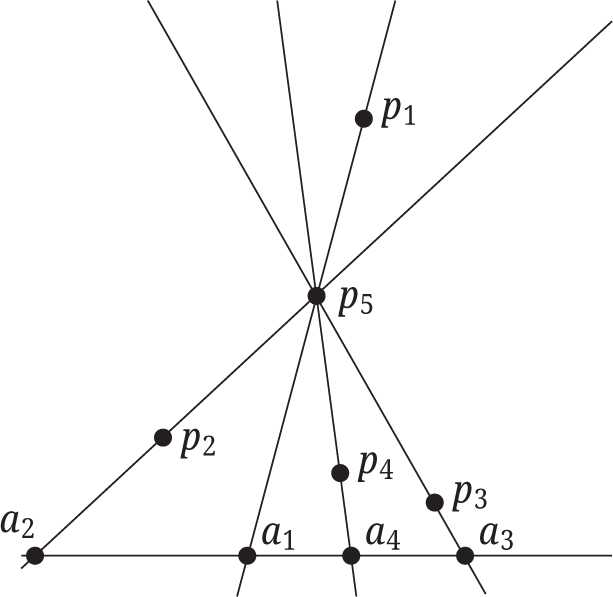
For distinct points p1, …, p5 ∈ ℙ2, the planar cross-ratio (p1, p2; p3, p4; p5) equals the 4 point cross-ratio (a1, a2; a3, a4).
Lemma 3.5
([29, Example 3.4.3]). A collection of 6 points p1, …, p6 ∈ ℙ2 lie on a conic if and only if
or generically, if the following cross-ratio equality holds:
Lemma 3.5 makes the following definition of a conic cross-ratio well-defined.
Definition 3.6
The conic cross-ratio of 4 points p1, …, p4 on a (non-degenerate) conic ω is
where p ∈ ω is any new point.
Any non-degenerate conic ω is isomorphic to ℙ1. If ι : ω → ℙ1 is one such isomorphism then
4 The cases k ≤ 4
We will now answer Problem 1.3 in the cases k ≤ 4. As a warm up to Problem 1.3 we first consider the analogous question in ℙ1 × ℙ1. Recall that any condition on a proper subset of {(xi, yi)} that makes the corresponding rows of Zk dependent is called an inherited condition for the rank drop of Zk.
Theorem 4.1
Consider the k × 4 matrix Zk =
rank(Z2) < 2 if and only if x1 = x2 and y1 = y2,
rank(Z3) < 3 if and only if either an inherited condition holds or x1 = x2 = x3 or y1 = y2 = y3,
rank(Z4) < 4 if and only if the following bracket equation holds:
Generically, x1, …, x4 and y1, …, y4 are distinct and then (16) holds if and only if there is a homography H ∈ PGL(2) such that Hxi = yi for i = 1, …, 4.
Proof
In each of the above cases, Zk will be rank deficient if and only if all its maximal minors vanish. Hence we compute the ideal of k × k minors of the symbolic Zk in each case and decompose it to understand rank deficiency. While computations in Macaulay2 are done over ℚ, our results hold over ℂ as explained at the end of the Introduction. By Corollary 2.2 we can fix the last coordinates of xi and yi to 1.
If k = 2 the ideal of 2 × 2 minors of Z2 is the prime ideal 〈x11 – x21, y11 – y21〉 which says that rank drops if and only if x1 = x2 and y1 = y2. We will call this the repeated point condition.
If k = 3, the ideal of 3 × 3 minors of the symbolic Z3 matrix is radical and decomposes into 5 prime ideals. Three of them correspond to repeated points xi = xj and yi = yj for i ≠ j. These are inherited for rank drop from the k = 2 case. The remaining 2 prime ideals say that x1 = x2 = x3 and y1 = y2 = y3 respectively.
When k = 4, we can use Macaulay2 to check that
which yields (16). In this case, the ideal of maximal minors is principal and prime, generated by det(Z4), and does not decompose. However, note that the bracket expression for det(Z4) vanishes under all of the conditions inherited from k = 2 and k = 3. Furthermore, when the xi’s and yi’s are distinct then (16) is equivalent to (x1, x2; x3, x4) = (y1, y2; y3, y4) and the homography follows by Lemma 3.3.□
We now consider Problem 1.3 for k ≤ 4 points (xi, yi) ∈ ℙ2 × ℙ2. Again all of the statements can be checked in Macaulay2 by following the same general strategy as in the proof of Theorem 4.1.
Theorem 4.2
Suppose that (xi, yi) ∈ ℙ2 × ℙ2 and Zk =
rank(Z2) < 2 if and only if x1 = x2 and y1 = y2.
rank(Z3) < 3 if and only if either an inherited condition holds or x1 = x2 = x3 and y1, y2, y3 are on a line, or x1, x2, x3 are on a line and y1 = y2 = y3.
rank(Z4) < 4 if and only if an inherited condition holds or one of the following is true:
x1 = x2 = x3 = x4 or y1 = y2 = y3 = y4.
The points x1, …, x4 ∈
Generically, the collinear points x1, …, x4 and y1, …, y4 are distinct and then (17) holds if and only if there is a homography H ∈ PGL(3) such that Hxi = yi for i = 1, …, 4.
Proof
The proof of (1) and (2) can be done using Macaulay2 by computing the ideal of maximal minors of Zk and then decomposing the radical of the ideal to get all possible conditions for rank drop. The matrix Zk is written symbolically as in (3) where by Corollary 2.2 we assume that the last coordinates of all xi’s and yi’s are 1. For instance, the ideal of 3 × 3 minors of Z3 is radical and of dimension 8 and degree 3. It is the intersection of 5 prime ideals of which 3 correspond to the repeated point conditions inherited from k = 2. The fourth ideal provides the new condition that x1 = x2 = x3 and y1, y2, y3 are on a line. The fifth ideal provides the analogous condition with the roles of x and y switched. These ideals appear in the form
The ideal of maximal minors of Z4 is radical of dimension 12 and degree 6. It decomposes into 17 primes ideals:
6 of the primes correspond to repeated points (inherited from k = 2). All of these have dimension 12 and degree 1.
8 of the primes correspond to 3 points on one side coinciding and the corresponding points on the other side on a line (inherited from k = 3). All of these ideals have dimension 11 and degree 2.
2 of the primes say x1 = x2 = x3 = x4 and y1 = y2 = y3 = y4 respectively (new conditions for k = 4). These ideals have dimension 10 and degree 1.
The last prime component, call it J, has dimension 11 and degree 24. It implies that the xi and yi are on a line (new condition for k = 4). One way to verify this claim is to check that the ideal generated by the brackets [123]x, [124]x and [123]y, [124]y is contained in J. These brackets being 0 encode the collinearity of xi’s and the collinearity of yi’s.
One can understand J more precisely by making the following calculation. If the x and y points are both on a line, then we can use homographies to fix these lines, and assume that xi = (ai, 0, 1) and yi = (bi, 0, 1) for i = 1, …, 4. This means that we can identify xi with (ai, 1) ∈ ℙ1 and yi with (bi, 1) ∈ ℙ1. Under this substitution, Z4 has exactly one non-zero minor
The second equality in (18) can be checked in Macaulay2. The bracket expression set to 0 is the equality of cross-ratios
which becomes well-defined when the xi’s are distinct and the yi’s are distinct.□
5 The case k = 5
We now consider the rank deficiency of Z5. In this case, we present two theorems. Theorem 5.1 is a characterization of rank deficiency in terms of brackets. We will see that a necessary condition for rank drop is that one set of points (say {yi}) is on a line ℓ. Theorem 5.2 gives a geometric characterization of rank deficiency when the points are sufficiently generic, i.e., when the yi’s on the line ℓ are distinct and the xi’s are in general position. In this case the rank drop of Z5 is equivalent to the existence of an isomorphism from the conic ω through the xi’s to the line ℓ taking xi to yi. This is analogous to Theorem 4.2 (3)(b) where there is a homography taking xi to yi under sufficient genericity. We will illustrate both results using Example 2.
Theorem 5.1
Given a configuration
By the action of permutations, there are only 5 equations to consider in (19), one for each choice of j ∈ {1, 2, 3, 4, 5}. If both the xi’s and the yi’s are contained in lines then (19) holds automatically. Generically, (19) is equivalent to the cross-ratio equalities
for all distinct i1, i2, i3, i4, j ∈ {1, 2, 3, 4, 5}.
Proof
The proof splits into two cases. For the first case, we assume that the points in neither side are entirely on a line and show that rank will drop only under inherited conditions. For the second case, we are then free to assume that one side is contained in a line, which allows us to simplify the Macaulay2 calculations.
Suppose that neither the xi’s nor the yi’s are on a line, and none of the inherited conditions hold. Then we can assume without loss of generality that x1 ≠ x2 and y1 ≠ y2 because no side has four coincident points (due to the absence of inherited conditions). Since neither side is contained entirely in a line, we can also assume that x1, x2, x3 are not collinear. Then either y1, y2, y3 are also not collinear, or y1, y2, y3 are on a line which means that we can assume that y1, y2, y4 are not collinear. Applying homographies, we therefore need to work with two different fixings of points:
and
Note that these fixings are not to finite points as we have done so far, but are equivalent to the fixing in (4) as remarked after Corollary 2.2. They allow for faster computations in Macaulay2.
In (21), the ideal generated by the 5 × 5 minors of Z5 is the intersection of 20 prime ideals. Of these, 4 correspond to invalid inputs xi, yi = (0, 0, 0); 7 correspond to the inherited repeated point condition from Theorem 4.2(1); 6 correspond to the inherited condition from Theorem 4.2(2); and the remaining 3 correspond to the inherited bracket/cross-ratio condition from Theorem 4.2(3)(b).
In (22), the ideal generated by the 5 × 5 minors of Z5 is the intersection of 17 prime ideals. Of these, 4 correspond to invalid inputs xi, yi = (0, 0, 0); 7 correspond to repeated points; 4 correspond to the inherited condition from Theorem 4.2(2); and the remaining 2 correspond to the inherited bracket/cross-ratio condition from Theorem 4.2(3)(b).
Thus, there are no new conditions for rank drop if neither the xi’s nor the yi’s are in a line.
Suppose that y1, …, y5 are on a line. Applying homographies, we may assume that yi = (mi, 0, 1) for i = 1, …, 5 and all xi are finite. We may further assume that x1 = (0, 0, 1) and that y1 = (0, 0, 1). Then rearranging the columns of Z5 we get
Let I be the ideal generated by the 6 non-zero 5 × 5 minors of
Example 2
The following example illustrates Theorem 5.1 and motivates Theorem 5.2. Consider
Here the yi’s are on the line yi = (mi, 0, 1) and we can verify that (19) is satisfied. The matrix
has rank 4.
Note that in this example, the yi’s (which are on a line) are distinct, and that no 3 of the xi’s are on a line. In this case, there is a 1-parameter family of rank 2 projective transformations {Tλ} such that Tλ (xi) = yi for i = 1, …, 5 except for 5 unique values of λ, one for each of x1, …, x5. In this example, this is the family
For each i = 1, …, 5 there exists unique λi such that Tλi has nullvector (center) xi. These are
Since Tλi (xi) = (0, 0, 0) ≁ yi, these 5 transformations can be seen as degenerate members of the family.
We now formalize the second half of Example 2 as a theorem. As seen in Theorem 5.1, for Z5 to drop rank, either the xi’s or the yi’s have to be on a line. Suppose the yi’s are distinct and on a line, and the xi’s are in general position. Then the xi’s lie on a conic ω and we will see that there is an isomorphism taking ω to the line containing the yi’s so that each xi maps to yi.
Theorem 5.2
Suppose that we have a configuration
The matrix Z5 is rank deficient.
For all c ∈ ω ∖ {x1, …, x5} there exists a projective transformation Tc : ℙ2 → ℙ1 centered at c such that Tc (xi) ∼ yi for all i.
For some c ∈ ω ∖ {x1, …, x5} there exists a projective transformation Tc : ℙ2 → ℙ1 centered at c such that Tc(xi) ∼ yi for all i.
There exists a cross-ratio preserving isomorphism F : ω → ℓy such that F(xi) = yi for all i.
Proof
To prove that (1) implies (2), let c ∈ ω ∖ {x1, …, x5}. Then for all distinct i1, i2, i3, i4, j ∈ {1, …, 5}
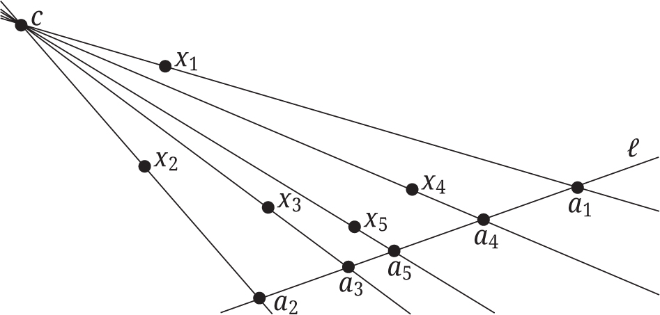
for any c ∈ ω. The first equation is from (20) in Theorem 5.1 and the other two equalities follow by Definition 3.6. Let cxi be the line through c and xi and let ℓ be any line such that c ∉ ℓ. Then if we define ai to be the unique intersection of ℓ and cxi it follows that
for all i1, i2, i3, i4 ∈ {1, …, 5}. See Figure 2. It follows that there exists homography H such that Hai ∼ yi for all i. Therefore if
We construct the projection with center c.
Clearly (2) implies (3). To show that (3) implies (1), suppose that such a projection exists and is centered at c. Then
for all distinct i1, i2, i3, i4, j ∈ {1, …, 5}. The first two equalities follow by Definition 3.6 and the last equality follows by hypothesis. It immediately follows that Z5 is rank deficient by Theorem 5.1.
To show that (1) implies (4) we may assume that the cross-ratio equalities (20) hold. Then define an isomorphism F : ω → ℓy by F(x1) = y1, F(x2) = y2, F(x3) = y3. Then for all p ∈ ω ∖ {x1, x2, x3}, F(p) = q is such that (x1, x2; x3, p)ω = (y1, y2; y3, q). It then follows that F(x4) = y4 and F(x5) = y5 because
by hypothesis (Theorem 5.1).
Finally, to show that (4) implies (1), suppose that such an isomorphism F exists. Then
for all i1, i2, i3, i4, j ∈ {1, …, 5}. The first equality follows by Definition 3.6 and the second and third equalities follow by hypothesis. It then follows that Z5 is rank deficient by Theorem 5.1.□
6 The case k = 6
The final case we will consider in this paper is a set of 6 inputs
We say that p1, …, p6 ∈ ℙ2 are in general position if at most 2 points are on a line and at most 5 points are on a conic. In several results below we need that the x points and/or the y points are in general position. We will also need that a collection of point pairs {(xi, yi)} ⊂ ℙ2 × ℙ2 is in general position, by which we mean that
the x points and y points are in general position, and
no more than 4 pairs (xi, yi) are related by a homography Hxi = yi.
Note that if (1) holds then Z5 has full rank because all of our previous conditions for rank drop require at least the xi’s or the yi’s to be on a line.
The variety ℙ2 × ℙ2 can be embedded in ℙ8 as the image of the Segre map
In what follows it will be helpful to identify ℙ8 with the set of all complex 3 × 3 matrices up to scaling via the bijection M ↔ vec(M). Then the Segre embedding of ℙ2 × ℙ2 in ℙ8 (which we also call ℙ2 × ℙ2) can be identified with the set of rank one 3 × 3 matrices up to scaling since
The Segre variety ℙ2 × ℙ2 ⊂ ℙ8 has dimension 4 and degree 6. It is the zero locus of the determinantal ideal generated by the 2 × 2 minors of a symbolic 3 × 3 matrix whose entries denote the coordinates of ℙ8.
We first show that given 5 points
Lemma 6.1
Let
then the 6th point has the formula
Proof
Let 𝓡(Z5) denote the row span of Z5 =
To prove the second part of the lemma, we first use homographies to fix the first 4 points as mentioned. We can then use Macaulay2 to verify that we can solve for (x6, y6) in terms of (x5, y5) as in equations (31).□
The existence of, and constructions for, this 6th point were noted in both [25] and [31], but not the rational formula. The rational formula shows that if
Example 3
We begin with 5 point pairs
If we leave (x6, y6) symbolic and construct the matrix Z6, we can verify with Macaulay2 that the unique new point pair that will result in rank deficiency is
In Lemma 6.16 we will prove a counterpart to the above result, where we instead begin with x1, …, x6 and calculate (up to homography) the points y1, …, y6 that will result in rank deficiency.
6.1 Algebraic characterizations of rank deficiency
In this subsection we will write down various algebraic characterizations of rank deficiency. While these statements are by no means obvious or intuitive, once stated, they are straightforward to check using Macaulay2. In the next section we explain the geometric origins of these statements.
Our first result is a characterization of rank drop using brackets and cross-ratios as in the previous sections.
Definition 6.2
Given 6 input points (xi, yi) ∈ ℙ2 × ℙ2, let 𝓑rackets(Z6) be the ideal generated by the differences of the two sides in the following bracket equations
for all distinct indices i, j, k, r, p, s ∈ {1, 2, 3, 4, 5, 6}.
Up to permutations, there are 30 equalities in (32): one for each choice of p and s. Under sufficient genericity, the bracket equations are the planar cross-ratio equalities
Next we define a specific kind of highly degenerate configuration.
Definition 6.3
We say that
Lemma 6.4
Let
Proof
We may assume up to reordering that y1 = y2 =: v1, y3 = y4 =: v2, y5 = y6 =: v3, x1 = x4 =: u1, x2 = x5 =: u2, and x3 = x6 =: u3. If u1, u2, u3 and v1, v2, v3 are both non-collinear, then we can assume by change of coordinates that u1 = v1 = (1, 0, 0), u2 = v2 = (0, 1, 0) and u3 = v3 = (0, 0, 1). It is then simple to check that Z6 has full rank.
If the three of points of one type are distinct but collinear and the three points of the other type are non-collinear, then we may assume up to change of coordinates and relabeling that u1 = v1 = (1, 0, 0), u2 = v2 = (0, 1, 0), u3 = (1, 1, 0), and v3 = (0, 0, 1). Again, it is simple to check that Z6 has full rank.
If two points of one type are coincident, say u1 = u2, then an inherited condition holds and the rank drops. If u1, u2, u3 and v1, v2, v3 are both collinear then again the rank drops due to an inherited condition.□
Let 𝓜inors(Z6) denote the ideal of maximal minors of Z6. The following statement can be checked using Macaulay2.
Theorem 6.5
Let
Proof
As in the proof of Theorem 5.1 we split into two cases. Applying homographies we can assume that
or
In the first case the ideal 𝓜inors(Z6) decomposes into 19 components. The first 6 correspond to invalid inputs xi, yi = (0, 0, 0), the next 12 correspond to repeated point pairs, and the 19th component we refer to as M19. The ideal 𝓑rackets(Z6) decomposes into 13 components. One component is M19 and the other 12 components correspond to asymmetric double triangles.
In the second case the ideal 𝓜inors(Z6) decomposes into 17 components. The first 6 correspond to invalid inputs xi, yi = (0, 0, 0), the next 10 correspond to repeated point pairs, and the 17th component we refer to as M17. The ideal 𝓑rackets(Z6) decomposes into 21 components. One component is M17 and the other 20 components correspond to asymmetric double triangles.□
In Theorem 6.5 the only assumption is that neither the xi’s nor the yi’s are on a line. In Theorem 6.8 we will tackle the case of one side in a line, and together the two theorems cover all possibilities.
Before we can do that, we consider an important subcase of Theorem 6.5, namely the generic case. The main result here is Theorem 6.7 which uses tools from invariant theory that we have not encountered thus far. Besides being a key result of this paper, it will also lead to a proof of Theorem 6.8, completing the story.
Suppose that x1, …, x6 ∈
and consider the rank deficiency of Z6 whose 5th and 6th rows are left symbolic as
Recall that the general position assumption guarantees that no submatrix of Z6 with 5 rows is rank deficient. Under these assumptions, one can use Macaulay2 to check that 𝓜inors(Z6) is a radical ideal of dimension 9 and degree 4. Its prime decomposition consists of 14 components. The first 4 of these components correspond to invalid inputs xi, yi = (0, 0, 0), the next 9 correspond to repeated points, and the 14th component, denoted as M14, encodes a new set of conditions, and has dimension 8 and degree 35. Since Z6 is rank deficient if and only if all its maximal minors vanish, we conclude that the new conditions for rank drop are exactly that (x5, y5) and (x6, y6) lie in the variety of M14.
We will now interpret M14 in terms of the invariants of x1, …, x6 and y1, …, y6. For a set of 6 points p1, …, p6 ∈ ℙ2 define
This is a classical invariant of points in ℙ2 whose vanishing expresses that the three lines pipj, pkpl and prps meet in a point; see [6, page 169]. Using these invariants, Coble defines the following 6 scalars in [6, page 170]:
Let āx, b̄x, c̄x, d̄x, ēx, f̄x be the polynomials obtained by computing the expressions in (37) using 6 symbolic vectors x1, …, x6 where each xi = (xi1, xi2, xi3)⊤. Similarly, let āy, b̄y, c̄y, d̄y, ēy, f̄y be obtained from symbolic vectors y1, …, y6 where each yi = (yi1, yi2, yi3)⊤.
Definition 6.6
Let 𝓘nvariants(Z6) denote the ideal of 2 × 2 minors of
after specializing the first 4 points (xi, yi) as in (34).
The ideal 𝓘nvariants(Z6) is radical of dimension 9 and degree 4. Its prime decomposition consists of 14 components. The first 4 of these components correspond to invalid inputs xi, yi = (0, 0, 0), the next 8 correspond to 3 repeated points in either
Theorem 6.7
Given a configuration
if and only if either the matrix Z6 is rank deficient or yi = Hxi for some homography H ∈ PGL(3).
Proof
It can be checked using Macaulay2 that M14 = I14.□
The statement of Theorem 6.7 begs the question of how homography ties in with rank drop, if at all. We give an example to show that the existence of a homography such that yi = Hxi for 6 points (xi, yi) is not sufficient for Z6 to be rank deficient. In contrast, it does suffice for 7 point pairs.
Example 4
By Lemma 2.1, if there exists H ∈ PGL(3) such that yi = Hxi for i = 1, …, 6, then we may assume that xi = yi for i = 1, …, 6. Then the null space of Z6 consists exactly of the vectors vec(F) for the 3 × 3 matrices F such that
Generically, this is exactly the set of 3 × 3 skew-symmetric matrices, Skew3 ≅ ℙ2. Hence rank(Z6) = 6. For example, consider
for which the nullspace of Z6 is Skew3. In general, if the homography is given by the matrix H then the null space of Z6 is obtained by left action of H⊤ on Skew3. We note that this null space is unusual in that will always consist entirely of rank 2 matrices.
To finish our algebraic discussion, we consider the case of one ℙ2 having all input points in a line. In order to state the result, we introduce the classical Joubert invariants of 6 points in ℙ1, compare [6], which are
Theorem 6.8
Suppose that y1, …, y6 ∈
Furthermore, if x1, …, x6 are in general position and y1, …, y6 are distinct, then (42) holds if and only if there exists a projection T :
This theorem is analogous to Theorems 4.2 (3)(b) and 5.2. The proof of this theorem will follow from the geometry that we develop in the next subsection.
6.2 Geometric characterizations of rank deficiency
We next explain where the algebraic results (and ideals) from the previous section come from by providing a geometric characterization of rank deficiency of Z6. This relies on the classical theory of smooth cubic surfaces in ℙ3. For the convenience of the reader, we have collected the needed facts about cubic surfaces in Appendix A.
6.2.1 Cubic surfaces and Schäfli double sixes
A cubic surface in ℙ3 is a hypersurface defined by a single homogenous polynomial of degree 3 in ℂ[z0, z1, z2, z3] where (z0, …, z3) are the coordinates of ℙ3.
Definition 6.9
A pair of 6 lines {ℓ1, …, ℓ6} and
the 6 lines in each set are mutually skew (i.e., no 2 of them intersect), and
ℓi intersects
A smooth cubic surface has 36 Schläfli double sixes. The rich and highly symmetric properties of these line configurations are listed in Appendix A and lie at the heart of all of our major results in this section. Our main (geometric) theorem in this section is the following.
Theorem 6.10
Suppose that
When Z6 is rank deficient, this cubic surface has the determinantal representation 𝓝(Z6) ∩ 𝓓, where 𝓝(Z6) denotes the right null space of Z6 and 𝓓 is the cubic hypersurface of all rank deficient 3 × 3 matrices.
To prepare for the proof of this theorem, we begin by constructing a cubic surface from 5 points
is a cubic surface in 𝓝(Z5) ≅ ℙ3 ⊂ ℙ8. This surface is smooth by the general position assumption. (We note that if {xi} and {yi} were related by a homography then S would be degenerate; see Example 4.)
The surface S has a natural determinantal representation (see Appendix A for the definition): Pick a basis M0, …, M3 of 𝓝(Z5) and set
where zi ∈ ℂ. If (xi, yi) with i = 1, …, 5 are real, we can choose M0, …, M3 to be real matrices. Since M(z) is a parameterization of 𝓝(Z5), S is cut out by det(M(z)) = 0, and M(z) is a determinantal representation of S. Generically, the 3-dimensional 𝓝(Z5) does not intersect the 4-dimensional ℙ2 × ℙ2 of rank one matrices, and so a point M(z) on S has rank exactly 2. This also follows from S being smooth.
Next we construct a Schläfli double six on the cubic surface S = 𝓝(Z5) ∩ 𝓓 from
Definition 6.11
Given
where M(z) is of the form (44).
For each i = 1, …, 5 we have ℓxi ⊂ 𝓝(Z5) by the definition of M(z) in (44). Further, since M(z) xi = 0, M(z) has a non-trivial right null space and hence det(M(z)) = 0. Therefore ℓxi ⊂ S = 𝓝(Z5) ∩ 𝓓. The condition that M(z) ∈ 𝓝(Z5) is equivalent to M(z) satisfying the 5 linear constraints
Therefore, ℓxi is cut out by 8 linear constraints including the 3 constraints given by M(z) xi = 0. However one of them is redundant since M(z) xi = 0 implies that
Lemma 6.12
The lines ℓxi and
The lines {ℓxi, i = 1, …, 5} are mutually skew.
The lines {
ℓxi intersects
Therefore, {ℓxi, i = 1, …, 5} and {
Proof
The proof of the incidence relations follows from dimension counting and can be found in [25, Lemma 6.1]. The two sets of lines are part of a unique Schläfli double six on S since each double six is uniquely defined by three of its line pairs, and we have 5 line pairs here with the correct incidences; see Lemma A.1 (3).□
By Lemma A.1, given a Schläfli double six on S, there are two sets of 6 points {pi} ⊂
We are now ready to prove the forward direction of Theorem 6.10.
Definition 6.13
Let ℓ6,
Lemma 6.14
Suppose that
Proof
To prove the forward direction, suppose Z6 is rank deficient. Then 𝓝(Z5) = 𝓝(Z6) and S = 𝓝(Z6) ∩ 𝓓. Check that ℓx6 is a line on S by the same argument as for ℓxi with i ≤ 5. Similarly,
To prove the reverse direction, suppose we have a Schläfli double six on S as in the statement of the lemma. Then by the discussion before Definition 6.13, S is the blow up of
The following corollary to Lemma 6.14 and Theorem A.5 concludes the proof of the forward direction of Theorem 6.10.
Corollary 6.15
If
Note that Lemma 6.14 gives a second construction for the unique point pair (x6, y6) in Lemma 6.1, namely as the images under the blow up morphisms of the final pair of lines in the unique Schläfli double six on S determined by the lines
To prove the backward direction of Theorem 6.10, we will first prove a counterpart to Lemma 6.1.
Lemma 6.16
If x1, …, x6 are in general position, then there is a unique set of 6 points y1, …, y6 in general position (up to homography) such that Z6 is rank deficient. If we assume that
then we can obtain y5, y6 via the rational function
Proof
We first prove that this construction will result in rank deficiency; the uniqueness will come afterwards as a consequence of Corollary 6.15. We construct the matrix
To see that this choice is unique, construct S = 𝓝(Z6) ∩ 𝓓. Then by Corollary 6.15, S is both the blow up of
The formula shows that if x1, …, x6 are real then, up to homography, y1, …, y6 will also be real.
Example 5
Consider Example 3 again and now fix the points
If we leave y5, y6 symbolic and construct the matrix Z6, we can verify with Macaulay2 that the unique new points that will result in rank deficiency are y5 ∼ (8, 2, 1),
The following corollary now completes the reverse direction of Theorem 6.10.
Corollary 6.17
Given a smooth cubic surface 𝓢 with a Schläfli double six
Proof
Lemma 6.16 provides %%us with unique (up to homography) points
Combining Corollaries 6.15 and 6.17 we obtain a method to compute a determinantal representation of a smooth cubic surface starting with a Schläfli double six on it.
Corollary 6.18
Let 𝓢 be a smooth cubic surface with a Schläfli double six {ℓi} and
This gives us the final statement of Theorem 6.10, concluding the proof.
Remark 6.19
In the classical literature one finds a determinantal representation of a cubic surface from 6 points in a ℙ2 (whose blow up at these points is the surface), via the Hilbert–Burch theorem (see Appendix A). It is worthwhile to contrast that method with that in Corollary 6.18 where the starting point are 6 point pairs in ℙ2 × ℙ2. Then a determinantal representation (44) of the surface can be obtained from a basis of 𝓝(Z6) using simple linear algebra.
6.2.2 Conic intersections and the bracket ideal 𝓑rackets(Z6)
We now use Theorem 6.10 to explain the ideal 𝓑rackets(Z6) used in the algebraic characterization of rank deficiency in Theorem 6.5.
Consider a Schläfli double six
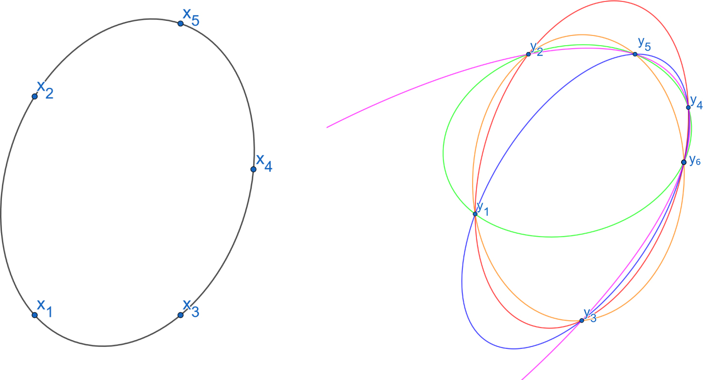
The point y6 is the unique intersection point of the 5 conics
Lemma 6.20
(See [28] and [31]). Let C be the unique conic through x1, …, x5 in general position, and let Hi be the unique homography such that yj = Hixj for all j ≠ i. Define
Similarly, let C′ be the unique conic through y1, …, y5 and let Gj be the unique homography such that xi = Gjyi for all i ≠ j. Define Cj := Hj(C′) for j = 1, …, 5. Then
We can now restate Theorem 6.10 using Lemma 6.20 to yield another characterization of minimal rank deficiency of Z6.
Theorem 6.21
Let
Theorem 6.21 explains the bracket and cross-ratio conditions that appear in Theorem 6.5. Let C be the conic through x1, …, x5 and let H be the homography such that Hxi = yi for i = 1, 2, 3, 4. Then C′ := HC is a conic that passes through y1 = Hx1, y2 = Hx2, y3 = Hx3, y4 = Hx4 and Hx5. By Lemma 3.5, y6 ∈ C′ if and only if
This can be rewritten as the bracket equation (32) by eliminating det(H):
The other 29 bracket equations follow by selecting different conics and homographies.
6.2.3 The Cremona hexahedral form of a cubic surface
We now give a third characterization of minimal rank deficiency of Z6 via the Cremona hexahedral form of a cubic surface. This will explain the statement of Theorem 6.7.
Recall that every smooth cubic surface is the blow up of ℙ2 at 6 points in general position. The Cremona hexahedral form of the surface provides explicit equations for it in terms of the points being blown up. We briefly describe these equations and the properties we need. More details can be found in [6, Section 4], [13, Section 9.4.3] and [24, Section 5.6].
Given 6 points p1, …, p6 ∈ ℙ2, consider the following list of 6 cubic polynomials in u = (u0, u1, u2), the coordinates of ℙ2, that vanish on them:
In fact, each summand in each cubic is the product of the lines through 3 disjoint pairs of the 6 points and already vanishes on the points. Formally these expressions are similar to the scalars in (37). These cubic polynomials are covariants of p1, …, p6 under the action of PGL(3), and appear in the work of Coble [6].
The 6 cubics in (53) span the 4-dimensional vector space of cubics that vanish on p1, …, p6 and can be used to blow up ℙ2 at p1, …, p6 to obtain a cubic surface S. This surface is the closure of
and the zero set of the Cremona hexahedral equations
where the scalars ā, …, f̄ are as in (37). Here, z1, …, z6 are the coordinates of ℙ5.
The Cremona hexahedral form of S can be used to find the 27 lines on S explicitly via expressions for the 45 tritangent planes of S, see [6, Section 4]. In particular the 15 lines that are not part of the Schläfli double six corresponding to the blow up are obtained by permuting the equations
Under the blow up morphism π : S → ℙ2, these lines correspond to specific lines pipj; the one above corresponds to the line between p1 and p2.
We can characterize the rank deficiency of Z6 via the Cremona hexahedral form.
Theorem 6.22
Let x1, …, x6 ∈
Proof
If Sx = Sy, then they both contain the 15 lines in equation (56), none of which correspond to the proper transforms of either set of 6 points under their respective blow up morphisms. It follows that either the exceptional lines of x1, …, x6 are exactly the exceptional lines of y1, …, y6 or that the two sets are entirely distinct. Moreover, since each of the 15 lines in (56) have specific intersection conditions, either ℓxi = ℓyi for all i, or {ℓx1, …, ℓx6} and {ℓy1, …, ℓy6} form a Schläfli double six.
In the first case, the exceptional lines of x1, …, x6 are exactly the exceptional lines of y1, …, y6. Then we can define an invertible projective transformation πy ∘
In the second case the exceptional lines of x1, …, x6 are distinct from the exceptional lines of y1, …, y6. In this case they form a Schläfli double six and by Theorem 6.10, Z6 is rank deficient.
To prove the reverse direction, suppose that Hxi = yi for some homography H. Then Sx = Sy because (āx, … f̄x) ∼ (āy, …, f̄y) by the formula in (37) which means that Sx and Sy have the same Cremona hexahedral form. Similarly, if Z6 is rank deficient then by Theorem 6.10,
Theorem 6.22 provides a geometric proof of the algebraic characterization of rank deficiency in Theorem 6.7. As before, we index %subscript the cubics in (53) with x or y depending on whether they come from {xi} or {yi}. The Cremona hexahedral equations (55) imply that the two cubic surfaces Sx and Sy are equal if and only if the following polynomials in u (coordinates on
In other words,
or equivalently, the matrix
is rank deficient. One can check using Macaulay2 that the ideal of 3 × 3 minors of (59) coincides with the ideal 𝓘nvariants(Z6) of 2 × 2 minors of (38). Therefore, we conclude that Sx and Sy coincide if and only if (39) holds, which is the same as
for some non-zero scalar λ.
This concludes the discussion about 6 points
6.2.4 The Proof of Theorem 6.8
We can now use the tools developed in the previous subsection to prove Theorem 6.8 which is the last statement left to prove. This is the case of one ℙ2 having all input points on a line; suppose this is
and for all points v ∈
where Ay, …, Fy are the Joubert invariants introduced in (41). The Joubert invariants are known to satisfy
see [13, Theorem 9.4.10], and any 5 of them give a complete basis for the space of invariants for 6 ordered points in ℙ1. In particular, if p1, …, p6 ∈ ℙ1 and q1, …, q6 ∈ ℙ1 are two sets of 6 distinct points, then there exists a homography H sending pi ↦ qi if and only if
We further note that if
The following lemma proves the first part of Theorem 6.8.
Lemma 6.23
Let
Proof
The proof is relatively straightforward. Suppose that y1, …, y6 are on a line. Applying homographies to each side we may assume that the xi’s are all finite and that yi = (yi1, 1, 0). Then
and Z6 is rank deficient if and only if its only obviously non-zero 6 × 6 minor det(M) = 0. Furthermore, a quick computation will give
yielding the desired result.□
Before we prove the second part of Theorem 6.8, we compute an example to illustrate the statement.
Example 6
Consider the following points in which the x points are in general position and the y points are all distinct and contained in a line. This can be seen as a configuration in ℙ2 × ℙ1 so we fix
and leave x6, y6 as symbolic finite points. This creates a 6 × 6 matrix
(The reader may also view the yi as points on the line at infinity in ℙ2 where the third coordinate is 0; the non-zero part of the corresponding 6 × 9 matrix Z6 is (66).)
The matrix Z6 in (66) is rank deficient exactly when its determinant, a quadratic polynomial in the coordinates of x6 and y6, is 0. If we arbitrarily fix x6 = (2, 11, 1), then det(Z6) = –918y61 + 2942, and y6 = (2942, 918) is the unique point y6 such that the configuration is rank deficient.
If we consider only the first 5 point pairs we fixed initially, there exists a unique projective transformation
such that Txi ∼ yi for all i = 1, …, 5. Moreover, we can check that Tx6 = (–2942, –918) ∼ y6. This transformation T has center u = (–1617, –803, 11888). This point actually has some further significance, because we can check that (ax(u), …, fx(u)) ∼ (48079, –55599, –88559, –17265, 22529, 90815) ∼ (Ay, …, Fy).
The following now finishes the proof of Theorem 6.8.
Proof of Theorem 6.8
(second part). Let S be the blow up of
We first show that if Z6 is rank deficient then a projection exists. Let ℓ ⊂
Since the Joubert invariants generate the space of all invariants for 6 ordered points on a line, it follows that there exists a homography H : ℓ →
To prove the reverse direction, suppose that such a projection T exists. We can use homography on each side to fix u = (0, 0, 1) and to fix the image line at infinity. Equivalently, pick homographies on each side such that
It then follows that xi = (yi1, yi2, bi) for all i, where the bi are unknown scalars. The matrix Z6 then becomes
which is clearly rank deficient. This concludes the proof of Theorem 6.8.□
Funding statement: A.E. is supported by NSF CCF 2110075.
Acknowledgements
We thank Jarod Alper, Timothy Duff, and Giorgio Ottaviani for helpful discussions.
Communicated by: D. Plaumann
References
[1] M. Bertolini, L. Magri, C. Turrini, Critical loci for two views reconstruction as quadratic transformations between images. J. Math. Imaging Vision 61 (2019), 1322–1328. MR4017694 Zbl 1482.68246Search in Google Scholar
[2] M. Bråtelund, Critical configurations for three projective views. Math. Scand. 129 (2023), 401–444. MR4667876 Zbl 07849503Search in Google Scholar
[3] M. Bråtelund, Critical configurations for two projective views, a new approach. J. Symbolic Comput. 120 (2024), Paper No. 102226, 22 pages. MR4583113 Zbl 07725351Search in Google Scholar
[4] A. Buckley, T. Košir, Determinantal representations of smooth cubic surfaces. Geom. Dedicata 125 (2007), 115–140. MR2322544 Zbl 1117.14038Search in Google Scholar
[5] P. Bürgisser, F. Cucker, Condition. The geometry of numerical algorithms, volume 349 of Grundlehren Math. Wiss. Springer 2013. MR3098452 Zbl 1280.65041Search in Google Scholar
[6] A. B. Coble, Point sets and allied Cremona groups. I. Trans. Amer. Math. Soc. 16 (1915), 155–198. MR1501008 Zbl 02618070Search in Google Scholar
[7] E. Connelly, R. Thomas, C. Vinzant, The geometry of rank drop in a class of face-splitting matrix products: Part II. Adv. Geom. 24 (2024), 395–420.Search in Google Scholar
[8] J. W. Demmel, The geometry of ill-conditioning. J. Complexity 3 (1987), 201–229. MR907197 Zbl 0641.65042Search in Google Scholar
[9] J. W. Demmel, On condition numbers and the distance to the nearest ill-posed problem. Numer. Math. 51 (1987), 251–289. MR895087 Zbl 0597.65036Search in Google Scholar
[10] J. W. Demmel, Applied numerical linear algebra. Society for Industrial and Applied Mathematics (SIAM), Philadelphia, PA 1997. MR1463942 Zbl 0879.65017Search in Google Scholar
[11] H. Derksen, G. Kemper, Computational invariant theory, volume 130 of Encyclopaedia of Mathematical Sciences. Springer 2015. MR3445218 Zbl 1332.13001Search in Google Scholar
[12] I. Dolgachev, D. Ortland, Point sets in projective spaces and theta functions. Astérisque no. 165 (1988), 210 pages (1989). MR1007155 Zbl 0685.14029Search in Google Scholar
[13] I. V. Dolgachev, Classical algebraic geometry. Cambridge Univ. Press 2012. MR2964027 Zbl 1252.14001Search in Google Scholar
[14] D. Eisenbud, Commutative algebra. Springer 1995. MR1322960 Zbl 0819.13001Search in Google Scholar
[15] H. Fan, J. Kileel, B. Kimia, On the instability of relative pose estimation and RANSAC’s role. In: Proc. IEEE/CVF Conference on Computer Vision and Pattern Recognition, 2022, 8925–8933.Search in Google Scholar
[16] D. R. Grayson, M. E. Stillman, Macaulay2, a software system for research in algebraic geometry. www.math.uiuc.edu/Macaulay2/.Search in Google Scholar
[17] R. Hartley, F. Kahl, Critical configurations for projective reconstruction from multiple views. International Journal of Computer Vision 71 (2007), 5–47. Zbl 1477.68366Search in Google Scholar
[18] R. Hartley, A. Zisserman, Multiple view geometry in computer vision. Cambridge Univ. Press 2003. MR2059248 Zbl 1072.68104Search in Google Scholar
[19] R. Hartshorne, Algebraic geometry. Springer 1977. MR463157 Zbl 0367.14001Search in Google Scholar
[20] D. Hilbert, S. Cohn-Vossen, Geometry and the imagination. Chelsea Publishing Co., New York 1952. MR46650 Zbl 0047.38806Search in Google Scholar
[21] F. Kahl, R. Hartley, Critical curves and surfaces for euclidean reconstruction. In: Computer Vision 2002: 7th European Conference on Computer Vision, Copenhagen 2002, Proc. Part II, Lect. Notes Comput. Sci. 2351, Springer 2002, 447–462. Zbl 1039.68658Search in Google Scholar
[22] C. G. Khatri, C. R. Rao, Solutions to some functional equations and their applications to characterization of probability distributions. Sankhyā Ser. A 30 (1968), 167–180. MR238416 Zbl 0176.49004Search in Google Scholar
[23] Q. T. Luong, O. D. Faugeras, The fundamental matrix: Theory, algorithms, and stability analysis. International Journal of Computer Vision 17 (1996), 43–75.Search in Google Scholar
[24] G. Ottaviani, Five lectures on projective invariants. Rend. Semin. Mat. Univ. Politec. Torino 71 (2013), 119–194. MR3345059 Zbl 1312.13012Search in Google Scholar
[25] A. Pryhuber, R. Sinn, R. R. Thomas, Existence of two view chiral reconstructions. SIAM J. Appl. Algebra Geom. 6 (2022), 41–76. MR4387191Search in Google Scholar
[26] J. G. Semple, G. T. Kneebone, Algebraic projective geometry. Oxford Univ. Press 1998. MR1651410 Zbl 0932.51008Search in Google Scholar
[27] V. I. Slyusar, A family of face products of matrices and its properties (Russian). Kibernet. Sistem. Anal. no. 3 (1999), 43–49, 189. English translation in Cybernet. Systems Anal. 35 (1999), no. 3, 379–384. MR1728929 Zbl 0984.15015Search in Google Scholar
[28] R. Sturm, Die Lehre von den geometrischen Verwandtschaften. Dritter Band: Die eindeutigen linearen Verwandtschaften zwischen Gebilden dritter Stufe. Teubner, Leipzig 1909. Zbl 39.0604.01Search in Google Scholar
[29] B. Sturmfels, Algorithms in invariant theory. Springer 2008. MR2667486 Zbl 1154.13003Search in Google Scholar
[30] C. F. Van Loan, The ubiquitous Kronecker product. J. Comput. Appl. Math. 123 (2000), 85–100. MR1798520 Zbl 0966.65039Search in Google Scholar
[31] T. Werner, Constraint on five points in two images. In: Proc. IEEE Conference on Computer Vision and Pattern Recognition 2 (2003), 203–208.Search in Google Scholar
A Appendix: Facts about cubic surfaces
This is a collection of classical facts about cubic surfaces needed in Subsection 6.2. See [19, V. Chapter 4] for a modern reference and [6] or [20] for classical references.
Lemma A.1
Let 𝓢 ⊂ ℙ3 be a smooth cubic surface. Then the following hold.
𝓢 can be obtained by blowing up 6 points p1, …, p6 ∈ ℙ2 in general position. The exceptional curves of p1, …, p6 in the blow up morphism π : 𝓢 → ℙ2 are 6 lines ℓ1, …, ℓ6 on 𝓢.
The cubic surface 𝓢 has exactly 27 (complex) lines. They are
the exceptional lines ℓ1, …, ℓ6,
the strict transforms ℓij of the lines in ℙ2 passing through pi, pj for 1 ≤ i < j ≤ 6 (15 of them), and
the strict transforms
The two sets of lines {ℓ1, …, ℓ6} and
Any set of 6 mutually skew lines among the 27 lines on 𝓢 can play the role of ℓ1, …, ℓ6. Precisely, if {g1, …, g6} is a set of 6 mutually skew lines among the 27 lines, then there is another morphism π′ : 𝓢 → ℙ2, making 𝓢 isomorphic to ℙ2 with six points q1, …, q6 in general position blown up such that g1, …, g6 are the exceptional curves of q1, …, q6 under π′.
We now note several facts about double sixes in ℙ3 (or more generally line configurations in ℙ3).
Lemma A.2
Each double six in ℙ3 is contained in a unique non-singular cubic surface and thus forms part of the set of 27 lines on that surface.
Any set of 6 mutually skew lines among 27 lines that satisfy the incidence relations is one half of a unique Schläfli double six and determines the other lines and the cubic surface.
Next we talk about determinantal representations of a cubic surface.
Definition A.3
A determinantal representation of a cubic surface 𝓢 defined by a cubic equation F(z) = F(z0, z1, z2, z3) = 0 is a 3 × 3 matrix of linear forms
such that det(M(z)) = λF(z) for some λ ≠ 0. Two representations M(z) and M′(z) are equivalent if M′(z) = AM(z)B with A, B ∈ GL(3).
Note that if M(z) is a determinantal representation of 𝓢, then so is M(z)⊤. We present the following facts about determinantal representations of a cubic surface; see [4].
Lemma A.4
Every smooth cubic surface 𝓢 has a determinantal representation.
The equivalence classes of determinantal representations of 𝓢 are in bijection with sets of 6 mutually skew lines on 𝓢 that are the exceptional curves of the blow up of ℙ2 at the 6 points that give 𝓢.
If the determinantal representation M of 𝓢 corresponds to the skew lines ℓ1, …, ℓ6 on 𝓢, then M⊤ corresponds to another 6 skew lines
The choice of a Schläfli double six ℓ1, …, ℓ6,
Here are various recipes to explicitly realize some of the above assertions.
If 𝓢 is the blow up of ℙ2 at the 6 points p1, …, p6, then 𝓢 can be constructed as follows. Pick a basis {f0, f1, f2, f3} of the 4-dimensional vector space of cubics through p1, …, p6 and map
The variety of 〈f0, …, f3〉 is {p0, …, p6}. By the Hilbert–Burch theorem [14, Section 20.4] there is a 3 × 4 matrix L(u) of linear forms in u0, u1, u2 whose maximal minors are f0, …, f3. The matrix L(u) generically has rank 3 and has rank 2 exactly when u = pi for some i = 1, …, 6. Define a 3 × 3 matrix M(z) of linear forms in z0, z1, z2, z3 by the relation
Then M(z) is a determinantal representation of 𝓢.
The blow up of ℙ2 at p1, …, p6 can be seen via (74). If ū ∈ ℙ2 is not one of p1, …, p6, then some fi(ū) ≠ 0 and rank(L(ū)) = 3. Therefore, the null space of L(ū) is a unique point z̄ ∈ ℙ3 and M(z̄)ū = L(ū)z̄ = 0. This means that det(M(z̄)) = 0 and z̄ ∈ 𝓢. If z̄ is a generic point on 𝓢, then rank(M(z̄)) = 2, and the blow up morphism π sends z̄ to the unique point ū ∈ ℙ2 that generates the right null space of M(z̄).
The 6 exceptional curves of the blow up are precisely
By what is stated above, rank(L(u)) = 2 if and only if u = pi for some i = 1, …, 6 if and only if (via (74)) M(z)u = L(u)z = 0 is a system of 2 linearly independent equations in z (i.e., defines a line in ℙ3). This line is entirely on 𝓢 since det(M(z)) = 0 if M(z)pi = 0.
Corresponding results hold for the determinantal representation M(z)⊤ of 𝓢.
To obtain the points q1, …, q6 ∈ ℙ2 whose blow up is 𝓢, compute L′(u) via
The variety of the maximal minors of L′(u) is {q1, …, q6}.
A point ȳ ∈ ℙ2 not equal to any qi is sent to the unique point z̄ in ℙ3 in the right nullspace of L′(ȳ). This means L′(ȳ)z̄ = M(z̄)⊤ ȳ = 0 and z̄ ∈ 𝓢 since det(M(z̄))⊤ = 0.
The morphism π′ : 𝓢 → ℙ2 sends z̄ to the unique point ȳ ∈ ℙ2 that generates the right nullspace of M(z̄)⊤, or equivalently, the left nullspace of M(z̄).
The exceptional curves of the blow up are the lines
The following theorem follows from the above facts.
Theorem A.5
Given a determinantal representation M(z) of a smooth cubic surface 𝓢 ⊂ ℙ3, there exists 6 points (pi, qi) ∈ ℙ2 × ℙ2 such that 𝓢 is the blow up of the first ℙ2 at
© 2024 Walter de Gruyter GmbH, Berlin/Boston, Germany
This work is licensed under the Creative Commons Attribution 4.0 International License.
Articles in the same Issue
- Frontmatter
- Automorphisms and opposition in spherical buildings of classical type
- Revisiting gradient conformal solitons
- Abelian branched covers of rational surfaces, II
- Annulus configurations in handlebody-knot exteriors
- Cones between the cones of positive semidefinite forms and sums of squares
- The geometry of rank drop in a class of face-splitting matrix products: Part I
- The geometry of rank drop in a class of face-splitting matrix products: Part II
- Triality and automorphisms of principal bundles moduli spaces