
The Differential Algorithm for American Put Option with Transaction Costs under CEV Model
-
Zhao Yin
 und
Chang Tan
und
Chang Tan

Abstract
This paper mainly studies the American put option pricing with transaction costs in the CEV process. The specific Crank-Nicolson form of numerical solution is obtained by the finite difference method. On this basis, Hong Kong stock CKH option is selected as the object to estimate option price. Finally, by comparing with the actual price, the American put option pricing model is verified as reasonable. This paper is significant to the rational pricing and the institutional construction of the upcoming stock options in mainland China.
1 Introduction
Since the 1980’s, marginal utility and certainty equivalence principle were applied to the field of financial derivatives pricing. Based on this theory, the method of option pricing and hedging was proposed by Hodges and Neuberger[1]. Davis et al developed the pricing model by Hodges and Neuberger under the hypothesis of a proportional transaction costs in the market[2]. Then, Clewlow and Hodges[3], Damgaard[4–5] and Monoyios[6] further studied the option pricing method based on utility theory. All these studies above assumed that the stock price volatility process follows Geometric Brownian Motion. It is important to note that the empirical test on stock prices and stock index did not verify the logarithmic normal assumption. Therefore, stochastic process gained widely attention and was applied to the option pricing theory as the alternative method. For example, Cox and Rubinstein made a research on the CEV (Constant Elasticity of Variance) process[7].
There are many domestic scholars focus on the CEV process in recent 10 years. Wu and He established binary tree pricing model as the stock price follows geometric Asian option of CEV process[8]. Du and Ding established the binary option pricing model as stock price follows the CEV process, and the numerical solution is given by finite difference method[9]. Qin and Zheng also use finite difference method to study European call option with transaction cost as stock prices follow the CEV process, and numerical solution method is given[10]. Yuan and Shi studied the utility indifference pricing with proportional transaction costs under the CEV process and its numerical solution[11]. This paper studied the differential equation model of option pricing with transaction costs under CEV process, and modified the boundary condition of model by using finite difference method to get the numerical solution of American put options. The innovation is that we obtained the numerical solution of American option pricing with transaction costs under CEV process.
2 The research on option pricing with transaction costs under CEV process
2.1 Introduction to the CEV model
Constant Elasticity of Variance model, which referred to as CEV model, means that elasticity of variance is constant. It is a natural extension of Geometric Brownian Motion[12].
Let σ(S(t)) be variance of stock price S(t), we may have
Under CEV process the volatility of stock price takes the form
where 0 ⩽ α ⩽ 1, µ is the drift rate, σ2 is the variance of stock price volatility and B(t) deotes Brownian Motion.
When α = 1, volatility of stock price satisfies dS(t) = µSdt + σSdB(t), the Geometric Brownian Motion. When α = 1/2 and α = 0, it satisfies
The differential equation of the price of put option with transaction costs under the CEV process takes the form
Equation (1) is a second-order nonlinear parabolic partial differential equation.
2.2 Finite difference method for numerical solution of the model
With stock price S on the horizontal axis and time t on the vertical, we segment maximum of stock price Smax and the contract period (from the current zero moment to the expiration date T). That is, the gridding method is used to the solution area of stock price Ω = {0 ⩽ S(t) ⩽ Smax, 0 ⩽ t ⩽ T}[13].
Assuming that there are M + 1 points in time (0, ∆T, 2∆T, · · ·, T, where
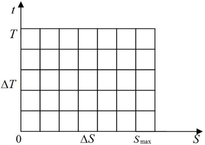
The option price solving diagram
The point (i, j) corresponds the time point j∆T and stock price i∆S, and Vij denotes the option price at point (i, j). For points inside the grid, there are
Substituting (2), (3) and (4) into equation (1) (note that S = i∆S) yields
where
(5) denotes the Crank-Nicolson form of numerical solution of option pricing model with transaction costs. We can rewrite (5) it in matrix form as follows:
Since the cash flow of American put option is max{X – S(T), 0} at time T, we can easily find
Combining (6) with (5) yields the solving equation boundary with initial conditions. That is,
where i = 1, 2, · · · , N, j = 1, 2, · · · , M.
Since the option price at time M∆T can be solved from (6), substituting this result into (7) at time (M – 1)∆T yields
We can solve Vi,M–1, i = 1, 2, ···, N – 1 from (7) and (8). Then comparing Vi,M–1 with X – i∆S. If Vi,M–1 < X – i∆S, the best option is to implement option at time (M – 1)∆T. This implies Vi,M–1 equals X – i∆S. According to the same method, the American option price Vi,0, i = 1, 2, · · ·, N – 1 can be solved. In all of these values, there is an option price is required. In general, it takes a lot of time to use time steps and space steps to get reasonable estimate of the option price. In order to make the values of M and N small as far as possible, we will use the controlling variable technology. In particular, it is to use finite difference method to calculate the American put option price VA and the corresponding price of European put option VE, and also use the Black-Scholes formula to calculate the price of European put option VBS[14]. Finally, American put option price is estimated as VA + VBS – VE using the controlling variable technology.
3 Empirical research
3.1 The selection of data
As of Jan. 31, 2013, Hong Kong Exchanges and Clearing Limited (HKEx) launched 65 Hong Kong stock options. In this paper we select 1 month, 2 months and 5 months of American stock option (CKH) issued by Cheung Kong (Holdings) Limited as the research object. Its underlying stock is Cheung Kong Holdings (00001). The data used is from the website of Hong Kong Exchanges and Clearing Limited.
3.2 The estimate of volatility
Choosing a total of 247 trading days’ closing price data of Cheung Kong Holdings (00001) from Jan. 1, 2012 to Dec. 31, 2012 as estimation samples, estimate the historical volatility of stock returns of the contract period.
To calculate the volatility of stock price, set
where S is the daily closing price, i = 1, 2, · · ·, n, σE is the standard deviation of stock returns within each contract period and τ denotes the number of sample days of contract period. The calculation results obtained by MATLAB language programming are shown in Table 1.
Volatility of stock returns within the contract period
| Stock code | Stock name | Daily Volatility | Volatility | ||
|---|---|---|---|---|---|
| 1 month | 2 months | 5months | |||
| 00001 | Cheung Kong | 0.015298 | 0.068415 | 0.096753 | 0.15298 |
3.3 The estimate of risk-free interest rate
Risk-free interest rate refers to the an ideal investment gains obtained from the capital invested in an item without any risk. In Hong Kong, the risk-free interest rate is usually refers to HIBOR (Hong Kong interbank offered rate). As the duration of the American option of this paper is 1 month, 2 months and 5 months respectively, the corresponding HIBOR rates for 1 month, 2 months and 5 months on January, 31, 2013 as shown in Table 2 are selected.
HIBOR rates for different periods
| date | HIBOR rate(%) | ||
|---|---|---|---|
| 1 month | 2 months | 5months | |
| 01.31.2013 | 0.22786 | 0.33786 | 0.44857 |
3.4 Example analyses
We take the CKH option on January 2, 2013 for example. Its contract period is 1 month, and the price is 150 (HKD). When calculating the theoretical price of HK stock option, the stock price is the closing price of the underlying stock on the trading day. By comparison, take the maximum Smax = 150(HKD), historical volatility σE = 0.068415, the risk free rate r = 0.22786%, the transaction cost k = 0.3% and contract period 1/12, 2/12 and 5/12 respectively.
Using the above data, three values of α respectively corresponding to the lognormal model (α = 1), square root model (α = 0.5) and absolute model (α = 1) represent their impact on the option price. Table 3 shows the resulting option price on January 2, 2013 using different steps M and N by MATLAB language programming.
HK stock option prices using different time and space steps [Unit: (HKD)]
| N | |||||||||
|---|---|---|---|---|---|---|---|---|---|
| M | α = 0 | α = 1/2 | α = 1 | ||||||
| 100 | 200 | 300 | 100 | 200 | 300 | 100 | 200 | 300 | |
| 100 | 28.212 | 29.857 | 31.248 | 29.448 | 30.652 | 31.407 | 32.147 | 33.853 | 36.254 |
| 150 | 29.535 | 31.061 | 32.164 | 30.373 | 31.291 | 31.819 | 33.549 | 35.059 | 36.155 |
| 200 | 30.778 | 31.982 | 32.785 | 30.919 | 31.652 | 32.175 | 34.751 | 35.961 | 36.763 |
Thus, the estimate of Hong Kong option price on January 2, 2013 is obtained. We can see that as time step length and price step length decreases, and stock price option prices gradually convergence and tend to be stable. Actually by the analysis principle of numerical solution of partial differential equation, although it takes a lot of time and calculation to solve a linear equations with a big order in each layer of the finite difference method, format is very stable. When α = 1/2, M = 200, N = 300, the convergence effect of the option price is very good. Therefore, in this paper we select α = 1/2, M = 200, N = 300 as model parameters.
By modifying parameters in M file that has been written in MATLAB software, we deal with financial data of the Cheung Kong Holdings to get the estimated option price from Jan. 1, 2013 to Jan. 15, 2013 (10 days). The results are shown in Table 4.
The theoretical and actual prices of CKH option [Unit: (HKD)]
| Date | 1 month | 2 months | 5 months | |||
|---|---|---|---|---|---|---|
| theoretical | actual | theoretical | actual | theoretical | actual | |
| Jan 2, 2013 | 32.18 | 28.20 | 33.64 | 28.23 | 36.40 | 31.13 |
| Jan 3, 2013 | 33.80 | 29.60 | 35.32 | 29.61 | 38.16 | 32.49 |
| Jan 4, 2013 | 32.52 | 24.50 | 33.84 | 29.11 | 36.72 | 32.00 |
| Jan 7, 2013 | 30.54 | 26.50 | 31.95 | 26.58 | 34.62 | 29.69 |
| Jan 8, 2013 | 30.79 | 27.60 | 32.39 | 27.63 | 34.91 | 30.65 |
| Jan 9, 2013 | 28.90 | 25.30 | 30.25 | 25.37 | 32.83 | 28.44 |
| Jan 10, 2013 | 25.59 | 22.90 | 26.82 | 23.00 | 29.18 | 26.30 |
| Jan 11, 2013 | 27.25 | 24.10 | 28.55 | 24.20 | 31.01 | 27.39 |
| Jan 14, 2013 | 25.32 | 22.61 | 26.33 | 22.79 | 28.81 | 26.16 |
| Jan 15, 2013 | 25.15 | 22.32 | 26.14 | 22.51 | 28.57 | 25.89 |
To analyse the error between theoretical and actual prices of CKH option, we take two metrics: average relative percentage error (RPE) and average absolute percentage error (ARPE). The two measures can be used to measure the deviation of model, but the former is more focused on measuring systematic bias, judging model of pricing is overvalued or undervalued, while the latter can measure either the pricing deviation or pricing efficiency.
Combined with the result of Table 4, we calculate the average relative percentage error and average absolute percentage error according to the different classification of CKH expiration period. Because the two indicators of the calculation results are exactly the same, the only lists the average relative percentage error are shown in Table 5.
The average relative percentage error of different expiration periods (%)
| Date | 1 month | 2 months | 5 months |
|---|---|---|---|
| Jan 2, 2013 | 14.114 | 16.929 | 19.164 |
| Jan 3, 2013 | 14.189 | 17.452 | 19.284 |
| Jan 4, 2013 | 32.735 | 14.750 | 16.249 |
| Jan 7, 2013 | 15.242 | 16.605 | 20.203 |
| Jan 8, 2013 | 11.558 | 13.899 | 17.228 |
| Jan 9, 2013 | 14.229 | 15.436 | 19.235 |
| Jan 10, 2013 | 11.747 | 10.951 | 16.609 |
| Jan 11, 2013 | 13.071 | 13.217 | 17.975 |
| Jan 14, 2013 | 11.986 | 10.130 | 15.533 |
| Jan 15, 2013 | 12.679 | 10.352 | 16.126 |
| RPE | 15.155 | 13.972 | 17.761 |
From the Table 5, we find that average relative percentage error of CKH option price for a month is 32.735% on Jan. 4, 2013, on which day its share price compared to the previous two days did not fluctuate wildly, but the real option price is low. This lead to a higher theoretical option price determined by the stock price relative than the real option price. If we get rid of the calculation result on Jan. 4, 2013, the RPE value of CKH options for 1 month is 13.201%. Therefore, we can think that the pricing efficiency of the CEV model becomes low by the extension of expiration time.
According to the results of Table 4, we use least squares method to fit theoretical and actual prices of different expiration periods respectively. The comparison results are shown in Figure 2 below.
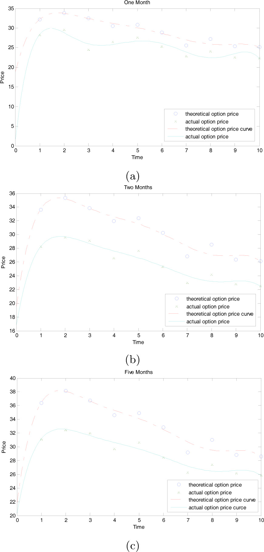
Theoretical and actual option prices curves of different expiration periods
From the images of the fitting and error results we can see that there are certain errors between theoretical and actual prices calculated by CEV model with transaction cost, to a certain extent, close to and have the same trend of fluctuations. It is worth to note that the theoretical and actual prices are close to a certain extent, and have the same trend of fluctuations. It is clear that the American option pricing model under the CEV process with transaction costs has the rationality.
4 Main conclusion
As the application of American option pricing theory, this paper select nearly 1 year’s daily closing price of Hong Kong CKH stock option to calculate the theoretical option prices from January 1 to January 15, 2013 (10 trading days). By comparing analyses between the theoretical and actual prices, the results show that:
(1) The theoretical option price calculated by CEV model is slightly higher than the actual prices. In combination with the practical situation of Hong Kong options market, the causes of overvalued theoretical price is mainly that Hong Kong exchanges and clearing limited continuously introduce new options. The adequate supply and the rich variety not only met the needs of local investors, but also attracted a large number of mainland and overseas investors. In this case, the launch of the new option will not be in higher money demand. In relatively ample supply environment, caused the current actual situation of the stock option price low. The environment of relative enough supply bring the current actual situation of the low price of stock option.
(2) The pricing efficiency of model decreases with the extension of contract period. Average relative percentage error for 1 month is the lowest, at 13.201%, and for 5 months period is largest, to 17.761%. This is because the selected three important parameters in the model (historical volatility and risk-free interest rate and stock price) only reflect the reality of the market situation recently. Over the long term, the stock price may be rise, which lead to actual option prices have a downward trend, but the parameters selected do not reflect the long-term characteristic of realistic economy. Thus, the option pricing error for a long term contract period increases.
(3) Comparing the theoretical and actual prices, we find they are close to a certain extent, and have the same trend of fluctuations. The main factor of price fluctuation of the options is the underlying stock price volatility. It means that the fluctuations of actual prices of CKH is closely related to the fluctuations of its underlying stock (00001) prices. At the same time this verifies the rationality of American option pricing method under the CEV process with transaction costs.
5 Several suggestions on promoting benign development of mainland of China’s stock option market
Fully analyzing the advanced experience of the Hong Kong stock option market and understanding its development situation has important significance to the development of mainland of China’s stock option market.
Based on the conclusion of this paper and in view of the present situation of Hong Kong market, we make three suggestions on the products of stock options that are going to be launched in mainland of China:
(1) Improve the balance of supply and demand mechanism and pay attention to the diversification of option products to meet the needs of different types of investors.
(2) Introduce the market maker system to make a flowing and stable option market.
(3) Improve and develop the stock market to let stock prices linked to enterprise performance, truly reflect the business situation. The implementation of stock option depends on the impartial, fair and reasonable system of the stock market.
References
[1] Hodges S, Neuberger A. Optimal replication of contingent claims under transaction costs. The Review of Futures Markets, 1989, 8(2): 222–239.Suche in Google Scholar
[2] Davis M H, Panas V G, Zariphopoulou T. European option pricing with transaction costs. SIAM Journal of Control and Optimization, 1993, 31(2): 470–493.10.1109/CDC.1991.261597Suche in Google Scholar
[3] Clewlow L, Hodges S. Optimal delta-hedging under transactions costs. Journal of Economic Dynamics and Control, 1997(21): 1353–1376.10.1016/S0165-1889(97)00030-4Suche in Google Scholar
[4] Damgarrd A. Utility based option pricing with proportional transation costs. Journal of Economic Dynamics and Control, 2003, 27(4): 667–700.10.1016/S0165-1889(01)00068-9Suche in Google Scholar
[5] Damgarrd A. Computation of reservation prices of options with proporitional transaction costs. Journal of Economic Dynamics and Control, 2006, 30(3): 415–444.10.1016/j.jedc.2005.03.001Suche in Google Scholar
[6] Monoyios M. Option pricing with transactions costs using a markov chain approximation. Journal of Economic Dynamics and Controls, 2004, 28(5): 889–913.10.1016/S0165-1889(03)00059-9Suche in Google Scholar
[7] Cox J C, Rubinstein M. Options markets. Prentice-Hall, Englewood Cliffs, NJ, 1985.Suche in Google Scholar
[8] Wu Y, He J M. Study on solution of geometric Asian option pricing model under the CEV process. Systems Engineering — Theory & Practice, 2003(4): 32–36.Suche in Google Scholar
[9] Du X Q, Ding H. Numerical solution for binary option following constant elasticity of variance model. South China Journal of Economics, 2006, 19(2): 22–23.Suche in Google Scholar
[10] Qin H Y, Zheng Z L. Option pricing with transaction costs under CEV model. South China Journal of Economics, 2007(9): 38–45.Suche in Google Scholar
[11] Yuan G J, Shi M H. Study on the option pricing model with the proportional transaction cost in the CEV process. Journal of Hefei University of Technology, 2009, 32(10): 1623–1626.Suche in Google Scholar
[12] Etheridge A. A course in financial calculus. Beijing: Posts & Telecom Press, 2006: 82–89.Suche in Google Scholar
[13] Li R H. Numerical solution of partial differential equation. Beijing: Higher Education Press, 2005: 124–128.Suche in Google Scholar
[14] Zhang D F, Cui X Z, Zhao J E. Numerical value method on American put option. Journal of Lanzhou University, 2009, 45(2): 104–106.Suche in Google Scholar
© 2014 Walter de Gruyter GmbH, Berlin/Boston
Artikel in diesem Heft
- Spatial Dynamics, Vocational Education and Chinese Economic Growth
- The Differential Algorithm for American Put Option with Transaction Costs under CEV Model
- Nonlinear Dynamics of International Gold Prices: Conditional Heteroskedasticity or Chaos?
- Design and Pricing of Chinese Contingent Convertible Bonds
- A Robust Factor Analysis Model for Dichotomous Data
- Non-linear Integer Programming Model and Algorithms for Connected p-facility Location Problem
- Uncertain Comprehensive Evaluation Method Based on Expected Value
- MSVM Recognition Model for Dynamic Process Abnormal Pattern Based on Multi-Kernel Functions