Systematic calculations of energy levels and transitions rates in Mo XXVIII

1 Introduction

The concentration of impurities in the plasma and their radiated power through line emission inside the radius of the limiter or the magnetic separatrix are of great concern for tokamak fusion physics devices [1]. The molybdenum content in the plasma was of great concern because their radiation could cause problems in attaining the highest performing pure plasmas [2]. In laser-produced plasma light sources used in the soft X-ray and extreme ultraviolet (EUV) spectral regions, targets of various elements are used to produce suitable wavelengths for specific applications [3]. The selection of target element (Mo) is also critical to maximize emission in the water-window soft X-ray spectral region to develop the most efficient sources for biomedical microscopy and cell tomography [4]. The laser-produced Mo plasma have been provided data for opacity, which is crucial to energy transport by radiation in hot-dense plasma, astrophysics, inertial confinement fusion, and other high energy density physics domains [5]. These applications need a large amount of atomic data to describe the different ionization degree of molybdenum. But for P-like Mo, radiative data have only been published from few works.

In the experimental front, few lines of Mo XV-XXXIII were observed from a spark spectrum by Scheob et al. [6]. A number of spectrum lines arising from magnetic dipole transitions in the 3s^x3p^y (x = 1, 2, and y = 1, 2, 3, 4, 5) configurations in elements 29 ≤ Z ≤ 42 have been observed in the Princeton Large Torus (PLT) tokamak discharges by Denne et al. [7]. The energy-level structure of the 3s²3p³ configurations of Mo XXVIII were determined from magnetic-dipole line wavelengths and emissivities measured in the PLT by Denne et al. [8]. Relative intensity measurements of various lines pairs resulting from magnetic-dipole transitions within the configurations 3s²3p³ were presented by Denne and Hinnov [9]. Transitions of the types 3s²3p^k–3s3p^k+1 and 3p^k–3p^k−13d were identified by Finkenthal et al. in spectra of Mo from PLT tokamak [10]. Phosphoruslike spectra of Mo XXVIII were obtained with the tokamak plasams in the wavelength range of 83 to 163 Å by Sugar et al. [11]. The classification of 15 new n = 3, ∆n = 0 transitions in Mo XXVIII were made by Jupén et al. [12]. Spectra of Mo were investigated by Chowdhuri et al. with the large helical device plasmas [13].

In the theoretical front, calculations based on a simple shell solution for Mo XXVIII were done by Carlson et al. [14]. Scaled Hartree–Fock radial integrals were used by Sugar and Kaufanm in calculating the energy levels of the 3s²3p³ configurations of Molybdenum [15]. The multiconfiguration Dirac–Fock technique was used to calculate energy levels of P-like sequences by Huang [16]. The Hartree–Fock–Slater method was used to energy levels and wavelengths in Mo XX- Mo XL by Câmpecanu et al. [17].

New computations can match measurement, fill gaps, and suggest revisions closely with almost spectroscopic accuracy, which is a critical assessment of theoretical calculations of structure and transition probabilities from the experimenter’s view conducted by Träert [18]. These theoretical citations as well as the ones for experimental data are certainly incomplete. Previous calculations were a number of P-like ions calculations, and the attention was paid to the trend. Limited sets of configurations were discussed [14], [15], [17], or the results were given in the form of diagram [16]. A complete and consistent data set is in demand due to their importance in calculating accurate radiative transition probabilities, which was proved in Al-like Mo calculated by Hu et al. [19]. In some cases, especially when strong self-absorption effects exist, corresponding results for forbidden transitions, such as magnetic dipole (M1), electric quadrupole (E2), and magnetic quadrupole (M2) transitions, are also necessary for modeling and diagnostics of plasmas [1].

In the present work, the multiconfiguration Dirac–Hartree–Fcok method is performed to report energies, E1, M1, E2, and M2 radiative transition properties for Mo XXVIII using the new version of GRASP2018 [20]. Based on our previous work [21], [22], in this paper, the valence–valence (VV) and core-valence (CV) correlation effects are considered in a systematic way. Breit interactions and quantum electrodynamics (QED) effects have been added. This computational approach enables us to present a consistent and improved data set of all important E1, M1, E2, and M2 transitions of the Mo XXVIII spectra, which are useful for identifying transition lines in further investigations.

2 Method

3 Results and discussion

The energies for the low-lying 41 levels of 3s²3p³, 3s3p⁴, and 3s²3p²3d configurations of Mo XXVIII were listed in Table 1. Also listed in this Table 1 are the experimentally complied values of the National Institute of Standards and Technology (NIST) [28]. The NIST database listed the energies for the nine out of the present 41 excited levels in Mo XXVIII. The principal number in this calculation was set to n ≤ 7. There are two reasons for this. One is the convergence as mentioned above. For VV calculation, it is not very difficult to get convergence for higher principal number (n8), but for CV calculation the convergence is difficult. The number of CSFs would increase very rapidly when we include the n ≥ 8 orbitals, and it is hard to get convergence. Also, because of the computer calculation limit and the problem of the program GRASP2K code itself, we only compare the VV and CV models on an equal footing (n ≤ 7), as mentioned above. The other is the contribution from n = 7 less than 0.001%. Figure 1 shows the mean (with the standard deviation) of the relative differences between VVn and NIST is −166 and 5645 cm⁻¹. The smallest difference is 990 cm⁻¹ lower than NIST (3s2 3p3(D32) D3/2o2), and the biggest difference can be up to 9270 cm⁻¹(3s2 3p2(P23) P3 3dF5/22 ). Figure 2 shows the mean (with the standard deviation) of the relative differences between CVn and NIST is 53 and 1625 cm⁻¹. This can be treated as a good example of calculations with the necessary correlations included. As can be seen from Figure 1 and Figure 2, some results considering more configurations are not better than those with fewer configurations. This can be due to configuration mixing, which will be discussed later.

Figure 1:

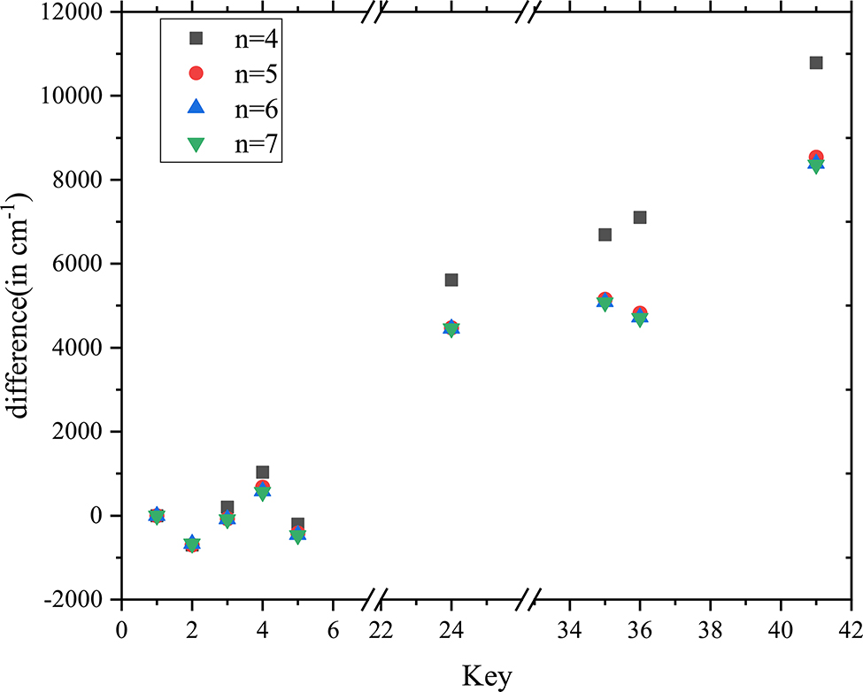
Energy difference between the valence-valence correlation results and the energies for the nine out of the lowest 41 levels from NIST.

Figure 2:

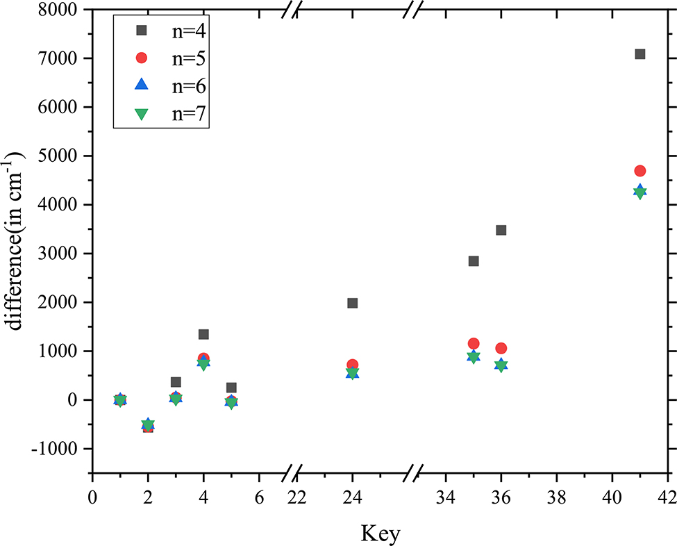
Energy difference between the Core-valence correlation results and the energies for the nine out of the lowest 41 levels from NIST.

The corrections due to Breit interaction and QED to the excited levels of Mo XXVIII are shown in Figure 3. Self-energy and vacuum polarization are the two major components in the QED correction [29]. As can be seen, the contribution of Breit interaction is about 1.12 ∼ 1.83% for 3s²3p³ and 0.09 ∼ 0.86% for 3s3p⁴ and 3s²3p²3d levels, and the contribution of QED is −0.47 ∼ −0.19% for 3s²3p³ and −0.25 ∼ 0.02% for 3s3p⁴ and 3s²3p²3d levels. The excited energy levels of Mo XXVIII are all reduced by the mean value 0.57% due to the inclusion of the Breit interaction and QED corrections. Normal mass shift (NMS) and specific mass shift (SMS) are also included in this calculation. The contribution of NMS for 3s²3p³ is about −0.001%, while −0.0001% for 3s3p⁴ and 3s²3p²3d levels. The contribution of SMS for 3s²3p³ is about 0.002% and −0.001% 3s3p⁴ and 3s²3p²3d levels. So, the contribution of NMS and SMS was not plotted in Figure 3.

Figure 3:

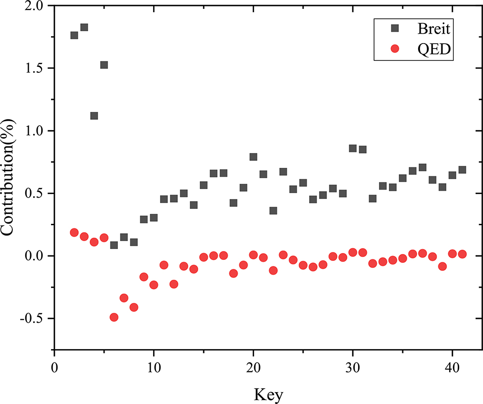
The effect of the Breit interaction and QED corrections on the excitation energies of the Mo XXVIII configurations obtained from the present MCDHF calculations.

The data from VV and CV calculations are compared with the energies from qusairelativistic Hartree–Fock plus configuration interactions given by Applicable Data of Many-electron Atom energies and Transitions (ADAMANT) [30] in Figure 4. The present results in Figure 4 are VV and CV calculations with n = 7. For 3s²3p³, the VV results agree well with NIST in the range of −0.42 to 0.21%, while CV in the range of −0.31 to 0.29%. For 3s²3p²3d, the VV results agree well with NIST in the range of 0.33 to 0.55%, while CV in the range of 0.04 to 0.28%. The results from ADAMANT are in general agreement with NIST. The difference of 3s2 3p2(P23) P3 3d F5/22 between NIST and theoretical results can up to 0.68%, which was dubious. This is because all the theoretical results were estimated. And the result of NIST corresponds to the 3s2 3p2(P23) P3 3dD5/22 is 150,8720 cm⁻¹, while theoretical result is about 127,0000 cm⁻¹. The identification of experimental results is very difficult. The previous results from Jupén et al. [12] were not adopted by NIST. For example, the difference between 3s2 3p2(D21) D1 3dD3/22 and 3s2 3p2(D21) D1 3dD5/22  is up to about 15,4000 cm⁻¹ [12], while theoretical result is only about 1000 cm⁻¹.

Figure 4:

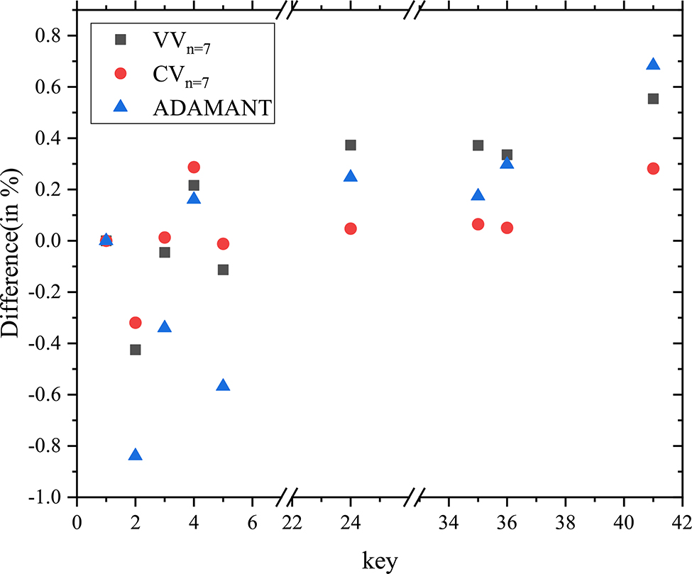
Difference (in %) of various theoretical energies from the NIST complied values in Mo XXVIII.

Dirac–Fock wave functions with a minimum number of radial functions are not sufficient to represent the occupied orbitals. Extra configurations have to be added to adequately represent electron correlations. These extra configurations are represented by CSFs and must have the same angular momentum and parity as the occupied orbitals, which cause a problem in identifying the accurate term for each state. For example, the configuration-mixed wave function for the 3s2 3p3(S34) S∘3/24 level is represented as 3s2 3p3(S34) S∘3/24=0.47 3s2 3p3(S34)S∘4+0.343 s2 3p3(P12)P∘2 +0.18 3s2 3p3(D32) D∘2, where 0.47, 0.34 are 0.18 are contributions. The most important contributions to the total wave function of a given level are those from the major configurations. Clearly, the present VV and CV results are in a general agreement. But the order of 3s2 3p2(P23) P3 3d P1/22, 3s2 3p2(P23)P3 3d P1/24, and 3s S2 3p4(S01) S1/22 levels is different between VV and CV calculations. This is due to more complex system, which it sometimes happens that two or even more level have the same dominating LS term. These three levels get the same quantum labels in present calculations. The GRASP2018 procedure JJ2LSJ [31] was used to transform ASFs from a jj-coupled CSF basis [32] into an LSJ-coupled CSF basis and select the dominate LS term for the results. With the help of JJ2LSJ, the levels 3s S2 3p4(P23) P3/22, 3s2 3p2(D21) D1 3d G7/22, 3s S2 3p4(P23) P1/22, and 3s2 3p2(D21) D1 3d P1/22 have been adjusted in this calculation. In the present calculations, the nuclear parameters I, μI, and Q are all set to 1. The AJ and BJ values for a specific isotope can be scaled with the tabulated values given from Table 2.

Among the calculated wavelengths of transition between the lowest 41 levels in Mo XXVIII, the experimental data compiled by NIST listed the observed wavelengths for four E1 transitions and six M1 transitions. The observed results are from Denne et al. [8] and Sugar et al. [11]. Also, the wavelengths from Jupén et al. [12], which were not compiled by NIST. The accuracy of calculated CV and VV wavelengths relative to experimental results can be assessed from Table 3, where the agreement is within 0.07 Å for CV calculation except the transition 3sS2 3p4(P23) P3/24−3s 2 3p3(S34) S3/2o4 with a calculated wavelength λ = 84.771 Å deviates from the measure by about 0.21 Å. The difference between VV and observed results is in the range of −0.09 ∼ −0.49 Å. The wavelength of 3s2 3p2(P23) P3 3d P3/24−3s2 3p3(P12) P3/2o2 (not listed in Table 3) adopted by NIST is 91.301 Å, which corresponding to the transition 3s2 3p2(P23) P3 3d P3/24−3s2 3p3(P12) P3/2o2 in CV and VV calculation. The differences between CV and experimental results are in the range of −0.012 ∼ −0.213 Å for E1 transitions and −0.58 ∼ 2.96 Å for M2 transitions. The VV results are in the range of −0.098  ∼ −0.493 Å for E1 and −1.27 ∼ −2.94 Å for M2. The result of M2 transition 3s2 3p3(D32) D3/2o2−3s2 3p3(S34) S3/2o4 is overestimated about 26 Å.

Lifetime is a measurable datum, and it can be a good check on the accuracy of present calculation [22]. Lifetimes for the lower 36 levels in Mo XXVIII in length and velocity are listed in Table 4. Contributions from all possible E1 and M2 radiative decays are included in lifetimes, and dominated by E1 transitions. The value τl/τv for CV calculations is in range of 0.923 ∼ 1.093, while 0.960 ∼ 1.196 for VV calculations. To assess the accuracy of these theoretical results, the ratios of CVτl/VVτl and VVτv/VVτv are also listed in Table 4. The mean ratio of CVτl/VVτl is 1.021 and 1.051 for VVτv/VVτv. Lifetimes of 3s2 3p2(P23) P3 3d F9/24 and 3s2 3p2(D21) D1 3d G9/22 are 0.176 and 1.389 ms, which are very stable and can be measured in the future.

The transition rate, the weighted oscillator strength and the line strength were given in Coulomb (velocity) and Babushkin (length) gauges in this calculation. Also, for the electric transitions the relative difference (dT) (dT=abs(Al−Av)/max(Al/Av)) between the transition rates in length and velocity gauges are given. A value close to dT = 0 for an allowed transition is a known accuracy indicator [33]. In many cases the values are reasonably close to zero, see Figure 5. But in other cases, for example, the difference of transition 3s S2 3p4(D21) D3/22−3s2 3p3(P12) P3/2o2 can be larger than 0.455. In particular, these calculations presented provide comprehensive new data for E2, M1, and M2 transitions for Mo XXVIII, which no existent data for public. This will help with the identification of spectral lines of Mo XXVIII. Owing the space limitations, full tables of E1, E2, M1, and M2 transitions data will be provided as the supplemental material in conjunction with the E-mail.

Figure 5:

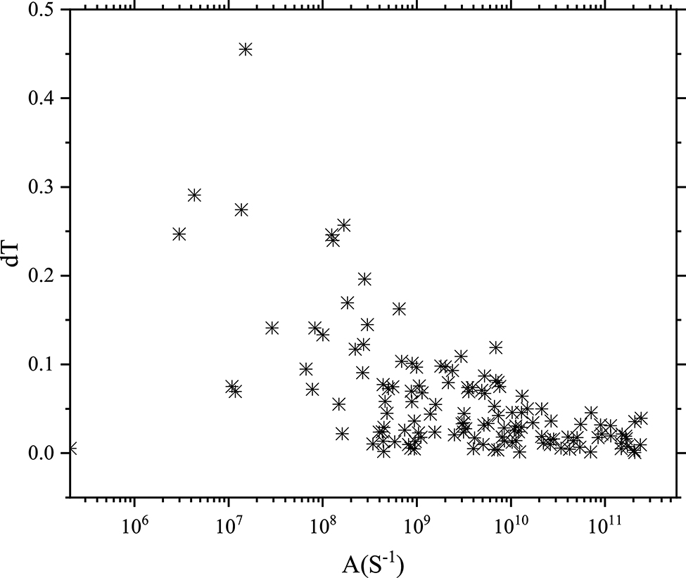
Scatterplot of dT and A (S⁻¹) for all E1 transitions.

4 Conclusions

Using the MCDHF methods with considering the electron correlations, energy levels, lifetimes, wavelengths, hyperfine structures, Landé g_J-factors and E1, E2, M1, and M2 line strengths, oscillator strengths, transitions rates are reported for the low-lying 41 levels belonging to the 3s²3p³, 3s3p⁴, and 3s²3p²3d configurations of P-like Mo XXVIII have been determined. The accuracy of energy levels and transition probabilities is estimated by comparing VV and CV results with available theoretical and experimental data. Excitation energies are accurate to within 0.04%. The computed wavelengths are almost spectroscopic accuracy, aiding line identification in spectra. Our results are useful for many applications such as controlled thermonuclear fusion, laser and plasma physics as well as astrophysics.

References

[1] M. J. May, M. Finkenthal, S. P. Regan, et al., “The measurement of the intrinsic impurities of molybdenum and carbon in the Alcator C-Mod tokamak plasma using low resolution spectroscopy,” Nucl. Fusion, vol. 37, p. 881, 1997, https://doi.org/10.1088/0029-5515/37/6/i13.Search in Google Scholar
[2] D. M. Meade, “Effect of high-Z impurities on the ignition and Lawson conditions for a thermonuclear reactor,” Nucl. Fusion, vol. 14, p. 289, 1974, https://doi.org/10.1088/0029-5515/14/2/017.Search in Google Scholar
[3] T. Tamura, G. Arai, Y. Kondo, et al., “Selection of target elements for laser-produced plasma soft x-ray sources,” Opt. Lett., vol. 43, p. 2042, 2018, https://doi.org/10.1364/ol.43.002042.Search in Google Scholar
[4] T. Tamura, G. Arai, Y. Kondo, et al., “Soft X-ray emission from molybdenum plasmas generated by dual laser pulses,” Appl. Phys. Lett., vol. 109, 2016, Art no. 194103. https://doi.org/10.1063/1.4967310.Search in Google Scholar
[5] B. Qing, Z. Y. Zhang, M. X. Wei, et al., “Opacity measurements of a molybdenum plasma with open M-shell configurations,” Phys. Plasmas, vol. 25, 2018, Art no. 023301. https://doi.org/10.1063/1.5012695.Search in Google Scholar
[6] J. L. Schwob, M. Klapisch, N. Schweitzer, et al., “Identification of Mo XV to Mo XXXIII in the soft X-ray spectrum of the TFR Tokamak,” Phys. Lett. A, vol. 62, p. 85, 1977, https://doi.org/10.1016/0375-9601(77)90957-4.Search in Google Scholar
[7] B. Denne, E. Hinnov, S. Suckewer, S. Cohen, “Magnetic dipole lines in the 3s23px configurations of elements from copper to molybdenum,” Phys. Rev. A, vol. 28, p. 206, 1983, https://doi.org/10.1103/physreva.28.206.Search in Google Scholar
[8] B. Denne, E. Hinnov, S. Suckewer, J. Timberlake, “On the ground configuration of the phosphorus sequence from copper to molybdenum,” J. Opt. Soc. Am. B, vol. 1, p. 296, 1984, https://doi.org/10.1364/josab.1.000296.Search in Google Scholar
[9] B. Denne, E. Hinnov, “Spectrometer-sensitivity calibration in the extreme ultraviolet by means of branching ratios of magnetic-dipole lines,” J. Opt. Soc. Am. B, vol. 1, p. 699, 1984, https://doi.org/10.1364/josab.1.000699.Search in Google Scholar
[10] M. Finkenthal, B. C. Stratton, H. W. Moos, et al., “Spectra of highly ionised zirconium and molybdenum in the 60-150 AA range from PLT tokamak plasmas,” J. Phys. B, vol. 18, p. 4393, 1985, https://doi.org/10.1088/0022-3700/18/22/009.Search in Google Scholar
[11] J. Sugar, V. Kaufman, W. L. Rowan, “Spectra of the P i isoelectronic sequence from Co XIII to Mo XXVIII,” J. Opt. Soc. Am. B, vol. 8, p. 22, 1991, https://doi.org/10.1364/josab.8.000022.Search in Google Scholar
[12] C. Jupén, B. Denne, E. Hinnov, I. Martinson, L. J. Curtis, “Additions to the Spectra of Highly Ionized Molybdenum, Mo XXIV–Mo XXVIII,” Phys. Scripta, vol. 68, p. 230, 2003, https://doi.org/10.1238/physica.regular.068a00230.Search in Google Scholar
[13] M. B. Chowdhuri, S. Morita, M. Goto, et al., “Line analysis of EUV spectra from molybdenum and tungsten injected with impurity pellets in LHD,” Plasma Fusion Res., vol. 2, p. S1060, 2007, https://doi.org/10.1585/pfr.2.s1060.Search in Google Scholar
[14] T. A. Carlson, C. W. Nestor, N. Wasserman, J. D. McDowell, “Calculated ionization potentials for multiply charged ions,” Atomic Data Nucl. Data Tables, vol. 2, p. 63, 1970, https://doi.org/10.1016/s0092-640x(70)80005-5.Search in Google Scholar
[15] J. Sugar, V. Kaufman, “Predicted wavelengths and transition rates for magnetic-dipole transitions within 3s23pn ground configurations of ionized Cu to Mo,” J. Opt. Soc. Am. B, vol. 1, p. 218, 1984, https://doi.org/10.1364/josab.1.000218.Search in Google Scholar
[16] K. -N. Huang, “Energy-level scheme and transition probabilities of P-like ions,” Atomic Data Nucl. Data Tables, vol. 30, p. 313, 1984, https://doi.org/10.1016/0092-640x(84)90020-2.Search in Google Scholar
[17] R. I. Câmpeanu, “HFS energy levels and wavelengths in Mo XX–XL,” Rev. Roum. Phys., vol. 30, p. 307, 1985.Search in Google Scholar
[18] E. Träbert, “Critical assessment of theoretical calculations of atomic structure and transition probabilities: an experimenter's view,” Atoms, vol. 2, no. 1, p. 15, 2014, https://doi.org/10.3390/atoms2010015.Search in Google Scholar
[19] F. Hu, Y. Sun, M. F. Mei, “Fine-structure energy levels and radiative rates in Al-like molybdenum,” Can. J. Phys., vol. 95, p. 59, 2017, https://doi.org/10.1139/cjp-2016-0303.Search in Google Scholar
[20] C. Froese Fischer, G. Gaigalas, P. Jönsson, J. Bieroń, “GRASP2018—A Fortran 95 version of the general relativistic atomic structure package,” Phys. Commun., vol. 237, p. 184, 2019, https://doi.org/10.1016/j.cpc.2018.10.032.Search in Google Scholar
[21] F. Hu, M. F. Mei, C. Han, et al., “Accurate multiconfiguration Dirac–Hartree–Fock calculations of transition probabilities for magnesium-like ions,” J. Quant. Spectrosc. Radiat. Transfer, vol. 149, p. 158, 2014.10.1016/j.jqsrt.2014.08.006Search in Google Scholar
[22] F. Hu, Y. Sun, M. F. Mei, C. C. Sang, J. M. Yang, “Energy levels, radiative rates, and lifetimes for transitions in Fe XIV,” J. Appl. Spectrosc., vol. 85, p. 749, 2018, https://doi.org/10.1007/s10812-018-0715-4.Search in Google Scholar
[23] P. Jönsson, X. He, C. Froese Fischer, I. P. Grant, “The grasp2K relativistic atomic structure package,” Comput. Phys. Commun., vol. 177, no. 7, p. 597, 2007, https://doi.org/10.1016/j.cpc.2007.06.002.Search in Google Scholar
[24] P. Jönsson, G. Gaigalas, J. Bieroń, C. Froese Fischer, I. P. Grant, “New version: Grasp2K relativistic atomic structure package,” Comput. Phys. Commun., vol. 184, no. 9, p. 2197, 2013, https://doi.org/10.1016/j.cpc.2013.02.016.Search in Google Scholar
[25] B. J. McKenzie, I. P. Grant, P. H. Norrington, “A program to calculate transverse Breit and QED corrections to energy levels in a multiconfiguration Dirac-Fock environment,” Comput. Phys. Commun., vol. 21, no. 2, p. 233, 1980, https://doi.org/10.1016/0010-4655(80)90042-9.Search in Google Scholar
[26] K. G. Dyall, I. P. Grant, C. T. Johnson, F. A. Parpia, E. P. Plummer, “GRASP: A general-purpose relativistic atomic structure program,” Comput. Phys. Commun., vol. 55, no. 3, p. 425, 1989, https://doi.org/10.1016/0010-4655(89)90136-7.Search in Google Scholar
[27] I. P. Grant, Relativistic Quantum Theory of Atoms and Molecules, New York, Springer, 2007.10.1007/978-0-387-35069-1Search in Google Scholar
[28] A. Kramida, Atomic Transition Probability Bibliographic Database, Version 9.0, Gaithersburg, MD, National Institute of Standards and Technology, 2019 [Online]. Available at: https://physics.nist.gov/Elevbib [accessed: Oct. 18, 2019].Search in Google Scholar
[29] Y. K. Kim, D. H. Baik, P. Indelicato J. P. Desclaux, “Resonance transition energies of Li-, Na-, and Cu-like ions,” Phys. Rev. A, vol. 44, p. 148, 1991, https://doi.org/10.1103/physreva.44.148.Search in Google Scholar
[30] ADAMANT(Applicable Data of Many-electron Atom energies and Transitions) [Online]. Available at: http://158.129.165.241/ege.php [accessed: Oct. 29, 2019].Search in Google Scholar
[31] G. Gaigalas, C. Froese Fischer, P. Rynkun, P. Jönsson, “JJ2LSJ transformation and unique labeling for energy levels,” Atoms, vol. 5, p. 6, 2017, https://doi.org/10.3390/atoms5010006.Search in Google Scholar
[32] C. Nazé, E. Gaidamauskas, G. Gaigalas, M. Goderfroid, P. Jönsson, Comput. Phys. Commun., vol. 184, p. 2187, 2013, https://doi.org/10.1016/j.cpc.2013.02.015.Search in Google Scholar
[33] J. Ekman, M. R. Godefroid, H. Hartman, “Validation and implementation of uncertainty estimates of calculated transition rates,” Atoms, vol. 2, p. 215, 2014, https://doi.org/10.3390/atoms2020215.Search in Google Scholar
Supplementary Material
The online version of this article offers supplementary material (https://doi.org/10.1515/zna-2020-0119).
© 2020 Walter de Gruyter GmbH, Berlin/Boston
Articles in the same Issue
- Frontmatter
- Atomic, molecular & chemical physics