Multistability Control of Hysteresis and Parallel Bifurcation Branches through a Linear Augmentation Scheme

1 Introduction

Multistability or coexistence of attractors refers to the superposition of several disconnected attractors in a given system for the same set of parameters, starting from different initial conditions [1]. Premises of multiple behavior modes and multiple limit cycles in a nonlinear system were identified in [2] by Ogata and later confirmed in nonlinear electronic circuits by Arecchi and colleagues [3], [4]. In fact, Arecchi et al. reported the switches between coexisting states of low-frequency spectral components in the power spectrum diagrams induced by noise. Since then, multistability did not stop attracting numerous researchers who have continued to publish several papers on that topic [5], [6], [7], [8], [9], [10], [11], [12], [13], [14], [15], [16], [17], [18], [19], [20], [21]. In this scope, new terms/expressions like extreme multistability (i.e. coexistence of an infinite number of attractors for a fixed set of parameters and by varying only initial conditions), megastability (i.e. systems with nested infinite attractors) [22], [23] and hidden attractors (i.e. its basin of attraction does not intersect with small neighbourhoods of equilibria [24]) are now famous and harnessed within existing dynamical systems.

Multistability offers great flexibility in the system performance without major parameter changes with the possibility of switching between different coexisting states. However, the random jump between different coexisting states due to small perturbations may lead to the disastrous performance of the investigated system by spoiling its reliability and reproducibility. This has been observed, for instance, in laser systems where multistability-induced intracavity second harmonic generation leads to the well-known green problem [25]. Also, multistability can often create inconvenience in the design of a commercial device with specific characteristics [26], [27]. Several other examples showing the disadvantages of multistability in real life problems and dynamical systems are well discussed in [28]. All these non-exhaustive drawbacks sufficiently demonstrate the necessity to control multistability or stabilising the multistable system against noisy environments [27], [29]. Several techniques exist in the literature to control multistability (by destroying/annihilating some attractors) or target a specific attractor. We can mention the control method by noise selection [28], short pulses [30], harmonic perturbation [31], pseudo-periodic forcing [32], [33], and linear augmentation [34], [35], [36], [37] just to name a few. Except for the linear augmentation method, in almost all the reported methods, the control is applied to one parameter of the system or the system variable. However, it may not generally be possible to modify the system parameters to remove one of the attractors for all initial conditions. Henceforth, external controls such as the linear augmentation method would be preferred.

Indeed, as its successful application for the first time on the stabilisation of fixed-point solution in chaotic systems was made by Sharma et al. [34], the linear augmentation scheme has been extended later on the control of bistable chaotic attractors comprising a well-separated unstable fixed point [29]. More recently, the same author and colleagues showed the capability of the scheme to obtain the desired output on a unidirectionally coupled drive-response system [36]. In opposition to other methods proposed in the literature on the control of multistability, the linear augmentation scheme presents the following advantages:

1. Very simple to implement.

2. Based on simple decaying function with a decay parameter that can be used to control the time required to stabilise the system at the desired dynamical behaviour.

3. Is external and preferred in the case of inaccessibility of the internal system parameters and/or variables.

Also, the method is suited in the case where one desires to target a specific attractor among several ones in the case of coexistence of multiple attractors [29], [35], [36], [37]. Clearly, the control is a design such that by varying the upward the coupling strength, some of the attractors are annihilated. As a result, the former studied multistable system turns into a monostable one. In this paper, we are applying the linear augmentation scheme to turn the multistable simplified hyperchaotic canonical Chua’s system (marked by the coexistence of five disconnected attractors) to a monostable one. Although a linear augmentation scheme has been applied in systems with self-excited and hidden attractors [29], [34], [35], [36], [38], [39], only bistable cases were investigated. Making the results presented within this work more general and relevant.

The layout of the paper is as follows: Section 2 introduces the circuit realisation of the simplified hyperchaotic canonical Chua’s oscillator (SHCCO) and its equivalent mathematical model. The symmetry property of the model is also discussed. In Section 3, numerical analysis is performed to highlight the complex dynamical behaviours of the SHCCO including chaos, hyperchaos, and multistability with the coexistence of five disconnected attractors. Bifurcation diagrams, the graph of maximum Lyapunov exponent and two-parameter diagrams are exploited to reveal such complex dynamical behaviours. Coexisting attractors are discussed using bifurcation diagrams, phase portraits and basin of attractions as arguments. Brief description of the linear augmentation scheme is further presented in Section 4. Basic properties of the controlled system are also presented. The results and discussions of the multistability control in the SHCCO are then presented Section 5. Finally, in the last section, we present our conclusions and indicate possible further works.

2 Circuit Realisation and its Model

The schematic diagram of the SHCCO is depicted in Figure 1. It consists of four reservoirs (i.e. capacitors C1,2 and inductors L1,2), a negative impedance converter [41] and antiparallel diodes of type 1N4148 which serve as the only nonlinear elements of the whole circuit. Let us remember that the circuit diagram in Figure 1 is a simplified version of that proposed earlier by Thamilmaran and co-authors (made of 13 electronic components within which five are used to implement the piecewise Chua’s nonlinearity) [40] where the nonlinearity has been replaced with antiparallel diodes and henceforth reducing the number of off-the-shelf electronic components to 10. It is found that the proposed SHCCO shows the same scenarios to chaos/hyperchaos as in the work of Thamilmaran et al. [40] but also experiences (not earlier reported) the phenomenon of multistability with the coexistence of three and up to five disconnected attractors in its control bifurcation region (see Section 3), and thus deserve dissemination.

Figure 1:

Schematic diagram of the SHCCO. The Chua’s diode present in [40] has been replaced with switching antiparallel diodes of types 1N4148.

Applying Kirchhoff’s laws to the schematic diagram of Figure 1, a set of four order autonomous differential equations describing the dynamics of the SHCCO is presented in (1).

Here, I_i (i = 1, 2) denotes the current flowing through inductors L_i and by V_j (j = 1, 2) denote the voltage across the capacitors C_j, respectively. For numerical simulation, we normalise the circuit equations (1) with appropriate rescaling parameters as: t=τL2C2; κ=1/nVT; ρ=L2/C2; x1=κV1; x2=κρI1; x3=κV2; x4=κρI2; α1=C2/C1; α2=L2/L1; ε = ρG; γ=2κρIs. Consequently, a set of dimensionless/normalised equations are defined by the following smooth and simple/elegant nonlinear coupled fourth-order autonomous differential equations:

The dimensionless system present in (2) contains only one nonlinear term (i.e. the sine hyperbolic function) in which only one state variable x₁ is involved. Also, in the mathematical model of system (2), four parameters can be identified. Except for γ, all other parameters can serve as bifurcation parameters in other to highlight the complex dynamical behaviour of the SHCCO. Also, system (2) is symmetric around the origin. Indeed, it is invariant under any rotation of 180° of the space (x1,x2,x3,x4) around the origin O(0, 0, 0, 0). So, attractors of the model will appear in asymmetric pairs in the (x1,x2,x3,x4) plane to restore the exact symmetry by using a pair of symmetric initial conditions. Otherwise, the attractors generated will remain symmetric if the exact symmetry of the orbits has already been restored. This method has been widely used recently to track coexisting attractors in symmetric systems [42], [43].

3 Complex Dynamical Behaviours in the SHCCO

From the general theory of nonlinear dynamics, and by setting the right-hand side of (2) to zero, it is found that the origin O(0, 0, 0, 0) is the trivial and the only equilibrium point of the system. Further analysis using the Newton-Raphson algorithm for ε = 0.9873, α1=10.0, α2=10.64516129 and γ=1.32986467×10−4 revealed that the equilibrium point origin O(0, 0, 0, 0) is of unstable nature as it possesses all the eigenvalues with positive real parts (Λ1,2=0.0446±j10.8214;Λ3,4=0.4483±j0.8414). This leads to conclude that the SHCCO can generate self-excited attractors as its basin of attraction is related to an unstable fixed point in opposition to hidden attractors where their basin of attractions do not intersect with small neighbourhoods of any equilibrium points [44], [45].

The computational method applied hereafter consist of integrating system (2) using the fourth-order Runge–Kutta scheme for a sufficiently long time and by discarding a long transient. All the diagrams of bifurcations will be obtained by superposing hysteresis analysis with parallel branches. Clearly, five sets of data will be superimposed. Three of them will belong to hysteresis analysis (i.e. upwards and downwards of the control parameter with the continuation method) and the last computed states are used as initial conditions in the next iteration. The two other sets of data are associated with parallel bifurcation schemes. That is, the system is firstly integrated with fixed initial conditions to highlight regions in the control parameter which predict different bifurcation than that of the hysteresis strategy. Once localised, continuation strategy (i.e. starting integration now with the corresponding initial states which lead to such parallel attractor/branches) is then applied to obtain the whole parallel bifurcation branches. This strategy was recently used to uncover up to five, seven and nine disconnected attractors in several self-excited nonlinear dynamical system including neural networks, Jerk/hyperjerk oscillators and the Moore–Spiegel system just to name few [46], [47], [48], [49].

By setting parameters α2=10.64516129, γ=1.32986467×10−4 and varying upwards parameters (α1,ε)∈[2,14]∪[0.8,1.8], we have plotted in Figure 2 the two-parameters map showing the different dynamical behaviours in the SHCCO through different colours using the reliable algorithm of Wolf et al. [50]. Red and yellow colours are associated, respectively, to hyperchaotic and chaotic dynamics while the cyan colour showsthe region of regular (periodic and quasiperiodic) dynamics. From Figure 2, we have shown the scenarios to hyperchaos along the line L. This is clearly materialised by the two-dimensional (2D) phase diagrams in Figure 3 as a function of ε and for α₁ = 10. One can notice that system (2) undergoes from the period doubling route to quasi-periodic, chaotic and then hyperchaotic attractors (see Fig. 3). The fact that some attractors are appearing in asymmetric ways is a signature of coexisting attractors in the SHCCO [42], [43].

Figure 2:

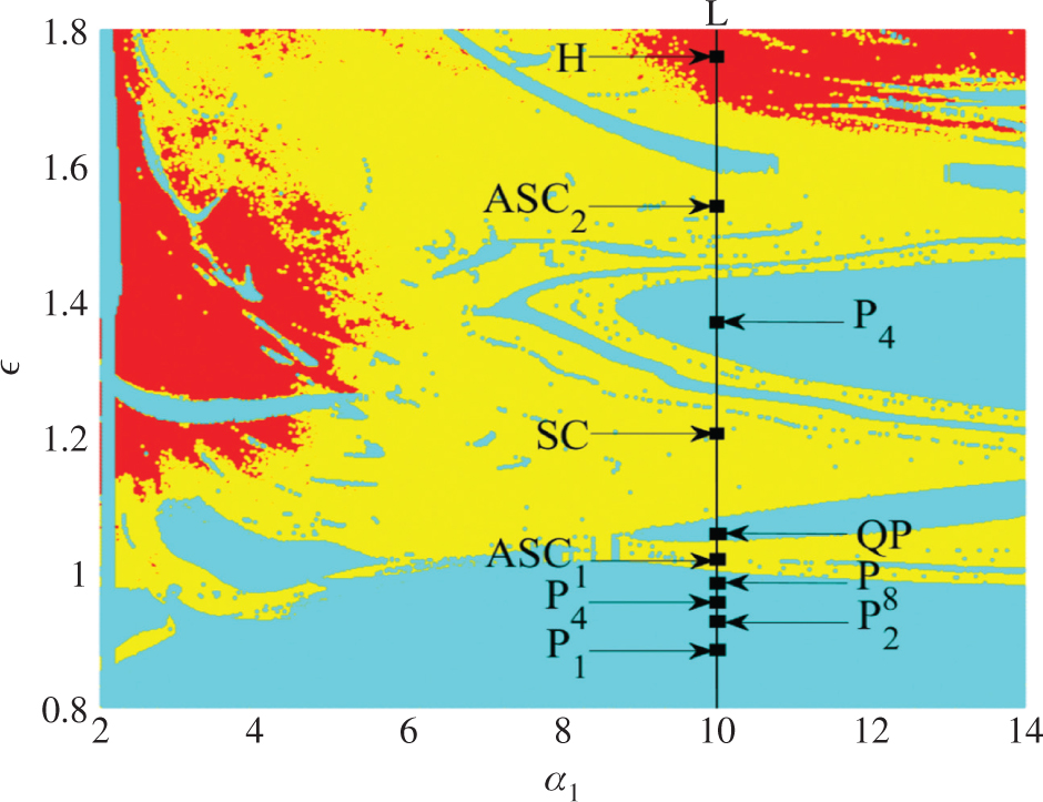
Dynamical map presenting in the two parameters space (α1,ε) the demarcation regions of each dynamical behaviors in the SHCCO. Red and yellow colours are associated, respectively, with hyperchaotic and chaotic dynamics while cyan colour shows regions of regular (periodic and quasiperiodic) dynamics. Line L shows the route to hyperchaos as depicted in Figure 3. 0.8≤ε≤1.8, 2≤α1≤14 and the rest of system parameters are fixed as: α2=10.64516129 and γ=1.329864674×10−4 with X(0) = (0.5, 1.0, 0.5, 0). (For interpretation of the references to colour in this figure legend, the reader is referred to the text).

Figure 3:

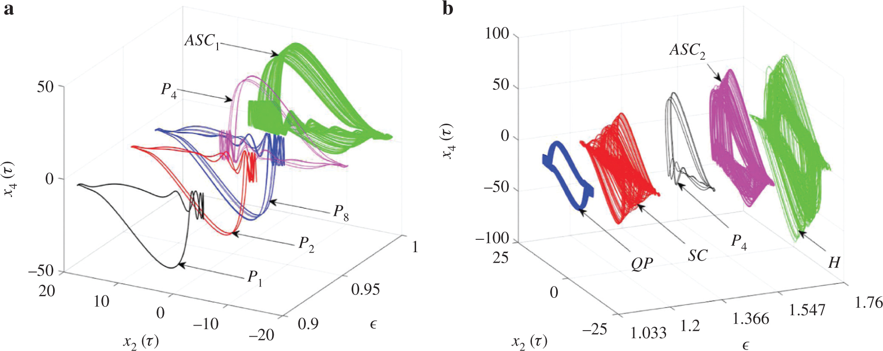
(a) and (b) show the period doubling route to chaos and quasi-periodic route to hyperchaos along the line L in Figure 2 as a function of ε for α₁ = 10. The rest of the parameters are those of Figure 2. Period-1 cycle (P₁) in black colour for ε = 0.9, Period-2 cycle (P₂) in red colour for ε = 0.968, Period-4 cycle (P₄) in magenta colour for ε = 0.964, Period-8 cycle (P₈) in blue colour for ε = 0.947, asymmetric chaotic attractor (ASC₁) in green colour for ε = 1.0, symmetric quasi-periodic attractor (QP) in blue colour for ε = 1.033, symmetric chaotic attractor (SC) in red colour for ε = 1.2, asymmetric period-4 cycle (P₄) in black colour for ε = 1.366, asymmetric chaotic attractor (ASC₂) in magenta colour for .., symmetric hyperchaotic attractor (H) in green colour for ε = 1.76.

This striking phenomenon is confirmed through the bifurcation diagrams and the corresponding largest Lyapunov exponents depicted in Figure 4a,b, respectively. From these diagrams, five different branches are superimposed in other to justify the coexisting bifurcation as well as the hysteretic dynamic in the SHCCO system. These coexisting bifurcation diagrams are obtained when monitoring (i.e. upward and downward strategies) parameter ε in the range [0.98, 0.995] starting from three distinct initial states while keeping α₁ = 10, α2=10.64516129, γ=1.32986467×10−4. Firstly, the data in red and magenta colours are obtained by increasing the bifurcation parameter ε while integrating the SHCCO from the initial state x1(0)=±0.5, respectively. Then, the data in the green colour is produced by integrating system (2) from an initial state x1(0)=1.5. Finally, the bifurcation diagram in black and blue colours are captured by varying upward and downward the bifurcation control parameter ε while integrating the SHCCO from the initial conditions x1(0)=∓0.5, respectively. These later bifurcation diagrams were obtained through parallel branches and continuation techniques [48], [49], [51] while the three formers (green, red and magenta colours) are associated with hysteresis dynamics [16], [52]. The strategy adopted here clearly highlights the symmetry nature of the SHCCO by revealing the number of coexisting attractors on the SHCCO when varying ε in the range [0.98, 0.995]. Clearly, it uncovers a region of dynamics of the SHCCO with the coexistence of five disconnected attractors (i.e. 0.9866 ≤ ε ≤ 0.9878) as depicted by the 2D phase portraits for various initial states in Figure 5a,b. Except from this specified region, the SHCCO still presents the multistability phenomenon but only with the coexistence of three disconnected attractors (i.e. ε ∈ [0.98, 0.9866[∪]0.9878, 0.995]). From Figure 5a,b, the possibility of five different attractors (an asymmetric pair of a chaotic attractor, an asymmetric pair of a period-3 cycle, and a symmetric periodic attractor) in the planes (x1(0),x2(τ),x4(τ)) and (x1(0),x1(τ),x4(τ)) can be observed. To obtain these stable states, we have fixed ε = 0.9873 and we used random initial conditions. That is, the pair of asymmetric chaotic (resp. period-3 cycle) attractor in black and red colours (resp. blue and yellow) are found for x1(0)=±0.5 (resp. x1(0)=±0.1) while the symmetric period-3 cycle attractor (green) is obtained for x1(0)=1.5 with the other initial states set to zero. Demarcation regions (i.e. basin boundary) of the initial states which characterise each of these coexisting solutions are depicted in Figure 5c,d captured in the (x1(0),x2(0)) and (x1(0),x3(0)) planes. We can clearly remark that the space magnetisation is characterised by five different colours which are linked to each of the coexisting attractors (see Fig. 5).

Figure 4:

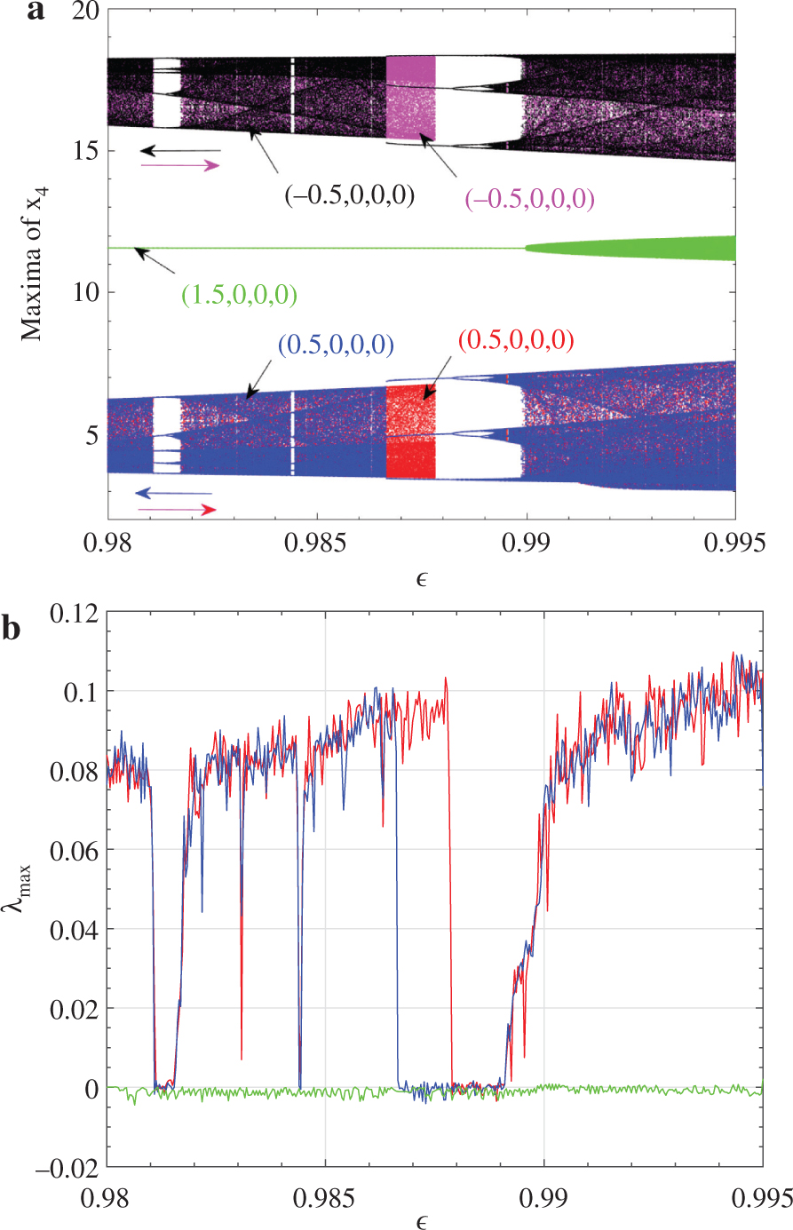
(a) Bifurcation diagrams and corresponding (b) maximum Lyapunov exponents of system (2) showing the superposition of five sets of data when increasing and decreasing the control parameter ε from the three different initial conditions as specified in the diagrams. The bifurcation diagrams in red, magenta and green colours are obtained using the hysteresis method while those in black and blue colours are related to parallel branches. The rest of system parameters are those of Figure 2 with α₁ = 10.

Figure 5:

Five disconnected attractors as a function of initial conditions x1(0) in the planes (a) (x2(τ),x4(τ)) and (b) (x1(τ),x4(τ)), respectively, and corresponding cross section the basin of attraction showing the demarcation initial conditions regions of each coexisting attractors in the planes (c) (x1(0),x2(0)) and (d) (x1(0),x3(0)) for ε = 0.9873 and all other initial conditions fixed as equal to zero. (For interpretation of the references to colour in this figure legend, the reader is referred to the text.)

It ought to be stressed that, to the best of the authors’ knowledge, the striking phenomenon of multiple stability involving up to five disconnected coexisting attractors has not yet been reported in the Chua’s oscillator [53], and thus represents an enriching contribution related to the dynamics of Chua’s circuit family in general. However, such observed flexibility in the dynamics of the SHCCO system when varying initial states can be harmful in applications like secure communication and thus deserves control. This is more important in the sense that all the control strategies which were reported in the relevant literature to date were only concerned with the bistable systems.

4 Description of the Control Scheme and Properties of the Controlled SHCCO

From the theory in [34], the control method of linear augmentation is through coupling a nonlinear dynamical system to a linear one (Z) and then varying the coupling strength to achieve the goal of control. The control system is defined by (3):

where X˙=F(X) is a general nonlinear dynamical system, X is an m-dimensional vector of dynamical variables, and F(X) is its vector field. Parameter μ describes the coupling strength between the nonlinear oscillator and the linear control system. The vector Z describes the dynamics of the linear system Z˙=−σZ, where σ is its decay parameter. In the absence of coupling, i.e. μ = 0, the linear system approaches zero exponentially with the decay rate σ. The choice of parameter B is very crucial for effective targeting of the desired attractor from the multistable system. B can be set as a constant value in the vicinity of the desired state. Usually, invariant characteristics of the system such as steady points around which the desired attractor is located are preferred. In the special case of hidden attractors in which the the attractors are not located in the neighbourhood of fixed points, B can be considered as the average of the system’s variables (i.e. B=∑tXt) [29], [38]. Suppose that the uncoupled nonlinear oscillator possesses for a particular parameter sets two or more coexisting attractors which are either periodic or chaotic. These attractors which are assumed to have originally emerged from unstable equilibrium points are determined by some invariants sets: i.e. coexisting attractors and existing fixed points. The fixed-points are located either in the centre of the coexisting attractors or lying on the boundary separating the basins of attraction of the coexisting attractors. Hence, by choosing the vector B appropriately and close to the location of one of the unstable fixed points, one can achieve the disappearance of some of the coexisting attractors and subsequently even a merging of some other fixed points with increasing coupling. For higher values of the coupling strength, only one targeted attractor is obtained turning the system for chosen parameter sets from multistable to a monostable one.

The controlled strategy described is now applied to the SHCCO. The coupling is introduced along the x₃ variable with the coupling strength μ as shown in (4).

with Z=[0,0,z,0]T and B=[0,0,β,0]T where T indicates the transpose. The choice of single scalar coupling is motivated by recent researches on synchronisation where an optimisation of resources is required [54]. That is, driving the whole system or state variables dynamics through a single scalar coupling. The control SHCCO system (4) is of the fifth order and it is found that it has only one equilibrium point E=(x¯1,x¯2,x¯3,x¯4,z¯) which is a solution of system (5).

This fixed point is different than the one of the uncoupled system (2) (i.e. the origin). By solving system (5), a unique equilibrium point E=(0,0,0,μ2β/σ,μβ/σ) is found and depends on the coupling strength μ. By selecting parameters of the uncoupled system such as those of Figure 5 and by selecting discrete values of coupling strength μ ∈ [0, 1.8], it is found from numerical simulations that the unique equilibrium point E is unstable. Indeed from Table 1, one can observe a real positive root, a pair of complex conjugate with positive real parts and another pair with negative real parts turning the unique equilibrium point E to be an unstable focus. This shows that the controlled system (4) remains self-excited and thus its basin of attraction is related to the unstable focus point E. In the next section, parameters of the linear system are fixed as β = 0.7 and σ = 0.3 except if mentioned otherwise.

5 Results and Discussion of the Multistability Control in the SHCCO

Results of implementation of the linear control scheme on the SHCCO are depicted by the bifurcation diagrams and corresponding Lyapunov exponents in Figure 6 when varying the coupling strength μ in the range [0, 1.8]. The parameter ε has been fixed to 0.9873 so that the uncoupled system will experience the five coexisting attractors as depicted in Figure 5.

Figure 6:

Bifurcation diagram (a) showing local maxima of state variable x₄ and corresponding spectrum of Lyapunov exponents (b) versus the control strength μ ∈ [0, 1.8] of the controlled system (4) showing transition from multistability to monostability. Five sets of data are superimposed when increasing the coupling strength from five different initial conditions: for red and black colours x1(0)=±0.1, blue colour x1(0)=1.5 while for green and yellow colours x1(0)=0.5. The rest of the initial conditions are fixed as xi(0)=0 for i = 2, 3, 4, 5 and ε = 0.9873.

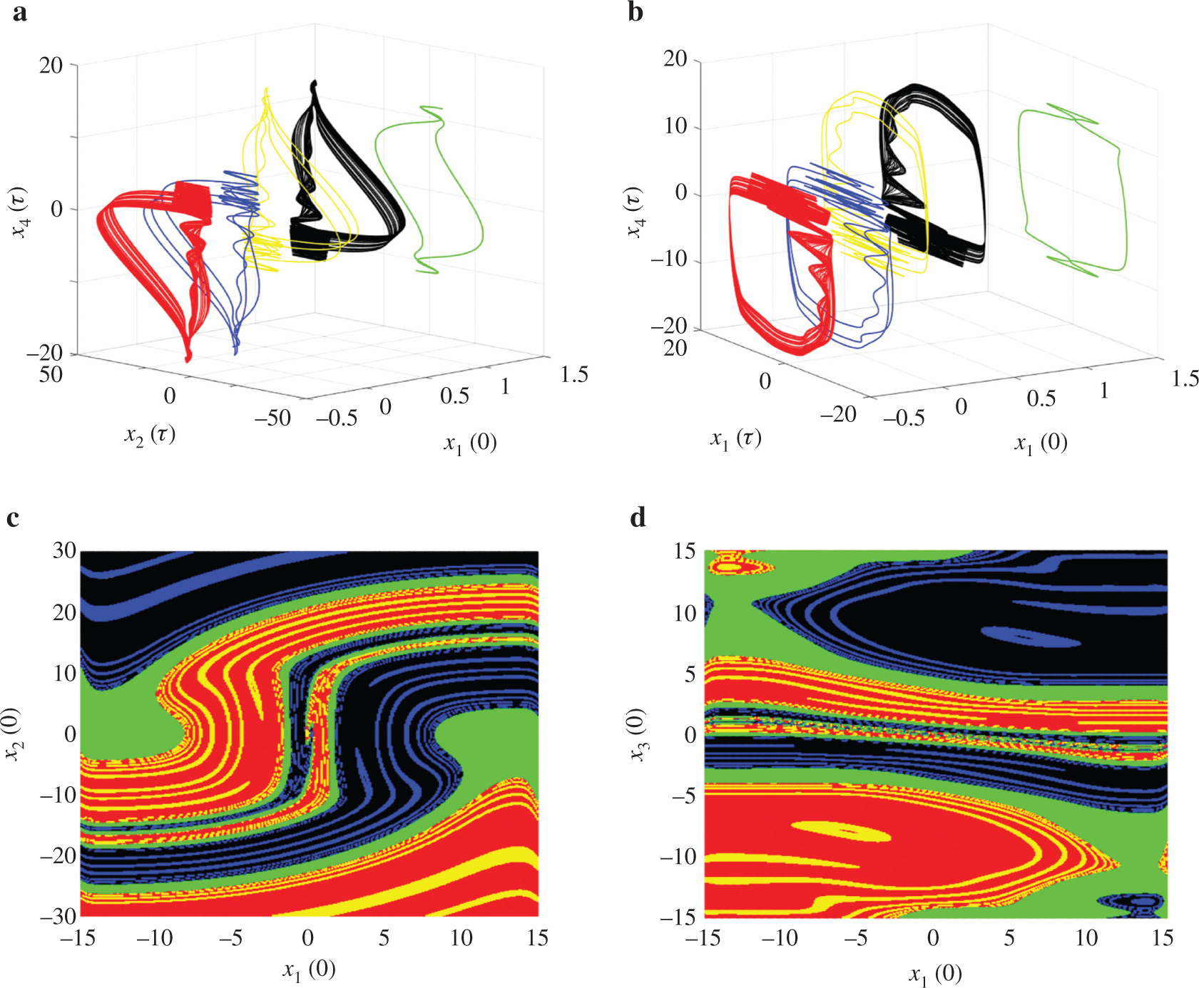
In the bifurcation diagram of Figure 6a, five sets of data (showing regions of hysteric dynamics and parallel bifurcation) obtained by varying upward the coupling strength μ are superimposed. Those in red and black (resp. green and yellow) colours are obtained by initialising integration from the initial state X(0) = (±0.1, 0, 0, 0, 0) (resp. X(0) = (±0.5, 0, 0, 0, 0)) while the one in blue is captured by integrating the system from the initial condition X(0) = (1.5, 0, 0, 0, 0). A very good coincidence can be noted between each bifurcation diagram and its corresponding maximum Lyapunov exponents in Figure 6b. From Figure 6, four regions/domains (i.e. I, II, III and IV) with three frontiers associated with a well-defined crisis are showing the transition from multistability to monostability in the controlled SHCCO. In region I (i.e. μ ∈ [0, 0.0864[), five disconnected attractors are coexisting (i.e. a pair of asymmetric period-3 cycle, a pair of asymmetric chaotic attractor and a symmetric period-1 attractor). This is clearly visible in the phase portraits of Figure 5a and their corresponding basin of attraction in Figure 5c,d for μ = 0. At the critical value μC1≈0.0864, the pair of asymmetric period-3 cycle disappear through an interior crisis. This is clearly confirmed by the brutal jump which is observed on the graph of the maximum Lyapunov exponent (in red colour) in Figure 6b. It is also worth mentioning that the crisis marks also the death of parallel branches which were associated with period-3 attractors; now, only hysteresis dynamic survives in the controlled system. Above the critical value μC1 of the coupling strength, starts region II (i.e. μ ∈ [0.0864, 0.4554[) where only three disconnected attractors now survive. These attractors are plotted in three-dimensional (3D) as depicted by the diagram of Figure 7a1 and the related basin of attraction in Figure 7a2 for μ = 0.25. One can notice that the pair of asymmetric chaotic attractors (red and black colours in Figure 7a) has survived the crisis and is coexisting with a symmetric quasi-periodic attractor (green colour in Fig. 7a). It is worth emphasising here that the pair of asymmetric chaotic attractors are associated with each branch of the bifurcation diagrams in the yellow and green coluors of Figure 6a. Indeed, after the interior crisis, the maximum Lyapunov exponent in red has jumped and its now quasi-perfectly superimposed with the one in green (see Fig. 6b) while their corresponding bifurcation diagrams are disconnected. That is to say, they have the same quantitative measure (Lyapunov’s exponent) but are qualitatively different (the size of the attractor in the state space). As the coupling strength is slightly increased, a boundary crisis is observed at the critical value μC2≈0.4554. That boundary crisis is characterised by the disappearance of one of the bifurcation diagrams (in blue) in Figure 6a which has jumped and is now perfectly superimposed with the bifurcation diagram in red (see region III of Fig. 6a). Clearly, that crisis has changed the system from a multistable state in region II with the coexistence of three disconnected attractors to bistable one in region III (i.e. 0.4554 < μ < 1.107). Now, the whole state space is covered by two asymmetric attractors as shown by the phase portraits and corresponding basin of attraction in Figure 7b (cyan and magenta colours). In region IV, former bistable attractors now collide with a unique symmetric attractor, thanks to another crisis (symmetry restoring crisis) at μC3≈1.107. The two routes which were existing in region III now collide at μC3 and only a unique symmetric attractor now survives in the controlled system (see see region IV in Fig. 6a). A phase portrait (resp. basin of initial conditions) of Figure 7c1 (resp. Fig. 7c2) is testifying to the effectiveness in the longterm of the linear control for higher values of the coupling strength. Also, with reference to Figure 7c1, when monostability is achieved in region IV, the surviving symmetric attractor has a substantially different structure than the one before the control has been applied (see phase portrait in green of Figs. 5a and 7c1, respectively).

Figure 7:

Some numerical phase portraits and corresponding cross section basin of attractions of the controlled system (4) captured for different values of coupling strength μ. (a) Three coexisting attractors [asymmetric pair of chaotic attractor (red and black colours) and symmetric quasi-periodic one (green colour)] when mu = 0.25; (b) two coexisting attractors in cyan and magenta colours when μ = 0.8; (c) Monostable periodic attractor (in green colour) when μ = 1.4. The rest of the system (4) parameters are: ε = 0.9873, σ = 0.3 and β = 0.7.

By following the same method as described Section 3 to obtain Figure 4a, we have plotted within the coexisting region of the control parameter ε (see Fig. 4a showing the coexistence of five disconnected attractors when the coupling strength μ = 0), several bifurcation diagrams of system (4) consider the different values of coupling strength μ. These figures show the transitions of different coexisting attractors when the coupling strength is increased. For each value of the coupling μ, three sets of data corresponding to increasing values of the bifurcation parameter ε starting from different initial conditions are superimposed (see Fig. 8). For μ = 0.25 (i.e. selected within region II of Fig. 6a), one can easily observe that three routes are still existing in the bifurcation parameter region ε (see Fig. 8a). These routes are linked to three coexisting attractors as the coupling strength μ is selected within region II of Figure 6a. Indeed, as on can see in Figure 8a, the two bifurcation branches in red and black colours are displaying the same dynamics but with different statistical properties. This last property is very helpful when tracking the magnetisation region of each coexisting attractor. When μ is fixed as 0.8 (i.e. selected within region III of Fig. 6a), only two periodic branches are now observed when varying ε (see Fig. 8b). The former bifurcation diagrams in the red and black colours of Figure 8a have collided to form a unique branch. This result is in accordance with the bistability obtained in Figure 7b. Finally, the monostability is confirmed in the coexisting region of control parameter ε when μ = 1.4 (selected within region IV of Fig. 6a). In fact, a unique periodic branch is observed in Figure 8c no matter the chosen initial condition during the numerical integration of the controlled system. This unique branch lead to the monostable periodic attractor presented in Figure 7c1.

Figure 8:

Bifurcation diagrams showing local maxima of state variable x₄ versus the control parameter α1∈[0.98,0.995] for different values of the coupling strength μ. Three sets of data are superimposed to show the effect the linear augmented controller on system (4). (a) μ = 0.25, (b) μ = 0.8 and (c) μ = 1.4.

6 Conclusion

In this paper, the complex dynamical behaviors of the SHCCO including hyperchaos and the coexistence of five disconnected attractors are first discussed. These results are confirmed through graphs of bifurcation diagrams, phase portraits, and diagrams of a two parameter map showing each dynamical behaviour which exists in the system. Both hysteresis and parallel bifurcation methods were used to uncover the coexistence of the five disconnected attractors (i.e. a pair of asymmetric chaotic attractors coexisting with a periodic symmetric one were obtained from hysteresis analysis while an asymmetric pair of period-3 was located through the parallel bifurcation method). Further, a linear augmentation strategy was implemented in another to drive the SHCCO from a multistable state to a monostable one. Numerical simulation results showed that for higher values of the coupling strength, the pair of asymmetric attractors which were coexisting with the symmetric periodic one were annihilated and only the symmetric one survives. The monostable attractor was achieved through three main crises namely, an interior crisis, a boundary crisis and a symmetry restoring crisis. After each crisis, the number of coexisting attractors decreased from five to three and then three to two and finally two to one. The obtained results on the control of multistability in the SHCCO in this work are more general than those presented in the literature [34], [35], [36], [37], [39] as we successfully controlled a system with five coexisting attractors. Indeed, to the best of the authors’ knowledge, the linear augmentation scheme has been applied so far only on systems with the coexistence of up to three disconnected attractors (with self-excited and hidden attractors).

It is worth emphasising that these results can be extended to other dynamical systems with self-excited or hidden attractors which have been reported so far.

References

[1] U. Feudel, Int. J. Bifurc. Chaos 18, 1607 (2008).10.1142/S0218127408021233Search in Google Scholar
[2] K. Ogata, Modern Control Eng. 2, 645 (1970).Search in Google Scholar
[3] F. T. Arecchi and F. Lisi, Phys. Rev. Lett. 49, 94 (1982).10.1103/PhysRevLett.49.94Search in Google Scholar
[4] F. T. Arecchi, R. Meucci, G. Puccioni, and J. Tredicce, Phys. Rev. Lett. 49, 1217 (1982).10.1103/PhysRevLett.49.1217Search in Google Scholar
[5] K. Sun and J. C. Sprott, Int. J. Bifurc. Chaos 19, 1357 (2009).10.1142/S0218127409023688Search in Google Scholar
[6] F. R. Tahir, S. Jafari, V.-T. Pham, C. Volos, and X. Wang, Int. J. Bifurc. Chaos 25, 1550056 (2015).10.1142/S021812741550056XSearch in Google Scholar
[7] V.-T. Pham, S. Vaidyanathan, C. Volos, S. Jafari, and S. T. Kingni, Optik-Int. J. Light Electron Optics 127, 3259 (2016).10.1016/j.ijleo.2015.12.048Search in Google Scholar
[8] S. Jafari, V.-T. Pham, and T. Kapitaniak, Int. J. Bifurc. Chaos 26, 1650031 (2016).10.1142/S0218127416500310Search in Google Scholar
[9] Q. Lai and L. Wang, Optik 127, 5400 (2016).10.1016/j.ijleo.2016.03.014Search in Google Scholar
[10] D. Dudkowski, S. Jafari, T. Kapitaniak, N. V. Kuznetsov, G. A. Leonov, et al., Phys. Rep. 637, 1 (2016).10.1016/j.physrep.2016.05.002Search in Google Scholar
[11] Z. T. Njitacke, J. Kengne, and A. Nguomkam Negou, Optik 130, 356 (2017).10.1016/j.ijleo.2016.10.101Search in Google Scholar
[12] Z. Wang, A. Akgul, V.-T. Pham, and S. Jafari, Nonlinear Dyn. 89, 1877 (2017).10.1007/s11071-017-3558-2Search in Google Scholar
[13] J. P. Singh and B. K. Roy, Optik 145, 209 (2017).10.1016/j.ijleo.2017.07.042Search in Google Scholar
[14] V. R. F. Signing, J. Kengne, and L. K. Kana, Chaos Soliton. Fract. 113, 263 (2018).10.1016/j.chaos.2018.06.008Search in Google Scholar
[15] F. Nazarimehr, K. Rajagopal, J. Kengne, S. Jafari, and V.-T. Pham, Chaos Soliton. Fract. 111, 108 (2018).10.1016/j.chaos.2018.04.009Search in Google Scholar
[16] B. Bao, H. Wu, L. Xu, M. Chen, and W. Hu, Int. J. Bifurc. Chaos 28, 1850019 (2018).10.1142/S0218127418500190Search in Google Scholar
[17] B. Bao, A. Hu, Q. Xu, H. Bao, H. Wu, et al., Nonlinear Dyn. 92, 1695 (2018).10.1007/s11071-018-4155-8Search in Google Scholar
[18] Q. Xu, Q. L. Zhang, H. Qian, H. G. Wu, and B. C. Bao, Int. J. Circ. Theor. Appl. 46, 1917 (2018).10.1002/cta.2492Search in Google Scholar
[19] T. F. Fonzin, K. Srinivasan, J. Kengne, and F. B. Pelap, AEU-Int. J. Electron. Commun. 90, 110 (2018).10.1016/j.aeue.2018.03.035Search in Google Scholar
[20] T. F. Fonzin, J. Kengne, and F. B. Pelap, Nonlinear Dyn. 93, 653 (2018).10.1007/s11071-018-4216-zSearch in Google Scholar
[21] S. Ren, S. Panahi, K. Rajagopal, A. Akgul, V.-T. Pham, et al., Zeitschrift für Naturforschung A 73, 239 (2018).10.1515/zna-2017-0409Search in Google Scholar
[22] J. C. Sprott, S. Jafari, A. J. M. Khalaf, and T. Kapitaniak, Eur. Phys. J. Special Topics 226, 1979 (2017).10.1140/epjst/e2017-70037-1Search in Google Scholar
[23] P. Prakash, K. Rajagopal, J. P. Singh, and B. K. Roy, AEU-Int. J. Electron. Commun. 92, 111 (2018).10.1016/j.aeue.2018.05.021Search in Google Scholar
[24] V.-T. Pham, C. Volos, and T. Kapitaniak, Systems with Hidden Attractors: From Theory to Realization in Circuits, Springer, Switzerland 2017.10.1007/978-3-319-53721-4Search in Google Scholar
[25] T. Baer, Josa B 3, 1175 (1986).10.1364/JOSAB.3.001175Search in Google Scholar
[26] C. C. Canavier, D. A. Baxter, J. W. Clark, and J. H. Byrne, Biol. Cybern. 80, 87 (1999).10.1007/s004220050507Search in Google Scholar
[27] A. N. Pisarchik and B. F. Kuntsevich, IEEE J. Quantum Electron. 38, 1594 (2002).10.1109/JQE.2002.805110Search in Google Scholar
[28] A. N. Pisarchik and U. Feudel, Phys. Rep. 540, 167 (2014).10.1016/j.physrep.2014.02.007Search in Google Scholar
[29] P. R. Sharma, M. D. Shrimali, A. Prasad, and U. Feudel, Phys. Lett. A 377, 2329 (2013).10.1016/j.physleta.2013.07.002Search in Google Scholar
[30] V. N. Chizhevsky and S. I. Turovets, Optics Commun. 102, 175 (1993).10.1016/0030-4018(93)90488-QSearch in Google Scholar
[31] A. N. Pisarchik and G. B. Krishna, Phys. Rev. Lett. 84, 1423 (2000).10.1103/PhysRevLett.84.1423Search in Google Scholar PubMed
[32] L. M. Pecora and T. L. Carroll, Phys. Rev. Lett. 67, 945 (1991).10.1103/PhysRevLett.67.945Search in Google Scholar PubMed
[33] C. Ainamon, S. T. Kingni, V. K. Tamba, J. B. C. Orou, and P. Woafo, J. Control Autom. 30, 501 (2019).10.1007/s40313-019-00463-0Search in Google Scholar
[34] P. R. Sharma, A. Sharma, M. D. Shrimali, and A. Prasad, Phys. Rev. E 83, 067201 (2011).10.1103/PhysRevE.83.067201Search in Google Scholar PubMed
[35] P. R. Sharma, A. Singh, A. Prasad, and M. D. Shrimali, Eur Phys. J. Special Topics 223, 1531 (2014).10.1140/epjst/e2014-02115-1Search in Google Scholar
[36] P. R. Sharma, M. D. Shrimali, A. Prasad, N. V. Kuznetsov, and G. A. Leonov, Eur. Phys. J. Special Topics 224, 1485 (2015).10.1140/epjst/e2015-02474-ySearch in Google Scholar
[37] P. R. Sharma, M. D. Shrimali, A. Prasad, N. V. Kuznetsov, and G. A. Leonov, Int. J. Bifurc. Chaos 25, 1550061 (2015).10.1142/S0218127415500613Search in Google Scholar
[38] K. Yadav, A. Prasad, and M. D. Shrimali, Phys. Lett. A 382, 2127 (2018).10.1016/j.physleta.2018.05.041Search in Google Scholar
[39] T. F. Fozin, R. Kengne, J. Kengne, K. Srinivasan, M. S. Tagueu, et al., Int. J. Bifurc. Chaos 29, 1950119 (2019).10.1142/S0218127419501190Search in Google Scholar
[40] K. Thamilmaran, M. Lakshmanan, and A. Venkatesan, Int. J. Bifurc. Chaos 14, 221 (2004).10.1142/S0218127404009119Search in Google Scholar
[41] M. Itoh, Int. J. Bifurc. Chaos 11, 605 (2001).10.1142/S0218127401002341Search in Google Scholar
[42] C. Li, W. Hu, J. C. Sprott, and X. Wang, Eur. Phys. J. Special Topics 224, 1493 (2015).10.1140/epjst/e2015-02475-xSearch in Google Scholar
[43] Z. T. Njitacke, J. Kengne, R. W. Tapche, and F. B. Pelap, Chaos Soliton. Frat. 107, 177 (2018).10.1016/j.chaos.2018.01.004Search in Google Scholar
[44] B. C. Bao, H. Bao, N. Wang, M. Chen, and Q. Xu, Chaos Soliton. Fract. 94, 102 (2017).10.1016/j.chaos.2016.11.016Search in Google Scholar
[45] B. A. Mezatio, M. T. Motchongom, B. R. W. Tekam, R. Kengne, R. Tchitnga, et al., Chaos Soliton. Fract. 120, 100 (2019).10.1016/j.chaos.2019.01.015Search in Google Scholar
[46] Z. T. Njitacke and J. Kengne, AEU – Int. J. Electron. Commun. 93, 242 (2018).10.1016/j.aeue.2018.06.025Search in Google Scholar
[47] G. D. Leutcho, J. Kengne, and L. K. Kengne, Chaos Soliton. Fract. 107, 67 (2018).10.1016/j.chaos.2017.12.008Search in Google Scholar
[48] R. L. M. Tagne, J. Kengne, and A. N. Negou, Int. J. Dyn. Control 7, 476 (2018).10.1007/s40435-018-0458-3Search in Google Scholar
[49] A. N. Negou, J. Kengne, and D. Tchiotsop, Chaos Soliton. Fract. 107, 275 (2018).10.1016/j.chaos.2018.01.011Search in Google Scholar
[50] A. Wolf, J. B. Swift, H. L. Swinney, and J. A. Vastano, Phys. D 16, 285 (1985).10.1016/0167-2789(85)90011-9Search in Google Scholar
[51] G. D. Leutcho and J. Kengne, Chaos Soliton. Fract. 113, 275 (2018).10.1016/j.chaos.2018.05.017Search in Google Scholar
[52] J. Kengne, S. M. Njikam, and V. R. F. Signing, Chaos Soliton. Fract. 106, 201 (2018).10.1016/j.chaos.2017.11.027Search in Google Scholar
[53] J. Kengne, Nonlinear Dyn. 87, 363 (2017).10.1007/s11071-016-3047-zSearch in Google Scholar
[54] J. H. Peng, E. J. Ding, M. Ding, and W. Yang, Phys. Rev. Lett. 76, 904 (1996).10.1103/PhysRevLett.76.904Search in Google Scholar PubMed
© 2020 Walter de Gruyter GmbH, Berlin/Boston
Articles in the same Issue
- Frontmatter
- Atomic, Molecular & Chemical Physics
- Selection of Single Harmonic Emission Peak for Producing Isolated Attosecond Pulse via Chirped-UV Combined Field
- Dynamical Systems & Nonlinear Phenomena