An Investigation of the Forced Convection and Heat Transfer with a Cylindrical Agitator Subjected to Non-Newtonian Nanofluids
-
Botong Li
 ,
Liancun Zheng
,
Liancun Zheng

Abstract
The present research performed a numerical simulation of laminar forced convection nanofluid-based non-Newtonian flow in a channel connecting a tank with heating regions. To achieve a rapid diffusion of heat, a cylindrical agitator is inserted into the tank. Power-law modelling is employed to describe the effect of non-Newtonian behaviour. The velocity and temperature fields and heat transfer coefficient ratio are studied systematically, taking into account the impact of various parameters, such as the generalised Reynolds number Re, generalised Prandtl number Pr, angular velocity of a cylinder ω, nanoparticle volume fraction ϕ, mixer size and location. Our research reveals that, to improve the heat transfer in practice, several applicable strategies are available, including the addition of more nanoparticles into the base fluid, which proved to be the most efficient method to enhance the heat transfer of a nanofluid.
1 Introduction
Thermal management is vital for many devices used in engineering, such as the frequency convertors, power supplies, and amplifiers [1]. In heat exchangers, nanosized particles with different sizes and shapes are often added into the base fluid of cooling liquids to obtain better heat transfer with less pressure drop [2]. Ever since Choi and Eastman [3] first suspended small particles (average particle size less than 100 nm) in fluids, which was already proven to enhance the thermal performance of pure fluids, this nanofluid was adopted in various kinds of industrial equipments, as summarised in [4], [5]. Kamyar et al. [6] listed some important literature details about the computational fluid dynamics (CFD) of nanofluids in the applications. Eid [7] analysed the mixed convective of a magnetohydrodynamic nanofluid flowing through a porous medium. The boundary layer on the exponentially stretching sheet with the chemical interaction and the heat generation/absorption effects was focussed.
In this research, one special kind of nanofluids, i.e. the non-Newtonian nanofluid is focussed on. This type of nanofluid can be obtained by two strategies: a nanofluid whose base fluid is Newtonian flow and that shows non-Newtonian behaviour [8], and a non-Newtonian base fluid which does not alter its former rheological behaviour when nanoparticles are suspended in it. The flow and heat transfer of non-Newtonian fluids play a pivotal part in many industrial processes such as glass blowing, biological solutions such as blood, and the extrusion of polymeric melts and fluids. Some researchers also point out that they can be employed as useful cooling enhancing mediums in electronic modules and heat exchangers [9].
Furthermore, investigations on the fluid flow and heat transfer behaviours of non-Newtonian nanofluids applied in various industrial processes are important. Some critical studies on non-Newtonian nanofluids were included but were not limited to the following. Santra et al. completed a study on the heat transfer of non-Newtonian type nanofluids in a two-dimensional horizontal rectangular duct with infinite depth [10]. Eid and Mahny [11] focussed on the steady flow and heat transfer of a Sisko nanofluid in a porous medium and they considered a nonlinearly stretching sheet in the existence of heat generation/absorption. Ellahi et al. [12], [13], [14] employed the Vogel’s model and the Reynolds’ model to investigate the non-Newtonian nanofluids. Eid et al. [15] used the two-phase flow model for a generalised non-Newtonian Carreau nanofluid under the influence of magnetic fields and thermal radiation, and a permeable nonlinearly stretching surface was considered in the existence of suction/injection. Esmaeil Nejad et al. [16] studied numerically the convection flow and heat transfer of power-law nanofluids in a rectangular micro-channel by adopting the two-phase mixture model. Hatami and Ganji [17] performed heat transfer analysis of a non-Newtonian nanofluid located between two coaxial cylinders both numerically and analytically. It was noted that sodium alginate was the base non-Newtonian fluid and TiO2 nanoparticles were suspended in it. Eid and Mahny [18] addressed the unsteady boundary layer convective problem of the heat and mass transfer of a non-Newtonian nanofluid in a magnetic field with heat generation or absorption.
Special attention should be paid to the fact that a new type non-Newtonian fluid is formed when nanoparticles are suspended in a non-Newtonian fluid, as explained in [19]. Thus, the rheology of non-Newtonian nanofluids can be changed by the addition of some volume fraction of nanoparticles. Eshgarf and Afrand [20] studied the rheological behaviour of a non-Newtonian fluid, i.e. COOH functionalised MWCNTs-SiO2/EG-water hybrid nanocoolant, and they found that the consistency index and power law index of nanofluids were varying with temperature and the solid volume fraction from 27.5 °C to 50 °C. Santra et al. [10] employed two empirical constants m and n, which are borrowed from [21], to depict the rheological characteristics of a non-Newtonian nanofluid working as a cooling medium. In our work, it is also assumed that the rheological characteristics of non-Newtonian nanofluids are not unchanged with different amount of nanoparticles adding in it. The power-law index n and the consistency coefficient m are regarded as changeable with the particle loading parameter ϕ, as in Hojjat et al.’s experiments with water-carboxy methyl cellulose (CMC)/TiO2 nanofluid [22]. This changeable assumption promises accurate predictions for fluid flow and heat transfer of nanofluids in precise equipment designs. For nanofluids, the commonly used nanoparticles include metal oxides, oxide ceramics [23] and chemically stable metals (e.g. copper), one among many of which are very expensive. In this work, a relatively cheap and widely applied nanoparticle, i.e. TiO2 is chosen. TiO2 has a wide range of applications: sunscreen, printing inks, rubber, cosmetic products, food colouring, etc., among which the most important applications are paints, varnishes, paper, and plastics. Abdolbaqi et al. [24] presented an experimental investigation on the bioglycol/water-based TiO2 nanofluids and they measured the heat transfer coefficient and friction factor under a turbulent flow condition. Chen and Cheng [25] adopted CFD to simulate the steady incompressible forced convective turbulent fluid flow and heat transfer of a TiO2/water nanofluid in three-dimension. Eid [26] analysed the behaviours of the nanofluid for three different nanoparticles in a H2O-base fluid, namely, (Cu-NPs), (Al2O3-NPs) and (TiO2-NPs), while considering the influence of the chemical reaction.
Inspired by the above works, a channel connecting a tank with a continuous stirrer is our configuration of interest, which has vital engineering applications. This configuration can be adopted to simulate flow around air foils, buildings, and power system collectors [27], but our research will focus on another application. This type of channel and tank can be used in food and drug engineering for stirring nanofluids. As it is well known, nanofluids used in modern industry are always pre-treated by mixing. For example, food and nanodrugs are mixed in a microchannel for better controllable delivery and fast heat diffusion [19]. In such up-to-date applications, a fast and thorough mixing of the fluid is often required. Hence, active mechanical stirring is needed instead of the primary and slow diffusion mechanism of the fluid. Islami et al. [19] studied the problem of a two-dimensional non-Newtonian nanofluid in a microchannel when micromixers are employed or not for varying nanoparticle volume fractions and varying Reynolds numbers (Re). Alam and Kim [28] numerically investigated on how to mix fluids in a microchannel when its side walls have grooves and three-dimensional Navier-Stokes equations were solved. In this investigation, to achieve rapid heat diffusion, a cylindrical agitator is inserted into the tank to enhance the advection result via stretching, splitting, folding and breaking liquid flows. This work will analyse the laminar non-Newtonian nanofluids when forced convection happens with heating boundary conditions. The finite element method (FEM) with modified techniques was adopted. The results and figures revealing the influences of the generalised Reynolds number Re, generalised Prandtl number Pr, angular velocity of cylinder ω, nanoparticle volume fraction ϕ, mixer size and location on the heat transfer and velocity field are compared and provided.
2 Description
2.1 Definition of Geometry
The configuration of the physical problem investigated in this paper is demonstrated in Figure 1. A channel connecting a tank with a continuous stirrer is considered, and so the flow field widens suddenly. The width of the channel is L, while the width of the tank is 3L. Note that the channel should be long enough such that the fluid flow is fully developed. Uniform temperature is imposed at the inlet of the channel, while wall heaters are arranged symmetrically. Other parts are adiabatic. An adiabatic rotating cycloidal mixer with a diameter of L is placed at the exit of the channel where the origin point of the coordinate system is placed at the centre of the cycloidal mixer. In our investigation, the cylinder position and its size will be changed, when the effects of the angular velocity of the mixer, the nanoparticle volume fraction, base-fluid characteristics, the Re and Pr on the velocity and temperature fields are revealed.
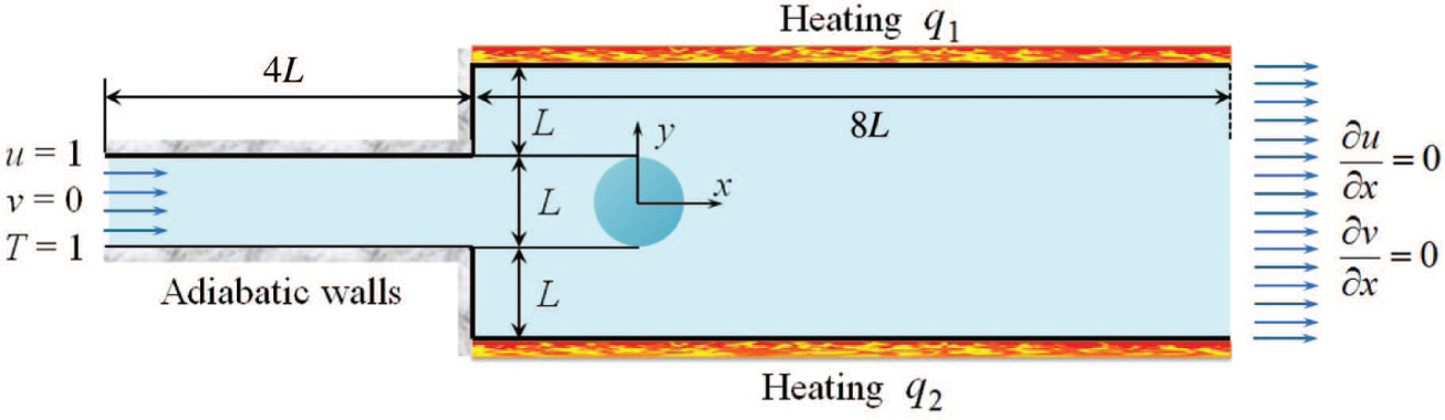
The nanofluid flowing through the channel into the tank with heating regions.
2.2 Governing Equations
Consider laminar and the forced convection nanofluids in the channel and the tank. A similar geometrical domain was studied previously [29], [30]. Assuming the nanofluid acts as a single-phase fluid in a steady state of two-dimension and thermal equilibrium. No chemical interaction happens; and the nanofluid employed in this research is of the pseudoplastic type and the power-law model is adopted for modelling the apparent viscosity.
The governing equations are:
Continuity:
Momentum [31]:
where ρnf is the nanofluid density; u = (u, v) is the velocity, where u presents the horizontal component and v the vertical one; p represents the hydrostatic pressure; and μnf denotes the consistency index of the nanofluid. In the power-law model, the formula of σu is
where n is the power-law index.
Energy [32]:
where the subscript nf refers to the nanofluid, cp is the specific heat, and T denotes the temperature. The parameter knf is the effective thermal conductivity. Additionally, assuming a uniform nanofluid, concentration equations will not be involved [33].
2.3 Thermophysical and Rheological Properties
By using the classical single phase mixture assumption, the effective density of the nanofluid is defined as [27]:
Furthermore, by employing the thermal equilibrium conditions, the nanofluid specific heat is given as [9], [34]:
where the particle loading parameter is ϕ, and subscripts p and bf represent the particle and the base fluid, respectively.
The current investigation evaluates the fluid flow and heat transfer of a power-law nanofluid containing TiO2 nanoparticles. An aqueous solution of CMC whose concentration is 0.5 wt% as the power-law typed base fluid is chosen. The aqueous CMC solution is a pseudoplastic fluid. According to the experimental study of literature [35], the physical properties of a CMC-water (<0.4 %) solution is very similar to water, which is given in Table 1.
The physical properties of the base fluid of CMC-water and nanoparticles.
| Property | TiO2 | CMC-water |
|---|---|---|
| ρ (kg/m3) | 4250 | 997.1 |
| cp (J/kg ⋅ K) | 686.2 | 4179 |
| Particle size (nm) | 10 [25] |
The consistency index, power law index and thermal conductivity measured by Hojjat et al. and Eid in their experiments [22], [36] for a water-CMC/TiO2 nanofluid with varying concentrations will be employed (see Tab. 2). This paper will only address non-Newtonian power-law nanofluids, with parameters that meet these restrictions.
2.4 Nondimensionalisation and Boundary Conditions
To nondimensionalise (1)–(4), x and y are scaled by L; u and v are scaled by U0; the pressure p is scaled by
where
Additionally,
A system of nondimensional boundary conditions is employed (also see Fig. 1):
At the inlet: u = 1, v = 0, T = 1;
At the heating walls of the tank, downstream of the channel (defining the left side of the direction of the flow as the left wall and defining the right side in a similar way):
At the outlet:
On the other walls:
On the cylinder’s surface:
where qi is the heat flux for each heater, and ω denotes the cylinder angular velocity. In the following section, (x0, y0) = (0, 0) unless the location of the mixer is investigated specifically.
3 Numerical Scheme
3.1 Weak Formulation
The FEM with the aid of Freefem
The domain is defined as Ω ⊂ R2, and the boundary of Ω is Γ, which is sufficiently smooth (e.g. Lipschitz continuous). The velocity u and v is considered in space Z, defined as H1(Ω) if n ≤ 1 or
where ε is set to be ε = 10−6 in the following computations. The weak formulations of (8) and (9) are:
where
It should be noted that the weak formulation (12) contains the term
3.2 Iterative Finite Element Scheme
The domain will be triangulated into a nonuniform triangular mesh. A representative triangular mesh is shown in Figure 2.
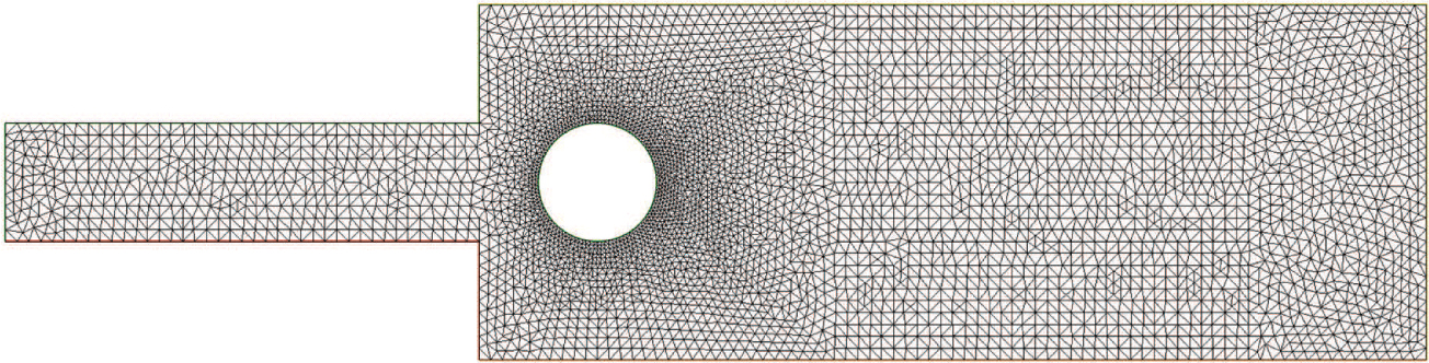
A representative triangular mesh with 8668 grids in the calculated domain.
Continuous finite elements are used. Quadratic polynomial approximations in every element are employed for u, v and T, and a linear approximation is adopted for p. To handle the nonlinear terms σu and σ0, an iterative method is introduced into (11–12), i.e. the so-called ‘ghost’ time. dt > 0 is the time step size.
where
The total time step can be regarded as the number of iterations. The continuity equations and the momentum equations are independent of the temperature equation. Therefore, they can be first solved to obtain only the velocity and the pressure. By substituting both the velocity and the pressure into the temperature equation, the temperatures can be obtained. The iterative process stops as soon as the steady state is obtained, and the velocity stops changing. The iterative solutions will definitely be an approximation of the steady-state equation solutions.
To validate the iterative process, its velocity results are compared with those obtained by analytical results [37] in the case of laminar non-Newtonian power-law fluids in semi-infinite parallel plate channel. From Figure 3, it can be found out that these results agree well (i.e. the maximal deviation is 5.1 %).

Comparison of velocities between results obtained by present method and former analytical technique when the physical characteristics of the fluid are n = 1.2, Re = 50.
For further validation, the present numerical method was adopted to calculate the velocity of similar work found in other literature. Selimefendigil and Öztop [27] investigated the mixed convection of nanofluid in a channel with a backward facing step, which also has a rotating cylinder like ours inserted into it. The results obtained by the numerical method in the present research are compared with the solutions obtained by those researchers in Figure 4. A special case when
![Figure 4: Results obtained by the method in present work in comparison with those from other literature [27].](/document/doi/10.1515/zna-2018-0013/asset/graphic/j_zna-2018-0013_fig_004.jpg)
Results obtained by the method in present work in comparison with those from other literature [27].
3.3 Grid Independence and Time Consumption
In the following section, the grid independence and time consumption comparisons with varying mesh densities are executed to find an optimal mesh with preferable results and a relative minimal computational time.
To reveal the impact of calculation of meshing, four different grid sizes are compared and the temperatures along the right wall of the tank are checked in Figure 5. The results at ω = 1.0, Re = 100, Pr = 2.0, ϕ = 4 %, q1 = q2 = −1 are revealed. It is worth mentioning that the grid size in Figure 5 is the total number of grids in the channel and the tank. From this figure, it can be seen that differences only occur between −1 and 0, and the grid size of 8668 is chosen to resolve the flow and thermal fields in our later computation. Additionally, Figure 5 shows the running time for the computation when a personal laptop possessing an Intel(R) Core(TM) which has an i7-3520 M CPU working at 2.90 GHz and a 4.00 GB RAM is used.
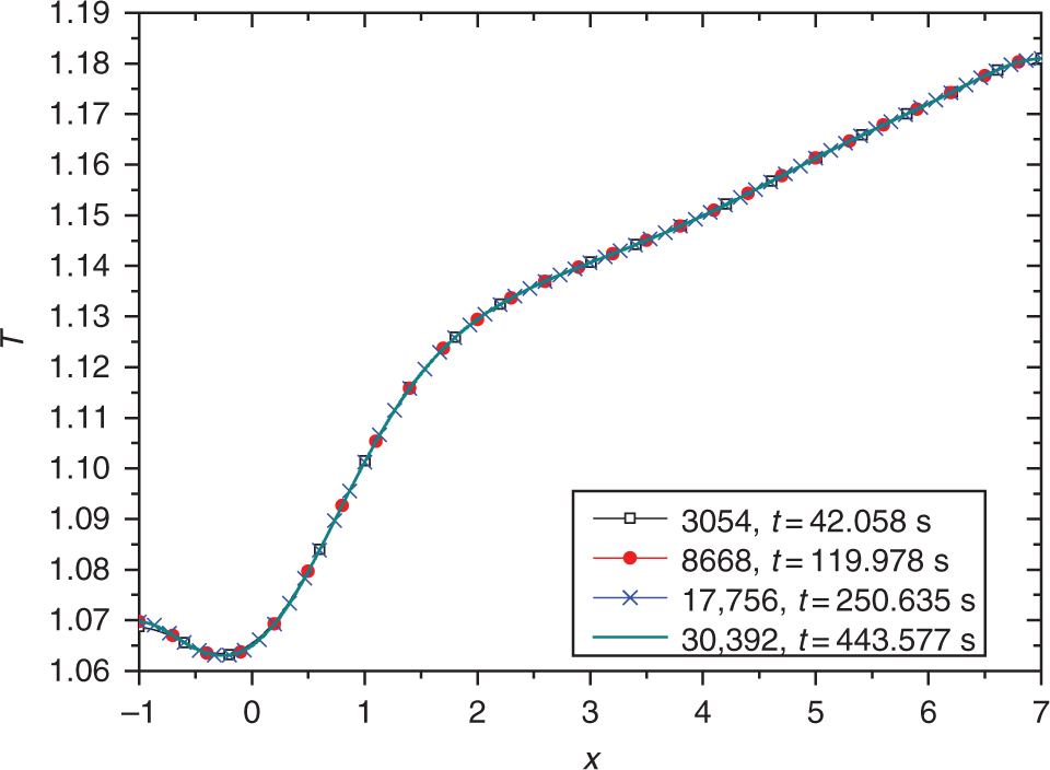
Impact of the grid density on temperatures at the right wall of the tank.
4 Results and Discussion
This section primarily presents the velocity field, temperature field, and heat transfer calculated from FEM for different sets of parameters such as the generalised Pr, generalised Re, ω, and ϕ. The compared results are in a dimensionless form, and the ranges of the parameters are: 100 ≤ Re ≤ 500, 0.5 ≤ Pr ≤ 4, −4 ≤ ω ≤ 4, 0 ≤ ϕ ≤ 4 %.
In this research, the definition of the generalised is
The consistency index, the power law index and the thermal conductivity of the nanofluid [22], [36].
| ϕ (%) | μ | n | k (W/m⋅K) |
|---|---|---|---|
| 0 | 0.145 | 0.542 | 0.600 |
| 1 | 0.190 | 0.526 | 0.603 |
| 3 | 0.240 | 0.502 | 0.641 |
| 4 | 0.365 | 0.485 | 0.740 |
4.1 Generalised Reynolds Number
Flow patterns of interest are shown in Figure 6 through the depiction of velocity profiles perpendicular to the tank walls located at x = −0.5 (just upstream of the mixer) and x = 1 (just downstream of the mixer) for various generalised Re. It is found that the amplitude of the fluctuation of the u-velocity curve becomes greater as the generalised Re rises for the enhanced kinetic energy. In Figure 6a, the values of u-velocity reach negative values for the recirculation cells that exist in the zone that locate both upstream of the mixer and downstream of the channel.
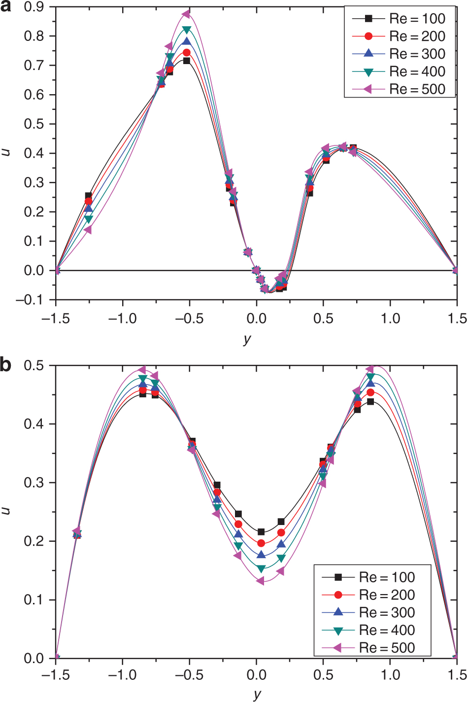
u-Velocity profiles perpendicular to the tank walls for different generalised Re when ω = 1, Pr = 2.0, ϕ = 4 %, q1 = q2 = −1 at (a) x = −0.5; (b) x = 1.
Figure 7 depicts the temperature profiles both perpendicular to the tank walls and along the tank walls. It is worth mentioning that as the generalised Re increases, the differences between temperatures in the left part of the fluidic area and the right part decrease. The temperature near the right wall should be completely different from those near the left wall for the inserted rotating cylinder. However, when the generalised Re increases, the fluid is flowing faster and the heat exchange between liquid molecules becomes frequent and violent, which, to a certain extent, weakens the effects of the redistribution of heat and the uneven temperature field caused by agitation.
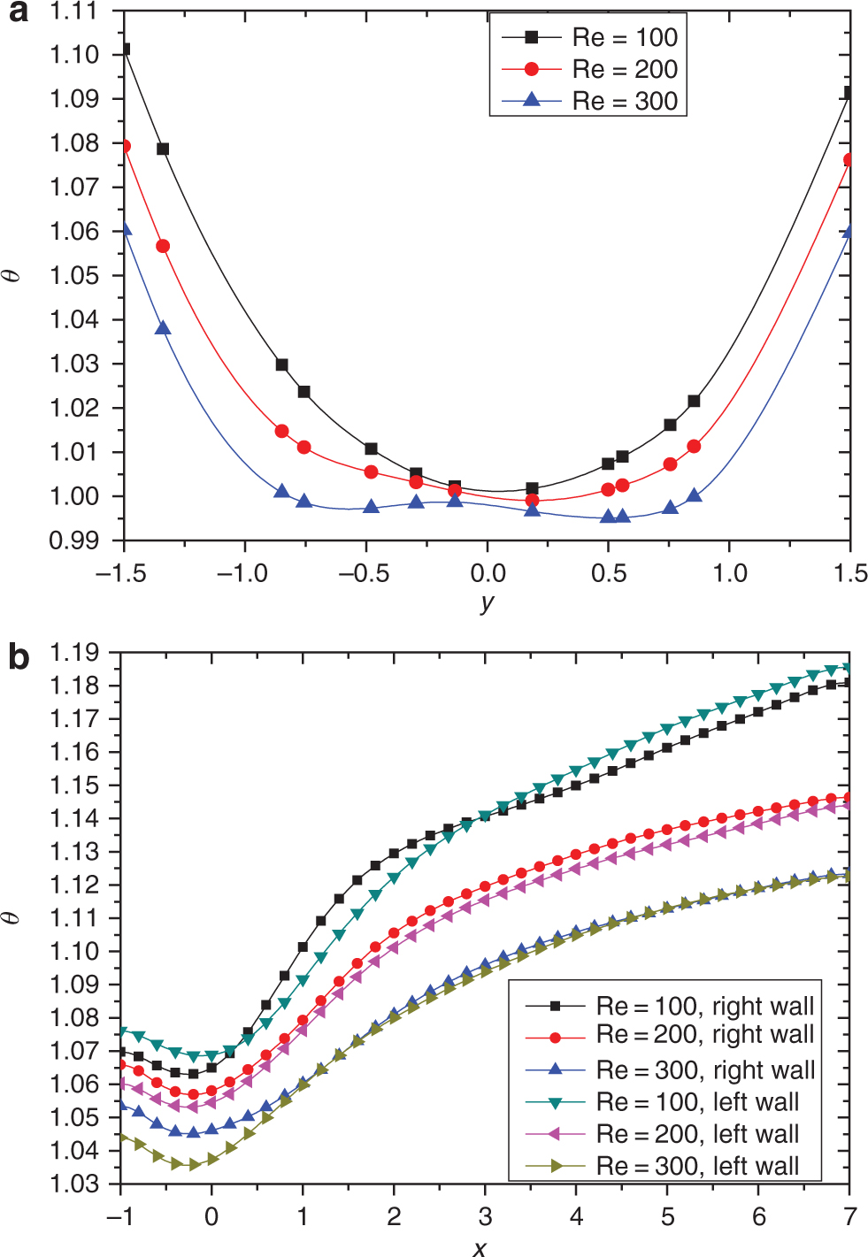
Temperature profiles at (a) x = 1 perpendicular to the tank walls; (b) along the tank walls for different generalised Re when ω = 1, Pr = 2.0, ϕ = 4 %, q1 = q2 = −1.
4.2 Generalised Prandtl Number
The influence of the generalised Pr on the temperature field is shown in Figures 8 and 9. In Figure 8, the difference between temperatures on the left wall and on the right wall is obvious when Pr = 0.5. As the generalised Pr increases, the difference becomes less evident. This is simply because a larger Pr means a smaller thermal conductivity, which weakens the effect of the heat transfer and the temperature differences decrease. In addition, the isotherms in Figure 9 present a brief comparison for varying the generalised Pr at a fixed value of ω = 1, Re = 100, ϕ = 4 %, q1 = q2 = −1.
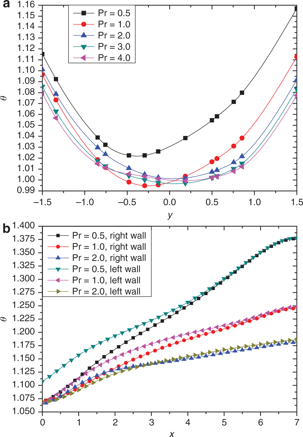
Temperature profiles at (a) x = 1 perpendicular to the tank walls; (b) along the tank walls for different generalised Pr when ω = 1, Re = 100, ϕ = 4 %, q1 = q2 = −1.
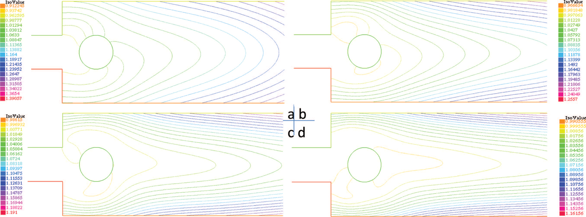
Isotherms for different generalised Pr when ω = 1, Re = 100, ϕ = 4 %, q1 = q2 = −1: (a) Pr = 0.5; (b) Pr = 1.0; (c) Pr = 2.0; (d) Pr = 3.0.
4.3 Angular Velocity of Mixer
The Re and the Pr play a key role when the fluid flow and heat transfer in the channel and the tank are investigated. However, sometimes, these dimensionless parameters are hard to change. In the following sections, the effects of the rotation rate, the nanoparticle volume fraction, and the geometry size and location of the mixer on the velocity and temperature fields are studied.
Velocity and temperature profiles perpendicular to the tank walls at x = 1 for different angular velocities are shown in Figure 10. It seems that both the velocity and the temperature curves are very sensitive to the angular rotational speed of the mixer. The presence of a recirculation cell located downstream of the mixer can be observed, indicated by the fact that the curve of the u-velocity possesses a trough of wave. Additionally, it is noticeable that the curves for clockwise rotation and the curves for counter-clockwise rotation are symmetrical about y = 0 for both the velocity and the temperature.
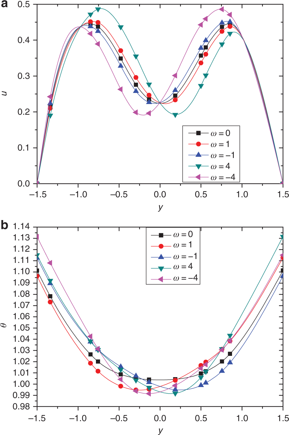
(a) Velocity profiles and (b) temperature profiles at x = 1 perpendicular to the tank walls when Pr = 1.0, Re = 100, ϕ = 4 %, q1 = q2 = −1 for various angular velocities.
Figure 11 demonstrates the temperature of both the left and the right wall of the tank with Pr = 1.0, Re = 100, ϕ = 4 % , q1 = q2 = −1 for different angular velocities. When the angular velocity ω is zero, the temperatures of both sides of the tank walls are equal. At the same angular velocities, the temperature of the left side of the tank wall with a clockwise rotating mixer is equal to the temperature of the right side wall with a counter-clockwise rotating mixer. The most important phenomenon is that increasing the angular velocity of the rotating mixer will definitely increase the temperatures of the walls due to the mixer speeding up the heat transfer of the fluid field.

Temperature profiles along the tank walls for different angular velocities when Pr = 1.0, Re = 100, ϕ = 4 %, q1 = q2 = −1.
4.4 Nanoparticle Volume Fraction
The impacts of the nanoparticle volume fraction ϕ on the temperatures at the upstream edge x = −0.5 and downstream edge x = 0.5 of the rotating mixer for Pr = 1.0, Re = 100, ω = 3, q1 = q2 = −1 are shown in Figure 12. The temperature profiles are definitely asymmetrical for the rotating mixer. From the figure, it obviously shows that the nanofluid heating effect is less protruding as the particle loading parameter ϕ increases. The decrease in temperature with a higher nanoparticle volume fraction is caused by a combination effect of a decreasing power-law index n, an increasing consistency index μ and an increasing thermal conductivity k. As it can be seen from Table 2, when the nanoparticle volume fraction increases, the power-law index n will decrease while the consistency index μ and the thermal conductivity k will increase. The temperature changes with the three quantities n, μ, and k. With a lower power-law index n, and a higher thermal conductivity k, the temperature will decrease, but with a higher consistency index μ, the temperature will increase. In Figure 12, the temperature decreases when all the three parameters are varying, because the power-law index n and the thermal conductivity k play a more prominent part in the nanofluid heating effect. From a physical point of view, lowering the power-law index n will shear-thin the fluid, which increases the velocity. As a result, the higher velocity will act on the temperature equation, and reduce the temperature. In addition, the thermal conductivity reflects the heat transfer ability of the fluid, which dominates the temperature change.

Temperature profiles perpendicular to the tank walls when Pr = 1.0, Re = 100, ω = 3, q1 = q2 = −1 for different nanoparticle volume fraction at (a) x = −0.5; (b) x = 0.5.
Figure 13 shows the effects of the nanoparticle volume fraction on the temperature fields for constant parameters of Pr = 1.0, Re = 100, ω = 3, q1 = q2 = −1. The shapes of the temperature curves broadly do not change with a varying nanoparticle volume fraction, but the strength changes. Obviously, the employment of nanoparticles alters the magnitude of the heating impacts on the temperatures on the walls. Additionally, the temperatures on the left wall are higher than the ones on the right walls due to the presence of the rotating mixer.

Temperature profiles along the tank walls for different nanoparticle volume fraction when Pr = 1.0, Re = 100, ω = 3, q1 = q2 = −1.
In the present research, all of the variables are calculated in their dimensionless forms. In Figure 14, an increased loading of nanoparticles suspended in the base fluids causes a rising pressure for the increased viscosity. It also reveals the curve of the pressure drop turn at the position of the stirrer, so it is clearly possible to determine the location of the agitator using the curve. Big pressure drops are always regarded as unfavourable effects. Thus, when nanofluids are used in the stirring tank, the particle loading parameter should be carefully selected because the pressure drop must be controlled to be in a certain range.
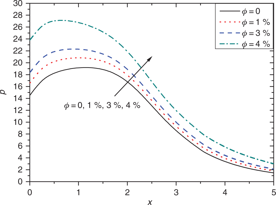
Influence of the particle loading parameter ϕ on pressure when Pr = 1.0, Re = 100, ω = 3, q1 = q2 = −1.
The horizontal velocity profiles for dimensionless Pr = 1.0, Re = 100, ω = 3, q1 = q2 = −1 and various values of ϕ are depicted in Table 3. At both x = −0.5 and x = 0.5, the velocity fields are fully developed through the channel into the tank, so this table can clearly present the influence of ϕ on the velocity profiles. The velocity increases a small amount as the particle volume fraction increases. As the particle volume fraction rises, the pseudoplasticity effect of the fluid becomes strong (refer to Tab. 2), which in turn indicates a higher speed of the fluid velocity. However, it can also be determined from Table 2 that, as the particle volume fraction increases, the consistency index of the fluid gets bigger, which reduces the values of the velocity. These two effects interact with each other, and the velocity ultimately increases a small amount.
Velocity profiles perpendicular to the tank walls when Pr = 1.0, Re = 100, ω = 3, q1 = q2 = −1 for various nanoparticle volume fractions at x = −0.5 and x = 0.5.
| x = 0.5 | x = −0.5 | ||||||||
|---|---|---|---|---|---|---|---|---|---|
| y | u | y | u | ||||||
| ϕ = 0 | ϕ = 1 % | ϕ = 3 % | ϕ = 4 % | ϕ = 0 | ϕ = 1 % | ϕ = 3 % | ϕ = 4 % | ||
| −1.5 | 0 | 0 | 0 | 0 | −1.5 | 0 | 0 | 0 | 0 |
| −1.33833 | 0.22034 | 0.22013 | 0.21993 | 0.21937 | −1.29 | 0.03234 | 0.03192 | 0.03151 | 0.03038 |
| −0.82125 | 0.49615 | 0.49619 | 0.49614 | 0.49622 | −1.20909 | 0.05119 | 0.05076 | 0.05033 | 0.04918 |
| −0.69098 | 0.50387 | 0.50402 | 0.50408 | 0.50444 | −1 | 0.09667 | 0.09649 | 0.09634 | 0.09588 |
| −0.29675 | 0.40898 | 0.40969 | 0.41035 | 0.41223 | −0.74128 | 0.21284 | 0.21308 | 0.21334 | 0.214 |
| −0.12308 | 0.33772 | 0.33837 | 0.339 | 0.34074 | −0.65086 | 0.28418 | 0.28449 | 0.28483 | 0.28568 |
| 0.08241 | 0.27303 | 0.27353 | 0.27404 | 0.27538 | −0.48566 | 0.46531 | 0.4656 | 0.46589 | 0.46666 |
| 0.14675 | 0.26062 | 0.26108 | 0.26155 | 0.26277 | −0.24836 | 0.75044 | 0.75056 | 0.75066 | 0.75098 |
| 0.29219 | 0.25753 | 0.25788 | 0.25827 | 0.25923 | 0.26993 | 0.70332 | 0.70347 | 0.70361 | 0.70401 |
| 0.38813 | 0.26131 | 0.26158 | 0.26189 | 0.26262 | 0.81691 | 0.15102 | 0.15109 | 0.15117 | 0.15136 |
| 0.43751 | 0.27441 | 0.27461 | 0.27486 | 0.2754 | 0.90721 | 0.11097 | 0.11094 | 0.11094 | 0.11087 |
| 0.53281 | 0.28691 | 0.28697 | 0.28708 | 0.28724 | 1 | 0.08135 | 0.08122 | 0.08111 | 0.08076 |
| 0.64615 | 0.30119 | 0.30101 | 0.3009 | 0.30045 | 1.08462 | 0.05836 | 0.05814 | 0.05793 | 0.05735 |
| 0.74582 | 0.3123 | 0.31187 | 0.31148 | 0.31032 | 1.20909 | 0.04148 | 0.04115 | 0.04083 | 0.03996 |
| 0.85432 | 0.31681 | 0.31612 | 0.31548 | 0.31367 | 1.29 | 0.02582 | 0.02549 | 0.02517 | 0.02432 |
| 1.5 | 0 | 0 | 0 | 0 | 1.5 | 0 | 0 | 0 | 0 |
4.5 Mixer Size and Location
In the above section, the diameter of the mixer is kept at 1.0 and the distance from the centre of the mixer to the exit of the channel is also kept at 1.0 in dimensionless form. However, the mixer size and location play a very important role when the velocity and the temperature fields of the tank are calculated, as shown in the following.
Figure 15 reveals the effect of the size of the mixer on the temperature profiles on the walls. An interesting phenomenon is observed: the temperatures of the walls rise greatly with a bigger mixer. For example, at x = −1, the temperature rises 3.9 % from d = 1.0 to d = 1.5 on the left wall, and at x = 7, the temperature rises 3.4 % from d = 1.0 to d = 1.5 on the right wall. It looks like the temperature fields could be adjusted by changing only the size of the mixer: the bigger the mixer, the higher the temperatures. From a physical point of view, it can be easily explained. With a bigger mixer, much more fluid is disturbed. The heat enhancement occurs as a consequence of more liquid molecules moving and interacting with each other.
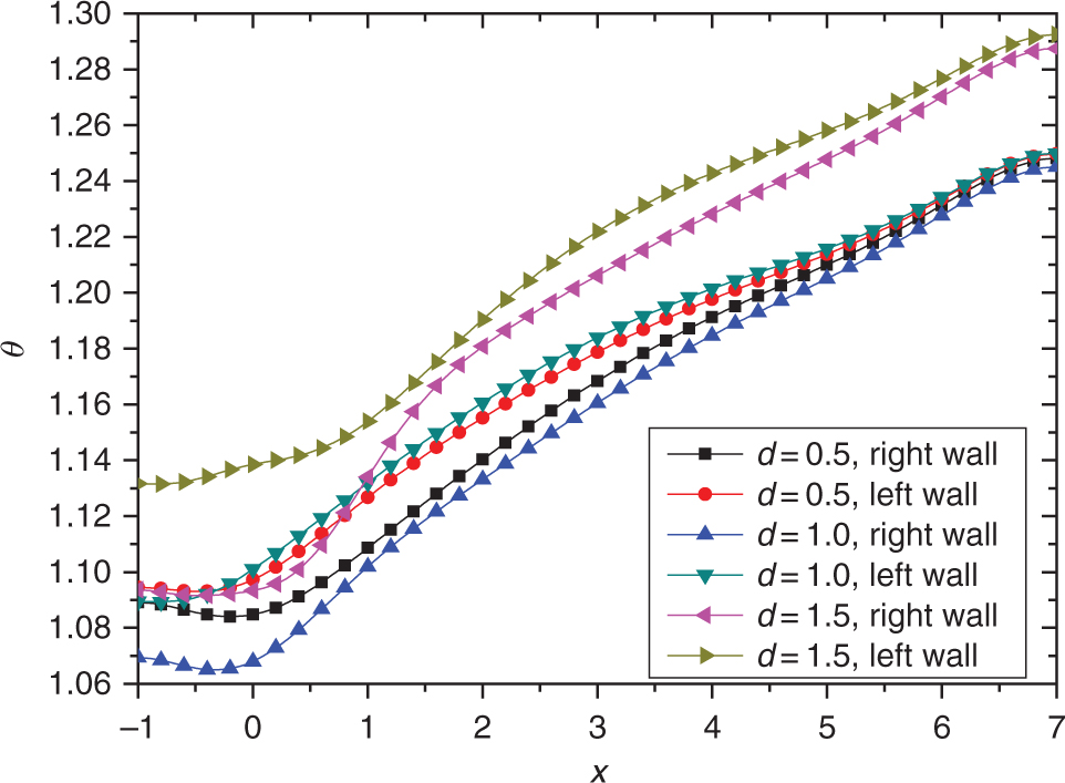
Temperature profiles along the tank walls for different mixer diameters when Pr = 1.0, Re = 100, ω = 3, q1 = q2 = −1, ϕ = 4 %.
The beautiful symmetrical patterns in Figure 16 shows the u-velocity for different mixer locations when Pr = 1.0, Re = 100, ω = 3, q1 = q2 = −1, ϕ = 4 %, d = 1. The parameter Z presents the distance from the centre of the mixer to the exit of the channel. The u-velocities with y = −0.5 and y = 0.5 parallel to the tank walls are just along the edges of the mixer. It looks like the u-velocity profile will translate as the location of the mixer moves. For a single velocity curve, it fluctuates exactly at the position of the agitator. The velocity of the fluid at the symmetrical position of mixer are the same in magnitude, but with opposite directions. Notice that the upper and lower curves of the velocities are not completely symmetrical. However, with regard to the case of the temperature, the trends look different in Figure 17. The temperatures on the left tank wall with varying mixer locations are nearly same, while the temperature curves on the right tank wall are totally different when the mixer is rotating in anticlockwise direction. The trough of the temperature wave will shift as the location of the mixer changes.

u-Velocity profiles parallel to the tank walls for different mixer locations when Pr = 1.0, Re = 100, ω = 3, q1 = q2 = −1, ϕ = 4 %, d = 1.

Temperature profiles along the tank walls for varying mixer locations when Pr = 1.0, Re = 100, ω = 3, q1 = q2 = −1, ϕ = 4 %, d = 1.
4.6 Heat Transfer
In this part, the thermal performance of the tank with a mixer in it is evaluated by examining the average heat transfer coefficient on the heating walls. By comparing the heat flux to the temperature differences, the coefficient is defined:
where Tw(x) is the wall temperature at x. A more natural and convenient parameter: the average heat transfer coefficient ratio will be calculated in the following section instead of the average heat transfer coefficient. hf is a reference heat transfer coefficient.
Figure 18 reveals the heat transfer coefficient ratio as functions of angular velocity of mixer, nanoparticle volume fraction, mixer size and location. In Figure 18a, the parameter hf is the heat transfer coefficient for ω = 0. The profile reaches its highest peak at ω = 0 and decreases with increasing mixer angular velocity, regardless of whether the mixer spins clockwise or counter-clockwise. In Figure 18b, the parameter hf is the heat transfer coefficient for ϕ = 0. The heat transfer coefficient rises as the nanoparticle volume fraction ϕ gets bigger. This is predictable because more nanoparticles increase the heat transfer of fluids and induce a bigger heat Z transfer coefficient ratio as a result. In Figure 18c, the parameter hf means the heat transfer coefficient for d = 1. It looks like the heat transfer obtains its highest efficiency at d = 1, mainly for the simple reason that the mixer shares the same size as the width of the channel. Furthermore, in Figure 18d, the parameter hf marks the heat transfer coefficient for Z = 1. Increasing the distance between the exit of the channel and the mixer n has a negative impact on the thermal performance of the nanofluids. Above all, the heat transfer coefficient of nanofluids is most sensitive to the particle loading parameter ϕ, and by increasing ϕ the heat transfer coefficient ratio is improved by 33.3 % (from 0 % to 4 %). Thus, it is expected that, for better thermal performance in practice, the applicable strategies include: reducing the rotating speed, adding more nanoparticles into the fluid, keeping the size of the mixer similar to the width of the channel, and bringing the mixer closer to the channel exit.
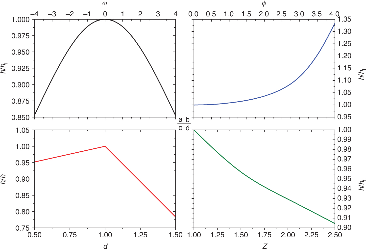
Heat transfer coefficient ratios for different values of (a) the angular velocity of the mixer ω; (b) nanoparticle volume fraction ϕ; (c) mixer size d; and (d) mixer location Z.
5 Conclusions and Future Work
To investigate the heat transfer performance and efficiency of a nanofluid-based power-law flowing through a channel into a tank with a mixer, an FEM is adopted. The walls of the tank are heated to reveal the potential of non-Newtonian power-law nanofluids in heating applications in industry. The CMC-water (0.0 %–0.4 %), a typical type of pseudoplastic power-law fluid, is considered as the base fluid. TiO2 nanoparticles are used. The influences of various parameters, such as the generalised Pr, the generalised Re, ω, ϕ, mixer size and location on the temperature and velocity field are investigated. The following results are obtained:
The absolute value of the u-velocity increases when the generalised Re increases for the enhancive kinetic energy;
Both the velocity and the temperature curves are very sensitive to the mixer angular rotational speed;
The nanofluid heating effect dominates with the particle loading parameter ϕ decreases;
The addition of nanoparticles alters the magnitude of the thermal influences on the wall temperature;
The bigger the mixer, the higher the temperatures;
The u-velocity profile will translate as the location of the mixer moves;
The trough of the temperature wave will shift as the location of the mixer changes.
In the present investigation, to improve the heat transfer of nanofluids-based power-law flow in a tank with a mixer, the applicable strategies include: reducing the rotating speed; adding more nanoparticles into the fluid; keeping the size of the mixer similar to the width of the channel; and bringing the mixer closer to the channel exit. However, adding more nanoparticles into the base fluid is considered to be the most efficient method to enhance the heat transfer coefficient of a nanofluid.
Funding source: National Natural Science Foundation of China
Award Identifier / Grant number: 11402188
Funding statement: The work of Botong Li is supported by the Fundamental Research Funds for the Central Universities (No. FRF-TP-17-020A1) and the National Natural Science Foundation of China (No. 11402188). Botong Li is very grateful to Mr. Fengbin Sun for all his support and love.
Nomenclature
- cp
fluid specific heat (J/kg ⋅ K)
- d
diameter of the mixer
- dt
time step size
- h
heat transfer coefficient (W/m2 ⋅ K)
- hf
reference heat transfer coefficient (W/m2 ⋅ K)
- i
time point
- k
thermal conductivity (W/m ⋅ K)
- L
length (m)
- n
power law index
- Pr
generalised Prandtl number (
- p
pressure (Pa)
- qi
heat flux (W/m2)
- Re
Reynolds number (
- T
temperature (K)
- u, v
velocity components along x and y directions, respectively (m/s)
- v
shape function vector (m/s)
- x, y
Cartesian coordinates along the plate and normal to it, respectively (m)
- Z
distance from the centre of the mixer to the exit of the channel
- Greek symbols
- Ω
calculation domain
- Γ
boundary of Ω
- ϕ
particle loading parameter (%)
- ρ
density of fluid (kg/m3)
- ε
penalty constant
- ω
cylinder angular velocity
- Subscripts
- nf
nanofluid
- bf
base fluid
- p
nanoparticle
References
P. R. Mashaei and M. Shahryari, Acta Astronautica 111, 345 (2015).10.1016/j.actaastro.2015.02.003Search in Google Scholar
F. Selimefendigil and H. F. Öztop, Int. J. Heat Mass Transf. 69, 54 (2014).10.1016/j.ijheatmasstransfer.2013.10.010Search in Google Scholar
S. U. S. Choi and J. A. Eastman, No. ANL/MSD/CP-84938; CONF-951135-29, Argonne National Laboratory, IL, USA, 99 1995.Search in Google Scholar
Z.-H. Liu and Y.-Y. Li, Int. J. Heat Mass Transf. 55, 6786 (2012).10.1016/j.ijheatmasstransfer.2012.06.086Search in Google Scholar
R. Sureshkumar, S. T. Mohideen, and N. Nethaji, Renew. Sustain. Energy Rev. 20, 397 (2013).10.1016/j.rser.2012.11.044Search in Google Scholar
A. Kamyar, R. Saidur, and M. Hasanuzzaman, Int. J. Heat Mass Transf. 55, 4104 ( 2012).10.1016/j.ijheatmasstransfer.2012.03.052Search in Google Scholar
M. R. Eid, J. Mol. Liq. 220, 718 (2016).10.1016/j.molliq.2016.05.005Search in Google Scholar
A. K. Sharma, A. K. Tiwari, and A. R. Dixit, Renew. Sustain. Energy Rev. 53, 779 (2016).10.1016/j.rser.2015.09.033Search in Google Scholar
M. Bahiraei and M. Alighardashi, J. Mol. Liq. 219, 117 (2016).10.1016/j.molliq.2016.03.007Search in Google Scholar
A. K. Santra, S. Sen, and N. Chakraborty, Int. J. Therm. Sci. 48, 391 (2009).10.1016/j.ijthermalsci.2008.10.004Search in Google Scholar
M. R. Eid and K. L. Mahny, Heat Transf. Asian Res. 47, 54 (2018).10.1002/htj.21290Search in Google Scholar
R. Ellahi, M. Raza, and K. Vafai, Math. Comput. Model. 55, 1876 (2012).10.1016/j.mcm.2011.11.043Search in Google Scholar
R. Ellahi, A. Zeeshan, K. Vafai, and H. U. Rahman, Proc. Inst. Mech. Eng. Part N: J. Nanoeng. Nanosyst. 225, 123 (2011).10.1243/09544054JEM2057Search in Google Scholar
R. Ellahi, Appl. Math. Model. 37, 1451 (2013).10.1016/j.apm.2012.04.004Search in Google Scholar
M. R. Eid, K. L. Mahny, T. Muhammad, and M. Sheikholeslami, Results Phys. 8, 1185 (2018).10.1016/j.rinp.2018.01.070Search in Google Scholar
A. Esmaeilnejad, H. Aminfar, and M. S. Neistanak, Int. J. Therm. Sci. 75, 76 (2014).10.1016/j.ijthermalsci.2013.07.020Search in Google Scholar
M. Hatami and D. D. Ganji, J. Mol. Liq. 188, 155 (2013).10.1016/j.molliq.2013.10.009Search in Google Scholar
M. R. Eid and K. L. Mahny, Adv. Powder Technol. 28, 3063 (2017).10.1016/j.apt.2017.09.021Search in Google Scholar
S. Baheri Islami, B. Dastvareh, and R. Gharraei, Int. J. Heat Mass Transf. 78, 917, (2014).10.1016/j.ijheatmasstransfer.2014.07.022Search in Google Scholar
H. Eshgarf and M. Afrand, Exp. Therm. Fluid Sci. 76, 221 (2016).10.1016/j.expthermflusci.2016.03.015Search in Google Scholar
N. Putra, W. Roetzel, and S. K. Das, Heat Mass Transf. 39, 775 (2003).10.1007/s00231-002-0382-zSearch in Google Scholar
M. Hojjat, S. G. Etemad, R. Bagheri, and J. Thibault, Int. J. Heat Mass Transf. 54, 1017 (2011).10.1016/j.ijheatmasstransfer.2010.11.039Search in Google Scholar
M. S. Astanina, M. A. Sheremet, H. F. Öztop, and N. Abu-Hamdeh, Int. J. Heat Mass Transf. 118, 527 (2018).10.1016/j.ijheatmasstransfer.2017.11.018Search in Google Scholar
M. K. Abdolbaqi, R. Mamat, N. A. C. Sidik, W. H. Azmi, and P. Selvakumar, Int. J. Heat Mass Transf. 108, 1026 (2017).10.1016/j.ijheatmasstransfer.2016.12.024Search in Google Scholar
W.-C. Chen and W.-T. Cheng, Int. Commun. Heat Mass Transf. 71, 208 (2016).10.1016/j.icheatmasstransfer.2015.12.020Search in Google Scholar
M. R. Eid, J. Nanofluids 6, 550 (2017).10.1166/jon.2017.1347Search in Google Scholar
F. Selimefendigil and H. F. Öztop, Comput. Fluids 109, 27 (2015).10.1016/j.compfluid.2014.12.007Search in Google Scholar
A. Alam and K.-Y. Kim, Chem. Eng. J. 181, 708 (2012).10.1016/j.cej.2011.12.076Search in Google Scholar
A. S. Kherbeet, M. R. Safaei, H. A. Mohammed, B. H. Salman, H. E. Ahmed, et al. Int. Commun. Heat Mass Transf. 76, 237 (2016).10.1016/j.icheatmasstransfer.2016.05.022Search in Google Scholar
H. Togun, M. R. Safaei, R. Sadri, S. N. Kazi, A. Badarudin, et al. Appl. Math. Comput. 239, 153 (2014).10.1016/j.amc.2014.04.051Search in Google Scholar
J. Buongiorno, J. Heat Transf. 128, 240 (2006).10.1115/1.2150834Search in Google Scholar
D. A. Nield and A. Bejan, Convection in Porous Media. Springer, New York 2006.Search in Google Scholar
S. M. H. Payam Rahim Mashaei, J. Porous Media, 17, 549, 2014.10.1615/JPorMedia.v17.i6.60Search in Google Scholar
O. A. Akbari, M. R. Safaei, M. Goodarzi, N. S. Akbar, M. Zarringhalam, et al.et al. Adv. Powder Technol. 27, 2175 (2016).10.1016/j.apt.2016.08.002Search in Google Scholar
D. X. Jin, Y. H. Wu, and J. T. Zou, Petro-Chem. Equip. 29, 7 (2000).10.1023/A:1007100411643Search in Google Scholar
M. Hojjat, S. G. Etemad, R. Bagheri, and J. Thibault, Int. Commun. Heat Mass Transf. 38, 144 (2011).10.1016/j.icheatmasstransfer.2010.11.019Search in Google Scholar
B. Li, L. Zheng, P. Lin, Z. Wang, and M. Liao, Numer. Math.: Theor. Methods Appl. 9, 315 (2016).10.4208/nmtma.2016.m1423Search in Google Scholar
B. Li, Y. Lin, L. Zhu, and W. Zhang, Appl. Therm. Eng. 94, 404 (2016).10.1016/j.applthermaleng.2015.10.148Search in Google Scholar
B. Li, W. Zhang, B. Bai, Y. Lin, and G. Kai, Microfluid. Nanofluidics 20, 154 (2016).10.1007/s10404-016-1818-ySearch in Google Scholar
B. Li, W. Zhang, L. Zhu, Y. Lin, and B. Bai, Int. J. Heat Mass Transf. 107, 836 (2017).10.1016/j.ijheatmasstransfer.2016.11.091Search in Google Scholar
H. Shi, P. Lin, B. Li, and L. Zheng, Math. Methods Appl. Sci. 37, 121 (2014).10.1002/mma.2872Search in Google Scholar
P. Lin and C. Liu, J. Comput. Phys. 215, 348 (2006).10.1016/j.jcp.2005.10.027Search in Google Scholar
E. Azhar, Z. Iqbal, and E. N. Maraj, Z. Naturforsch. A 71, 837 (2016).10.1515/zna-2016-0188Search in Google Scholar
©2018 Walter de Gruyter GmbH, Berlin/Boston
Articles in the same Issue
- Frontmatter
- General
- Noncommutativity and Relativity
- Atomic, Molecular & Chemical Physics
- Optical Ammonia Sensor Based on ZnO:Eu2+ Fluorescence Quenching Nanoparticles
- The Roles of Solute-Solute and Solute-Solvent Interactions on the Nonlinearity of Aqueous Solutions of Ionic Dyes
- Dynamical Systems & Nonlinear Phenomena
- Effect of Superthermal Polarization Force on Dust Acoustic Nonlinear Structures
- Two Integrable Classes of Emden–Fowler Equations with Applications in Astrophysics and Cosmology
- Stability and Spatiotemporal Bifurcations in Spatially Distributed Neural Networks with Nonlocal Delay
- Hydrodynamics
- Effect of Slip Velocity on the Rotating Electro-Osmotic Flow of the Power-Law Fluid in a Slowly Varying Microchannel
- Influence of Compliant Walls and Heat Transfer on the Peristaltic Transport of a Rabinowitsch Fluid in an Inclined Channel
- Solid State Physics & Materials Science
- Metal-Insulator Transition of Solid Hydrogen by the Antisymmetric Shadow Wave Function
- Investigations of Structural, Elastic, Electronic and Thermodynamic Properties of X2TiAl Alloys: A Computational Study
- Thermodynamics & Statistical Physics
- An Investigation of the Forced Convection and Heat Transfer with a Cylindrical Agitator Subjected to Non-Newtonian Nanofluids