Performance evaluation of internal quality control rules, EWMA, CUSUM, and the novel machine learning model
-
Hikmet Can Çubukçu


Abstract
Objectives
The present study set out to build a machine learning model to incorporate conventional quality control (QC) rules, exponentially weighted moving average (EWMA), and cumulative sum (CUSUM) with random forest (RF) algorithm to achieve better performance and to evaluate the performances the models using computer simulation to aid laboratory professionals in QC procedure planning.
Methods
Conventional QC rules, EWMA, CUSUM, and RF models were implemented on the simulation data using an in-house algorithm. The models’ performances were evaluated on 170,000 simulated QC results using outcome metrics, including the probability of error detection (Ped), probability of false rejection (Pfr), average run length (ARL), and power graph.
Results
The highest Pfr (0.0404) belonged to the 1–2s rule. The 1–3s rule could not detect errors with a 0.9 Ped up to 4 SD of systematic error. The random forest model had the highest Ped for systematic errors lower than 1 SD. However, ARLs of the model require the combined utility of the RF model with conventional QC rules having lower ARLs or more than one QC measurement is required.
Conclusions
The RF model presented in this study showed acceptable Ped for most degrees of systematic error. The outcome metrics established in this study will help laboratory professionals planning internal QC.
Özet
Amaç
Bu çalışma, daha iyi performans elde etmek için geleneksel kalite kontrol (KK) kurallarını, üstel ağırlıklı hareketli ortalamayı (ÜAHO) ve kümülatif toplamı (KÜTOP), rastgele orman (RO) algoritmasıyla birleştirmek için bir makine öğrenimi modeli oluşturmak ve KK prosedürü planlamasında laboratuvar uzmanlarına yardımcı olmak için bilgisayar simülasyonu kullanarak bu modellerin performanslarını değerlendirmek üzere yapılmıştır.
Yöntemler
Bir in-house algoritma kullanılarak simülasyon verileri üzerinde geleneksel KK kuralları, ÜAHO, KÜTOP ve RO modelleri uygulandı. Modellerin performansları, hata tespit olasılığı (HTO), yanlış reddetme olasılığı (YRO), ortalama çalışma uzunluğu (OÇU) ve güç grafiği dahil olmak üzere sonuç ölçüleri kullanılarak 170 000 simüle edilmiş KK sonucu üzerinde değerlendirildi.
Bulgular
En yüksek YRO (0,0404) 1–2s kuralına aitti. 1–3s kuralı, 0,9 HTO’a kadar 4 SD’ye kadar olan sistematik hataları algılayamadı. Rastgele orman modeli, 1 SD’den düşük sistematik hatalar için en yüksek HTO’na sahipti. Bununla birlikte, modelin OÇU’ları, daha düşük OÇU’larına sahip geleneksel KK kurallarıyla RO modelinin birleşik kullanımını veya birden fazla KK ölçümünü gerektirmektedir.
Sonuçlar
Bu çalışmada sunulan RO modeli, çoğu sistematik hata derecesi için kabul edilebilir HTO değerlerine sahipti. Bu çalışmada oluşturulan sonuç ölçüleri, laboratuvar profesyonellerinin iç KK planlamasına yardımcı olacaktır.
Introduction
The probability, severity, and detectability of an error constitute three pillars to be considered in risk management of clinical laboratory [1]. In addition, quality control (QC) rules are involved in the formal decision-making process, which aims to detect whether examination procedures performed in-control state or not.
The conventional QC rules such as 1–2s, 1–3s, 2–2s, 4–1s, and 10x are implemented on Shewhart’s graph, displaying QC results, the target value (mean), and multiples of standard deviation for an available time period [2]. In addition to conventional Westgard rules, trend detection rules like exponentially weighted moving average (EWMA), cumulative sum (CUSUM) help laboratory professionals to detect smaller shifts and trends [1]. Robert first presented the EWMA chart in 1959, created by calculating the weighted average of current and previous data [3]. EWMA chart is superior to Shewhart’s graph for detecting small shifts from the target value, particularly when a lower weighting factor (0.05–0.2) is used [4, 5]. Page developed the CUSUM chart in 1954 by plotting deviations of the measured values from the target value [6]. CUSUM charts can also identify small shifts more efficiently than Shewhart’s chart like EWMA charts [7]. Thus, EWMA and CUSUM charts help to detect trends before becoming substantial errors.
QC rules can be selected using the outcome metrics. The outcome metrics of QC procedures, such as the probability of error detection (Ped), probability of false rejection (Pfr), average run length (ARL), can be estimated either by assessment of retrospective data, by mathematical calculations, and by computer simulations [1]. Power graphs are also utilized to select suitable QC rules and the number of QC measurements according to measurement procedures performance [8]. The desirable Pfr should be as low as possible; however, lower Pfr may accompany lower Ped [1]. It is crucial to achieving a balance between low Pfr and high Ped to meet acceptable performance. While these metrics are important for implementing proper QC strategy according to CLSI C24ed4, only a few old-dated studies [9, 10] investigated mostly conventional rules, and one study addressed the comparison of EWMA with conventional rules [11]. Furthermore, to date, no study has investigated the implementation of machine learning algorithms in the QC practice of laboratory medicine.
The present study set out to built a machine learning model to incorporate conventional QC rules, EWMA, and CUSUM rules with a random forest algorithm to achieve better performance. Furthermore, this research aimed to evaluate the performances of the rules mentioned above and the random forest model using computer simulation to aid laboratory professionals in QC procedure planning.
Materials and methods
The present study implemented conventional internal QC rules, EWMA, and CUSUM approaches on the simulation data using an in-house algorithm written in Python 3.7.6. programming language [12] (the source code can be downloaded from: https://github.com/hikmetc/IQCAI). Figure 1 summarizes the overall study design. The simulation procedure and calculations were based on one QC measurement per run.

Study design. Step 1: Development of machine learning model, Step 2: Performance evaluation of conventional QC rules, EWMA, CUSUM and random forest model.
Conventional internal QC rules
The conventional internal QC rules defined in Table 1 were embedded in our algorithm to generate an output about the status of the QC result as 1 and 0 for out-of-control and in-control conditions, respectively.
Definitions of the internal quality control (QC) terms (1, 2).
| Conventional rules: |
| 1–2s: Reject a run exceeding 2 SD from the target (mean) value. |
| 1–3s: Reject a run exceeding 3 SD from the target (mean) value. |
| 2–2s: Reject when two consecutive results exceed 2 SD from the target (mean) value. |
| 4–1s: Reject when four consecutive results exceed 1 SD from the target (mean) value. |
| 8x: Reject when eight consecutive results are found in one side of the target (mean) value. |
| 10x: Reject when 10 consecutive results are found in one side of the target (mean) value. |
| 12x: Reject when 12 consecutive results are found in one side of the target (mean) value. |
| Trend detection rules: |
| EWMA rule: Reject a run when EWMA value exceeds control limits. |
| CUSUM rule: Reject a run when CUSUM value exceeds control limits. |
| Outcome metrics of QC: |
| Probability of error detection (PED): Defines a chance of a QC rule rejects an out-of-control condition |
| Probability of false rejection (PFR): Means a chance of a QC rule rejects an in-control process |
| Average run length (ARL): Defines the number of runs between the beginning of error introduced or the beginning of an in-control process and the QC alert. ARL includes ARLfr and ARLed |
| Average number of QC runs (events) before false rejection (ARLfr): Means the number of runs between the beginning of an in-control process and a false rejection |
| Average number of QC runs (events) required to detect out-of-control condition (ARLed): Means number of runs between the beginning of error introduced and the QC alert |
-
SD, standard deviation; EWMA, exponentially weighted moving average; CUSUM, cumulative sum.
EWMA approach
EWMA chart was constructed using the following formula [7]:
λ: Weighting factor which adjusts the weight to be given in current and previous results.
z i : ith EWMA result.
z i−1: (i − 1)th EWMA result.
x i : latest QC result.
Upper and lower control limits were determined as follows [7]:
μ=z 0: Target value (mean).
L: The factor determines the width of upper and lower control limits.
σ: Standard deviation.
If z i surpasses control limits, the process is considered out-of-control [7].
The QC procedure simulation utilized three different weighting factors (0.05, 0.1, and 0.2). The present study’s algorithm for EWMA outputs as 1 and 0 for out-of-control and in-control conditions, respectively.
CUSUM approach
CUSUM chart was applied after the standardization of QC result (x i ) with the following formula [7]:
y i : the standardized value of x i .
μ 0: Target value (mean).
σ: Standard deviation.
Standardized CUSUM values (C) for positive and negative deviations were calculated as follows, respectively [7]:
k: the reference value is regarded as 0.5.
When the CUSUM value (y i ) exceeds the default control limit (h=5), the process is considered out-of-control [7].
The algorithm for CUSUM gives the result as 1 and 0 for out-of-control and in-control conditions, respectively.
Development of machine learning model
The gaussian distributed 32,000 in-control internal QC results were generated using Python 3.7.6 [12]. with Numpy package 1.19.1 [13]. Simulation results were produced using the mean as 4.5 and standard deviation as 0.06. Systematic errors corresponding to 0.25, 0.50, 0.75, 1.0, 1.25, 1.50, 1.75, 2.0, 2.25, 2.50, 2.75, 3.0, 3.25, 3.50, 3.75, and 4.0 multiples of standard deviations were introduced to the half of the 32,000 results (n=16,000, 1,000 results for each degree of systematic error).
Conventional QC rules (including 1–2s, 1–3s, 2–2s, 4–1s, 8x, 10x, and 12x), EWMA, and CUSUM rules were implemented on the above-mentioned 32,000 internal QC results, and the outputs were recorded as 1 and 0 for out-of-control and in-control conditions, respectively. The output results of QC rules were utilized as input variables and the presence of an error as the target variable for the machine learning model (Figure 1, Step 1).
A total of 32,000 output results were split into training and test data sets using 80 and 20% of the overall data, respectively. The training data set was used to built the machine learning model using the random forest algorithm and for ten-fold cross-validation [14] to evaluate the model’s generalizable performance in terms of accuracy. The random forest classifier model used 200 decision trees, entropy for information gain, and other default parameters based on the scikit-learn 0.24.1 package [15, 16] (the source code can be downloaded from: https://github.com/hikmetc/IQCAI). Hyperparameter optimization was not performed. The random forest model’s performance was assessed using the test set with sensitivity, specificity, accuracy, and receiver operating characteristic (ROC) curve analysis.
Performance evaluation of conventional QC rules, EWMA, CUSUM and random forest model
According to CLSI C24ed4, computer simulations and power graphs are required to evaluate QC rules performance. The Ped, Pfr, and ARL are considered crucial outcome metrics for internal QC rule evaluation [1]. Therefore, the external performance evaluation of the random forest model and general performance evaluation of conventional QC rules, EWMA, and CUSUM approaches were performed using the outcome metrics and power graph (Figure 1, Step 2).
The overall performances of the QC rules, EWMA, CUSUM, and random forest model were evaluated on the total number of 170,000 simulated QC results consist of in-control and out-of-control conditions. This data was independent of the train data set used for the random forest model’s training. Systematic errors corresponding to 0.25, 0.50, 0.75, 1.0, 1.25, 1.50, 1.75, 2.0, 2.25, 2.50, 2.75, 3.0, 3.25, 3.50, 3.75, and 4.0 multiples of standard deviations introduced separately to on Gaussian distributed in-control simulation data to achieve out-of-control condition. The Ped and ARL were calculated after adding each degree of systematic error to the in-control results (1,000 in-control results followed by 1,000 out-of-control results in each systematic error simulation). While run-length values were determined by subtracting the order of the first rejection signal from the beginning of the out-of-control results, the frequency of rejection signal among out-of-control results yielded a probability of error detection. Then, the out-of-control result simulation was repeated 10 times, and average values of Ped and run-length were recorded ((10 × 1,000) × 16 degrees of systematic errors).
The Pfr values were determined from the data, including 10,000 in-control QC results (Pfr=number of false rejection signal/total in-control QC results). Then, the power graph was formed using Ped and Pfr values of QC.
The QC rules corresponding to the Ped of ≥0.9 were regarded as acceptable for an intended degree of systematic error [2]. The probability of ≤0.05 was considered acceptable for false rejection [2].
The outcome metrics were calculated by the in-house Python code (https://github.com/hikmetc/IQCAI). The power graph was drawn using GraphPad Prism version 9 (San Diego, USA).
Results
The random forest model’s performance characteristics on the initial test data set (n: 6,400) are given in supplementary material and Table 2. The accuracy from tenfold cross-validation was 95.79% ± 0.23%.
Sensitivity, specificity, positive predictive value, negative predictive value, accuracy values determined from test data set (n=6,400). tenfold cross validation accuracy value determined from train data set (n=25,600).
| Statistic | Value | 95% CI |
|---|---|---|
| Sensitivity | 92.04% | 91.05–92.96% |
| Specificity | 99.53% | 99.23–99.74% |
| Positive predictive value | 99.49% | 99.16–99.69% |
| Negative predictive value | 92.58% | 91.73–93.35% |
| Accuracy | 95.78% | 95.26–96.26% |
| Tenfold cross validation accuracy (mean ± SD) | 95.79% ± 0.23% |
-
CI, confidence interval.
Pfr and Ped of IQC rules, EWMA, CUSUM, and Random Forest Model are shown in Table 3. While lower ARL and Pfr values are preferred for QC rules, optimum Ped should be as high as possible. The highest Pfr (0.0404) belonged to the 1–2s rule. On the other hand, the 12x rule had the lowest Pfr (0.0004). Pfr and Ped for different degrees of systematic errors were represented in the power graph shown in Figure 2. The random forest model had the highest Ped for systematic errors lower than 1 SD.
Probability of false rejection and probability of error detection of IQC rules, EWMA, CUSUM, and random forest model.
| Systematic error (multiples of SD) | 1–2s | 1–3s | 2–2s | 4–1s | 10x | 8x | 12x | EWMA λ=0.2 | EWMA λ=0.1 | EWMA λ=0.05 | CUSUM | Random forest | Probability type |
|---|---|---|---|---|---|---|---|---|---|---|---|---|---|
| 0 | 0.0404 | 0.0018 | 0.0018 | 0.0004 | 0.0018 | 0.0144 | 0.0004 | 0.0016 | 0.0026 | 0.0044 | 0.0120 | 0.0048 | Pfr |
| 0.25 | 0.043 | 0.002 | 0.002 | 0.003 | 0.011 | 0.035 | 0.006 | 0.018 | 0.057 | 0.166 | 0.107 | 0.178 | Ped |
| 0.5 | 0.063 | 0.007 | 0.004 | 0.007 | 0.030 | 0.089 | 0.016 | 0.074 | 0.276 | 0.722 | 0.841 | 0.890 | Ped |
| 0.75 | 0.109 | 0.016 | 0.012 | 0.015 | 0.071 | 0.122 | 0.041 | 0.211 | 0.639 | 0.958 | 0.983 | 0.984 | Ped |
| 1 | 0.158 | 0.027 | 0.024 | 0.047 | 0.145 | 0.259 | 0.083 | 0.489 | 0.932 | 0.990 | 0.991 | 0.991 | Ped |
| 1.25 | 0.227 | 0.043 | 0.056 | 0.084 | 0.264 | 0.392 | 0.195 | 0.777 | 0.987 | 0.993 | 0.993 | 0.994 | Ped |
| 1.5 | 0.312 | 0.071 | 0.100 | 0.188 | 0.482 | 0.603 | 0.411 | 0.926 | 0.993 | 0.992 | 0.994 | 0.994 | Ped |
| 1.75 | 0.404 | 0.109 | 0.165 | 0.328 | 0.667 | 0.755 | 0.609 | 0.978 | 0.994 | 0.993 | 0.995 | 0.994 | Ped |
| 2 | 0.492 | 0.158 | 0.245 | 0.478 | 0.808 | 0.864 | 0.769 | 0.996 | 0.995 | 0.994 | 0.996 | 0.995 | Ped |
| 2.25 | 0.579 | 0.227 | 0.338 | 0.594 | 0.895 | 0.926 | 0.873 | 0.997 | 0.996 | 0.996 | 0.996 | 0.996 | Ped |
| 2.5 | 0.670 | 0.312 | 0.451 | 0.754 | 0.949 | 0.963 | 0.939 | 0.998 | 0.997 | 0.996 | 0.997 | 0.996 | Ped |
| 2.75 | 0.760 | 0.404 | 0.579 | 0.854 | 0.971 | 0.979 | 0.965 | 0.998 | 0.997 | 0.997 | 0.998 | 0.997 | Ped |
| 3 | 0.835 | 0.492 | 0.697 | 0.924 | 0.991 | 0.993 | 0.988 | 0.997 | 0.997 | 0.996 | 0.997 | 0.996 | Ped |
| 3.25 | 0.885 | 0.579 | 0.781 | 0.961 | 0.992 | 0.994 | 0.990 | 0.998 | 0.998 | 0.997 | 0.998 | 0.998 | Ped |
| 3.5 | 0.935 | 0.670 | 0.873 | 0.968 | 0.991 | 0.993 | 0.989 | 0.998 | 0.997 | 0.997 | 0.998 | 0.997 | Ped |
| 3.75 | 0.964 | 0.760 | 0.928 | 0.988 | 0.991 | 0.993 | 0.989 | 0.998 | 0.998 | 0.997 | 0.998 | 0.997 | Ped |
| 4 | 0.982 | 0.835 | 0.964 | 0.996 | 0.991 | 0.993 | 0.989 | 0.998 | 0.998 | 0.997 | 0.998 | 0.997 | Ped |
-
IQC, internal quality control; EWMA, exponentially weighted moving average; CUSUM, cumulative sum; λ, weighting factor of EWMA; Pfr, probability of false rejections; Ped, Probability of error detection; SD, standard deviation.

Power graph of EWMA, CUSUM, IQC rules and random forest model.
Table 4 presents ARL values of internal QC rules, EWMA, CUSUM, and Random Forest Model. The lowest average number of QC runs (events) before false rejection (ARLfr) (25) belonged to the 1–2s rule, and the highest ARLfr (1,059) was detected for the 4–1s rule. Figure 3 shows that the lowest average number of QC runs (events) required to detect out-of-control condition (ARLed) values belonged to the 1–2s rule for all degrees of systematic errors.
Average run length (ARL) of IQC rules, EWMA, CUSUM and random forest model.
| Average run length | |||||||||||||
|---|---|---|---|---|---|---|---|---|---|---|---|---|---|
| Systematic error (multiples of SD) | 1–2s | 1–3s | 2–2s | 4–1s | 10x | 8x | 12x | EWMA λ=0.2 | EWMA λ=0.1 | EWMA λ=0.05 | CUSUM | Random forest | ARL type |
| 0 | 25 | 463 | 803 | 1,059 | 940 | 109 | 3,154 | 675 | 904 | 336 | 374 | 724 | ARLfr |
| 0.25 | 25 | 408 | 667 | 605 | 337 | 63 | 606 | 173 | 120 | 77 | 124 | 57 | ARLed |
| 0.5 | 12 | 153 | 238 | 195 | 106 | 34 | 239 | 34 | 31 | 32 | 39 | 32 | ARLed |
| 0.75 | 10 | 60 | 84 | 52 | 41 | 21 | 62 | 18 | 15 | 17 | 17 | 16 | ARLed |
| 1 | 6 | 48 | 30 | 29 | 17 | 15 | 31 | 8 | 9 | 10 | 9 | 9 | ARLed |
| 1.25 | 4 | 26 | 22 | 11 | 14 | 10 | 23 | 6 | 6 | 7 | 7 | 6 | ARLed |
| 1.5 | 4 | 20 | 20 | 9 | 11 | 8 | 19 | 7 | 7 | 9 | 6 | 6 | ARLed |
| 1.75 | 5 | 10 | 11 | 7 | 10 | 8 | 12 | 6 | 6 | 8 | 6 | 6 | ARLed |
| 2 | 2 | 6 | 6 | 7 | 12 | 10 | 15 | 4 | 5 | 6 | 4 | 5 | ARLed |
| 2.25 | 2 | 5 | 6 | 5 | 9 | 7 | 11 | 3 | 4 | 5 | 4 | 4 | ARLed |
| 2.5 | 1 | 4 | 3 | 4 | 9 | 7 | 11 | 3 | 3 | 4 | 3 | 4 | ARLed |
| 2.75 | 1 | 2 | 3 | 4 | 9 | 7 | 11 | 2 | 3 | 3 | 2 | 3 | ARLed |
| 3 | 1 | 3 | 3 | 4 | 9 | 7 | 12 | 3 | 3 | 4 | 3 | 4 | ARLed |
| 3.25 | 1 | 1 | 2 | 3 | 9 | 7 | 11 | 2 | 2 | 3 | 2 | 3 | ARLed |
| 3.5 | 1 | 2 | 2 | 4 | 9 | 7 | 11 | 2 | 3 | 3 | 2 | 3 | ARLed |
| 3.75 | 1 | 1 | 2 | 4 | 9 | 7 | 11 | 2 | 2 | 3 | 2 | 3 | ARLed |
| 4 | 1 | 1 | 2 | 4 | 9 | 7 | 11 | 2 | 2 | 3 | 2 | 3 | ARLed |
-
SD, standard deviation; IQC, internal quality control; EWMA, exponentially weighted moving average; CUSUM, cumulative sum; λ, weighting factor of EWMA; ARLfr, average number of QC runs (events) before false rejection; ARLed, average number of QC runs (events) required to detect out-of-control condition.
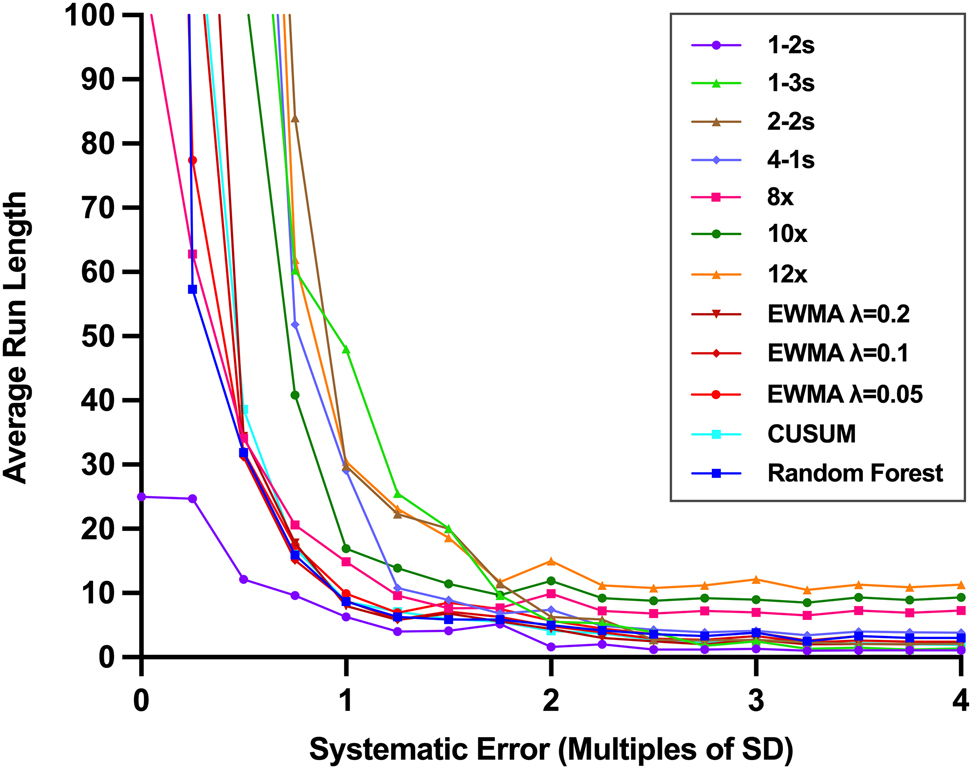
Average run length graph of EWMA, CUSUM, IQC rules and random forest model.
Discussion
The in-house code using the random forest algorithm successfully incorporated conventional internal QC rules, EWMA, and CUSUM. The error detection performance of the random forest model was found to be successful, especially for small systematic errors (<1 SD). The error detection, false rejection, and average response metrics of conventional QC rules, EWMA, CUSUM, and the novel model were extensively presented. All of the QC models were able to achieve acceptable Pfr (<0.05) for one QC measurement per run. However, the current study simulated only one QC measurement per run, and the Pfr values will double and triple in the case of two and three QC measurements per run, respectively [2]. As illustrated in Figure 2, while QC rules like 2–2s and 1–3s were suitable for detecting larger systematic errors, random forest, CUSUM, and EWMA approaches could identify smaller systematic errors or trends.
In the present study, the 1–2s rule showed the highest Pfr (0.04). Thus, 1 out of every 25 QC results revealed false rejection with the 1–2s rule (Table 3). Additionally, when the 1–2s rule is applied to 25 different tests, it can be assumed that 1 test will be rejected every day. The desirable QC rule’s Pfr should be as low as possible [1]. Therefore, the 1–2s rule should be implemented cautiously. Surprisingly, Rosenbaum et al. [17] reported that 16 out of 21 clinical laboratories of the USA’s reputed academic centers used only 2 SD rule. Figure 3 and Table 4 showed that the 1–2s rule had the lowest ARLfr and ARLed values. The possible motivation for 1–2s rule usage [17] might be these low ARL values, resulting in frequent QC alerts as warnings in daily practices. Nevertheless, the Ped of 1–2s rule was lower than 8x, 10x, 12x, EWMA, CUSUM, and random forest model for most of the degrees of systematic error. Thus, the 1–2s rule should be considered as a warning alert or be used in a multirule scheme.
The 1–3s rule could not detect errors with a 0.9 probability of error detection up to 4 SD of systematic error (Table 3, Figure 2) despite its acceptable Pfr (0.0018). Hence, the 1–3s rule was not sufficient for stand-alone usage. The 2–2s rule had a similar Pfr with the 1–3s rule. However, the 2–2s rule’s Ped was higher than the 1–3s rule for the systematic errors higher than 1 SD (Table 3, Figure 2). The 4–1s rule was able to identify the systematic error of 3 SD with higher than 0.9 Ped. However, as shown in Table 4, the ARL value of the 4–1s rule for large systematic errors (3–4 SD) was 4, which may lead to a lag in stand-alone usage.
Although 8x, 10x, and 12x rules showed acceptable Ped for systematic errors higher than 2.25 SD (Table 3), ARL values were 7, 9, and 11 for 8x, 10x, and 12x rules, respectively (Table 4). Thus, these rules were not sufficient for detecting larger errors like 2 SD or more individually. On the other hand, Ped values of 8x, 10x, and 12x rules were unacceptable (<0.9) for the systematic errors lower than 2 SD (Table 3, Figure 2). These findings showed that 8x, 10x, and 12x rules were inefficient when utilized individually for the statistical QC procedure.
The weighting factor constitutes the backbone of the EWMA approach. Linnet modified the EWMA approach using 2 and 3 SD as control limits and 0.5 as the weighting factor. This modified EWMA approach outperformed conventional QC rules and multirules for detecting larger errors such as 2 SD [11]. However, original control limits and weighting factors of 0.2, 0.1, and 0.05 were utilized in the present study to fit for its purpose of detecting trends and small systematic errors [5]. Overall, Pfr values were quite low for EWMA approaches, regarding the acceptable limit of 0.05. The Ped values from highest to lowest belonged to EWMA (λ=0.05), EWMA (λ=0.1), and EWMA (λ=0.2), respectively (Table 3, Figure 2). Hence, the EWMA approach using λ value of 0.05 was able to detect lower systematic errors with acceptable performance compared to other λ values (Figure 2).
As shown in Figure 2, the CUSUM approach’s performance was acceptable for identifying small systematic errors like the EWMA approach (Figure 2). On the other hand, the Pfr value of CUSUM (0.012) was higher than the Pfr values of EWMA (0.0016–0.0044) and the Random forest model (0.0048) (Table 3). Westgard et al. [18] showed that the combined usage of CUSUM and Shewhart charts enhanced Ped. Furthermore, the combined utility of EWMA and Shewhart chart (conventional QC rules) was recommended previously [19] due to the inertia effect that leads to a lag in error detection, particularly when a lower weighting factor is used [7]. Likewise, in the present study, EWMA and CUSUM approaches could not detect substantially large systematic errors such as 3 SD with one QC measurement per run, as inferred from ARLed values (Table 4). Thus, laboratory professionals should consider the ARL values when combining different QC procedures and determining the number of QC measurements while preserving acceptable limits of Pfr. For instance, the Pfr value of CUSUM is 0.012; thus, the remainder Pfr of 0.038 can be reserved for other rules having lower ARLed while preserving acceptable Pfr (0.05). The remaining Pfr can also be reserved for rules that can detect random errors. For example, a laboratory professional may intend to detect systematic errors higher than 1.5 SD and substantial random errors, in this case, EWMA (λ=0.2) may be preferred for preserving Ped ≥0.9, and may combine with the “1–3s” rule which can cover random errors [20] while maintaining Pfr ≤0.05.
The random forest model showed the best Ped for 0.25 SD, 0.5 SD, and 0.75 SDs of systematic errors. The Ped values for systematic errors equal to or higher than 1 SD were similar to EWMA (λ=0.05) and CUSUM approaches (Table 3). In addition, Ped values of the random forest model were acceptable for systematic errors higher than 0.5 SD while preserving acceptable Pfr (0.0048). However, ARLed values did not let the random forest model be used individually for one QC measurement per the run scheme, as shown in Table 4. Therefore, the random forest model should be used in combination with other conventional QC rules having lower ARLed for large systematic errors, or more than one QC measurement per run is required regarding ARLed values.
The CUSUM approach had the highest feature importance among the input variables of the random forest model, followed by EWMA (λ=0.05) and EWMA (λ=0.1) (Figure 4). In contrast, the 4–1s rule had the lowest importance for the random forest model to predict systematic error (Figure 4). Therefore, it can be suggested that CUSUM and EWMA approaches are preferably included in the internal QC procedure to detect systematic analytical errors even if the machine learning model is not used.

Feature importance chart of random forest model.
According to CLSI C24ed4, procedures with quite good analytical performance regarding their medical needs may be tracked with less strict QC rules like 4–1s and 1–3s. On the other hand, procedures having marginal performance may need a combination of QC rules [1]. The error detection ability of QC rules varies in magnitude and type of an out-of-control condition. While rules like 2–2s and 1–3s are useful to detect larger shifts, trend detection rules such as EWMA and CUSUM aid in detecting smaller shifts and trends [1]. Although most laboratories implement simple rules such as 2 SD in daily practices [17], with the evolution of technology and computer science, implementation of multiple QC procedures and state-of-art tools like machine learning models have become applicable.
This is the first study implementing a machine learning model as an internal QC rule in laboratory medicine. The source codes and the developed random forest model were also shared publicly (https://github.com/hikmetc/IQCAI). The present study also provided an extensive performance evaluation of well-known internal QC rules, which had been investigated by only a few studies [9], [10], [11]. The Pfr values of 1–2s and 1–3s were reported as 0.049 and 0.0020 by Westgard et al. [10] and 0.089 and 0.0054 by Parvin [21], respectively. In addition, the latter study reported higher Ped values of these rules than the present study. However, 2 SD covers at least 95% of the Gaussian distributed results and does not conform with the Pfr higher than 0.05 for the 1–2s rule. Nevertheless, the present study provides source codes of the simulation to maintain its reproducibility. The outcome metrics established in this study will help laboratory professionals planning internal QC procedures. It should be kept in mind that while EWMA, CUSUM, and the novel random forest model can detect small systematic errors or trends with their higher Ped, this ability may lead to frequent interruption due to small but not clinically substantial errors in the daily laboratory routine. Therefore, laboratory professionals may prefer to choose a strategy between detecting small shifts before becoming substantial errors or detecting only substantial errors using conventional rules like 1–3s and 2–2s.
The present study was limited by the absence of the multirules’ performance evaluation. Multirules are formed by the combined utility of conventional QC rules and were not compared with the random forest model presented in this study. Linnet demonstrated that the EWMA approach had better performance than multirules [11]. While we showed that the random forest model outperformed EWMA approaches, the weighting factor and control limits used in the present study differed from Linnet’s. Thus, further research is needed to address the concomitant comparison of multirules, EWMA, CUSUM, and random forest models. The second limitation was that the present study simulated only one QC measurement per run scenario. Assuming different concentration levels are tested in the internal QC procedure, further studies about higher numbers of QC measurements need to be conducted. Another limitation was that only systematic errors were simulated in the present study. Laboratory professionals face random errors in daily routine; therefore, more research is needed to investigate both random and systematic errors for conventional QC rules, EWMA, CUSUM, and random forest models.
Conclusions
The random forest model presented in this study showed acceptable Ped for most degrees of systematic error. However, the ARL values of the model require the combined utility of the random forest model with conventional QC rules having lower ARL values or more than one QC measurement is required. The present study has reported extensive outcome metrics of internal QC procedures, which may help laboratory professionals plan their procedure with acceptable Ped and Pfr values.
-
Conflict of interest: The author declares no conflict of interest.
Ped calculation for the multi-rule scheme:
Ped: Probability of error detection.
Pfr: Probability of false rejection
Note: The ARL value is related to the response time of QC rules. Therefore, the ARL value of a multi-rule scheme would be the minimum ARL among the combined rules.
Example:
Objective: to detect systematic errors higher than 1.5 SD with Ped >0.9 and Pfr <0.05 and to determine systematic errors >3 SD with ARL of 1.
Ped values of EWMA are higher than 0.9 for systematic errors ≥1.5 SD; thus, the combined Ped will be higher than 0.9.
For 1.5 of systematic error, combined Ped would be:
For 1.25 of systematic error, combined Ped would be:
The minimum ARL value for systematic errors >3 SD among 1–3s rule and EWMA (λ=0.2) is 1, which belongs to the 1–3s rule (Table 4).
Overall, the present scheme could detect systematic errors >3 SD with 1 ARL and determine systematic errors ≥1.5 SD with Ped >0.9 while preserving Pfr <0.05.
References
1. CLSI. Statistical quality control for quantitative measurement procedures: principles and definitions. CLSI guideline C24, 4th ed. Wayne, Pennsylvania, USA: Clinical and Laboratory Standards Institute; 2016.Search in Google Scholar
2. Westgard, JO. Internal quality control: planning and implementation strategies. Ann Clin Biochem 2003 Nov;40:593–611 [Epub 2003/11/25]. https://doi.org/10.1258/000456303770367199.Search in Google Scholar PubMed
3. Lucas, JM, Saccucci, MS. Exponentially weighted moving average control schemes: properties and enhancements. Technometrics 1990;32:1–12. https://doi.org/10.1080/00401706.1990.10484583.Search in Google Scholar
4. Carson, PK, Yeh, AB. Exponentially weighted moving average (EWMA) control charts for monitoring an analytical process. Ind Eng Chem Res 2008;47:405–11. https://doi.org/10.1021/ie070589b.Search in Google Scholar
5. Çubukçu, HC. The weighting factor of exponentially weighted moving average chart. Turk J Biochem 2020;45:639–41.10.1515/tjb-2019-0368Search in Google Scholar
6. Page, ES. Continuous inspection schemes. Biometrika 1954;41:100–15. https://doi.org/10.2307/2333009.Search in Google Scholar
7. Montgomery, DC. Introduction to statistical quality control, 7th ed. Danvers: John Wiley & Sons; 2013.Search in Google Scholar
8. Westgard, JO. Useful measures and models for analytical quality management in medical laboratories. Clin Chem Lab Med 2016 Feb;54:223–33 [Epub 2015/10/02]. https://doi.org/10.1515/cclm-2015-0710.Search in Google Scholar PubMed
9. Westgard, JO, Groth, T. Power functions for statistical control rules. Clin Chem 1979 Jun;25:863–9 [Epub 1979/06/01]. https://doi.org/10.1093/clinchem/25.6.863.Search in Google Scholar
10. Westgard, JO, Groth, T, Aronsson, T, Falk, H, de Verdier, CH. Performance characteristics of rules for internal quality control: probabilities for false rejection and error detection. Clin Chem 1977 Oct;23:1857–67 [Epub 1977/10/01]. https://doi.org/10.1093/clinchem/23.10.1857.Search in Google Scholar
11. Linnet, K. The exponentially weighted moving average (EWMA) rule compared with traditionally used quality control rules. Clin Chem Lab Med 2006;44:396–9 [Epub 2006/04/08]. https://doi.org/10.1515/cclm.2006.077.Search in Google Scholar
12. Van Rossum, G, Drake, FL. Python 3 reference manual. Scotts Valley, CA: CreateSpace; 2009.Search in Google Scholar
13. Harris, CR, Millman, KJ, van der Walt, SJ, Gommers, R, Virtanen, P, Cournapeau, D, et al.. Array programming with NumPy. Nature 2020 Sep;585:357–62 [Epub 2020/09/18]. https://doi.org/10.1038/s41586-020-2649-2.Search in Google Scholar PubMed PubMed Central
14. Kim, J-H. Estimating classification error rate: repeated cross-validation, repeated hold-out and bootstrap. Comput Stat Data Anal 2009;53:3735–45. https://doi.org/10.1016/j.csda.2009.04.009.Search in Google Scholar
15. Breiman, L. Random forests. Mach Learn 2001;45:5–32. https://doi.org/10.1023/a:1010933404324.10.1023/A:1010933404324Search in Google Scholar
16. Pedregosa, F, Varoquaux, G, Gramfort, A, Michel, V, Thirion, B, Grisel, O, et al.. Scikit-learn: machine learning in Python. J Mach Learn Res 2011;12:2825–30.Search in Google Scholar
17. Rosenbaum, MW, Flood, JG, Melanson, SEF, Baumann, NA, Marzinke, MA, Rai, AJ, et al.. Quality control practices for chemistry and immunochemistry in a Cohort of 21 large academic medical centers. Am J Clin Pathol 2018 Jul 3;150:96–104 [Epub 2018/06/01]. https://doi.org/10.1093/ajcp/aqy033.Search in Google Scholar PubMed
18. Westgard, JO, Groth, T, Aronsson, T, de Verdier, CH. Combined Shewhart-cusum control chart for improved quality control in clinical chemistry. Clin Chem 1977 Oct;23:1881–7 [Epub 1977/10/01]. https://doi.org/10.1093/clinchem/23.10.1881.Search in Google Scholar
19. Woodall, WH, Mahmoud, MA. The inertial properties of quality control charts. Technometrics 2005;47:425–36. https://doi.org/10.1198/004017005000000256.Search in Google Scholar
20. Kinns, H, Pitkin, S, Housley, D, Freedman, DB. Internal quality control: best practice. J Clin Pathol 2013 Dec;66:1027–32 [Epub 2013/09/28]. https://doi.org/10.1136/jclinpath-2013-201661.Search in Google Scholar PubMed
21. Parvin, CA, Kuchipudi, L, Yundt-Pacheco, JC. Should I repeat my 1:2s QC rejection? Clin Chem 2012 May;58:925–9 [Epub 2012/02/24]. https://doi.org/10.1373/clinchem.2011.181818.Search in Google Scholar PubMed
Supplementary Material
The online version of this article offers supplementary material (https://doi.org/10.1515/tjb-2021-0199).
© 2021 Hikmet Can Çubukçu, published by De Gruyter, Berlin/Boston
This work is licensed under the Creative Commons Attribution 4.0 International License.
Articles in the same Issue
- Frontmatter
- Review Article
- Overview of COVID-19’s relationship with thrombophilia proteins
- Research Articles
- Is it possible to determine antibiotic resistance of E. coli by analyzing laboratory data with machine learning?
- Detection of circulating prostate cancer cells via prostate specific membrane antigen by chronoimpedimetric aptasensor
- Two approaches for measurement uncertainty estimation: which role for bias? Complete blood count experience
- Is there any relationship between C-reactive protein/albumin ratio and clinical severity of childhood community-acquired pneumonia
- Comparison of nitric oxide and adrenomedullin levels of children with attention deficit hyperactivity disorder and anxiety disorder
- Performance evaluation of internal quality control rules, EWMA, CUSUM, and the novel machine learning model
- Are serum molecular markers more effective than the invasive methods used in the diagnosis of breast cancers?
- HIF-1 inhibitors: differential effects of Acriflavine and Echinomycin on tumor associated CA-IX enzyme and VEGF in melanoma
- Evaluation of BD Vacutainer Eclipse and BD Vacutainer Ultra-Touch butterfly blood collecting sets in laboratory testing
- The effects of various strength training intensities on blood cardiovascular risk markers in healthy men
- Is there any relationship between LGALS3 gene variations and histopathological criteria in laryngeal squamous cell carcinoma (LSCC)?
- Expression levels of BAP1, OGT, and YY1 genes in patients with eyelid tumors
- Association of bitter and sweet taste gene receptor polymorphisms with dental caries formation
- Case Report
- Glucose-6-phosphate dehydrogenase gene Ala365Thr mutation in an Iraqi family with confusing clinical differences
- Acknowledgment
- Acknowledgment