Posterior Manifolds over Prior Parameter Regions: Beyond Pointwise Sensitivity Assessments for Posterior Statistics from MCMC Inference
-
Liana Jacobi
 ,
Chun Fung Kwok
,
Chun Fung Kwok
 ,
Andrés Ramírez-Hassan
,
Andrés Ramírez-Hassan

Abstract
Increases in the use of Bayesian inference in applied analysis, the complexity of estimated models, and the popularity of efficient Markov chain Monte Carlo (MCMC) inference under conjugate priors have led to more scrutiny regarding the specification of the parameters in prior distributions. Impact of prior parameter assumptions on posterior statistics is commonly investigated in terms of local or pointwise assessments, in the form of derivatives or more often multiple evaluations under a set of alternative prior parameter specifications. This paper expands upon these localized strategies and introduces a new approach based on the graph of posterior statistics over prior parameter regions (sensitivity manifolds) that offers additional measures and graphical assessments of prior parameter dependence. Estimation is based on multiple point evaluations with Gaussian processes, with efficient selection of evaluation points via active learning, and is further complemented with derivative information. The application introduces a strategy to assess prior parameter dependence in a multivariate demand model with a high dimensional prior parameter space, where complex prior-posterior dependence arises from model parameter constraints. The new measures uncover a considerable prior dependence beyond parameters suggested by theory, and reveal novel interactions between the prior parameters and the elasticities.
1 Introduction
Bayesian inference plays an increasingly important role in empirical research across many fields including economics and related areas. A common application requires the specification of a potentially large set of location and precision parameters (henceforth referred to as prior parameters) for prior distributions that have been predetermined based on modelling aspects and computational efficiency (i.e. prior conjugacy). It is well known that prior parameter choices can lead to a prior dependence of the posterior statistics (Berger 1990) and they should be carefully chosen (Lancaster 2004). This paper introduces a new approach that assesses prior parameter dependence via the functions of the posterior statistics over relevant prior parameter regions (sensitivity manifolds) with the aim to expand upon commonly used localized strategies. We propose a computational strategy for settings where inference is based on efficient MCMC methods that opens up possibilities of a more comprehensive analysis of prior dependence patterns through a range of new numerical and graphical measures. For example, it allows the identification of prior parameters with the largest impacts on posterior estimates of key statistics, as well as to identify those posterior statistics that are particularly sensitive to prior parameter specifications (within a region in the prior parameter space).
By design, analysis of prior parameter dependence differs in focus from the broader set of issues in the well-established and large literature on Bayesian robustness (Berger 1985; Bhatia et al. 2023; Giacomini, Kitagawa, and Read 2022; Li and Dunson 2020; Ríos Insua, Ruggeri, and Martín 2000; Ruggeri 2008). The main objective of the former is in assessing changes in posterior inference when moving away from an initial point within the prior parameter space for a given model (likelihood) and prior distribution. For example in the context of sparse modelling in macroeconomic time series analysis with prior shrinkage, several studies have looked on the impacts of widely used shrinkage parameters (Amir-Ahmadi, Matthes, and Wang 2020; Chan, Jacobi, and Zhu 2022; Jarociński and Marcet 2019). In practice, researchers typically investigate the impact of prior parameter assumptions on posterior statistics in terms of local or pointwise assessments. This has been done in the form of partial derivatives (see for example Giordano et al. 2022; Gustafson 2000; Jacobi, Zhu, and Joshi 2022) or, more often, in terms of multiple evaluations under a restricted set of alternative prior parameter specifications popularized by Richardson and Green (1997).
Both the design and analytical and computational complexity of the posterior inference limit the possible scope of such approaches. For example, the popular “scenario” type perturbation (or multi-evaluation) analysis evaluates posterior statistics at a few additional sets of prior parameter specifications from perturbing the initial parameter setting (An and Schorfheide 2007; Kim and Nelson 1999; Richardson and Green 1997). An additional limitation is the exogenous choice of these additional evaluation points in the prior parameter space, mostly ad hoc and without any reference to the posterior surface, at most supported by prior simulations (Del Negro and Schorfheide 2008) or modelling aspects (Chan, Jacobi, and Zhu 2019; Giannone, Lenza, and Primiceri 2015). Following a different strategy, local derivative approaches consider the impact of a one-directional infinitesimal change away from an initial point in the prior parameter space on posterior statistics (Gustafson 2000). The required analytical derivative expressions are commonly intractable, although several papers have discussed computational approaches to obtain derivative estimates for posterior mean parameters and with respect to a subset of hyperparameters in specific parametric classes (Basu, Jammalamadaka, and Liu 1996; Geweke 1999; Müller 2012; Pérez, Martin, and Rufo 2006).
This paper expands upon common localized strategies by developing comprehensive formal measures and graphical assessments of prior parameter dependence based on the graph of a posterior statistic over regions in the prior parameter space (sensitivity manifolds). For example, sensitivity manifolds allow for the computation of a broader sensitivity measure that relates to the global results measure (Berger 1990). Importantly, information based on the geometry properties of these posterior surfaces can capture aspects of prior parameter dependence beyond available pointwise and local assessments, including policy turning points and joint-influence of multiple prior parameters, that are particularly relevant in empirical applications.
Analytical expressions for the sensitivity manifold, a function of a posterior statistic over a region in the prior parameter space, are only available in a few simple cases as in the Bernoulli example used as an illustration below. For MCMC settings, such a multivariate demand analysis as considered in our application, we propose an innovative computational strategy based on Gaussian Processes (GP) methods (Rasmussen and Williams 2006) with an extension to combine GP estimation with derivative information obtained via a computation approach for MCMC inference (Jacobi, Zhu, and Joshi 2022). Our approach builds on recent convergence results for GP in the context of posterior inference (Stuart and Teckentrup 2018) and contributes to the recent literature on the use of GP-based methods in Bayesian inference (see for example work on GP priors in Branson et al. (2019), Clark et al. (2022), Hauzenberger et al. (2021)). To achieve both precision and efficiency for the sensitivity manifold estimation with MCMC evaluations, we employ a GP-based strategy that is based on multiple point evaluations under the GP that is combined with efficient selection of evaluation points via Active Learning (Settles 2012).
Derivative information, if available, can be readily included within such a GP-based estimation framework since the derivative of a GP itself takes the form of a GP. In addition to improving the precision of the GP approximation of the manifolds, and reducing computational load as less evaluation points are required (see example below), such derivative information supports additional sensitivity measures. As we illustrate in our application, it also affords a more informative use manifold-based sensitivity analysis of particular relevance in settings with higher-dimensional prior parameter space where many prior parameters can potentially drive prior dependence of inference. To realize these benefits, we exploit a novel approach for unbiased estimation of derivatives of posterior statistics formalized in Jacobi, Zhu, and Joshi (2022) that can be efficiently estimated via the vectorized automatic differentiation approach (Kwok, Zhu, and Jacobi 2020), implemented in the context of Bayesian VAR analysis with shrinkage priors (Chan, Jacobi, and Zhu 2020, 2022).
We apply the new approach and methods in the context of the estimation of food demand elasticities in a widely used multivariate framework with parameter constraints arising from economic theory and inference based on efficient Gibbs sampling (Briggs et al. 2013, 2017; Clements and Si 2016; Tiffin and Arnoult 2010). We explicitly address the higher dimension of the parameter space and high uncertainty about the prior-posterior dependence structure when estimating the most relevant sensitivity manifolds for the main set of posterior statistics, i.e. posterior means of price and expenditure elasticities over regions of high sensitivity in the prior parameter space. Our analysis focuses on the five main food groups using a sample from a Virtual Supermarket Experiment with exogenous price variation (Waterlander et al. 2015). The initial set of prior location parameters for the demand coefficients are set to be consistent with elasticity estimates in the literature as in Jacobi et al. (2021), and precision parameters specified to reflect a reasonable level of confidence with the prior location settings. A step-wise gradient-based approach, computing derivatives using Infinitesimal Perturbation Analysis (IPA) and starting at the initial prior settings, identifies regions of high prior parameter sensitivity and alongside uncovers the influential prior parameters and particularly sensitive elasticities. The path-based sensitivity analysis captures the prior dependence as a function of the confidence level in the prior (experts), thereby revealing a non-linear relationship and also the turning point of the food group classification along a spectrum of priors. The surface-based sensitivity analysis uncovers a considerable prior dependence beyond own location and precision parameters, and also reveals the novel interaction between location parameters, precision parameters and elasticities.
The remainder of the paper is organized as follows. In Section 2 we introduce sensitivity manifolds of posterior statistics over prior parameter regions, discuss the estimation strategy and illustrate the estimation methods and robustness measure with numerical examples in a low dimensional setting. Section 3 contains a real data application in a high dimensional setting, and Section 4 concludes.
2 Methods
2.1 Prior Parameter Dependence of Posterior Statistics
Suppose we have a statistical model p
ϕ
about the data
y
with a model parameter vector
ϕ
∈ R
l
, a prior distribution π
θ
about
ϕ
with prior parameters (or hyperparameters)
θ
∈ Θ ⊂ R
p
, where Θ is the hyperparameter space. Further, let
h
: R
l
→ R
j
denote a statistical functional of interest. The objective is to perform prior sensitivity analysis of the posterior statistics
Due to the computational and analytical complexities, assessment of prior parameter dependence has focused on local and pointwise approaches. Formally, prior parameter dependence has been defined in terms of the local derivative (Gustafson 2000) evaluated at some point θ 0 ∈ Θ as
where the conditioning on the fixed likelihood and prior has been suppressed to simplify notation. Hence prior parameter sensitivity is defined in terms of the partial derivatives of a posterior statistic with respect to a prior parameter and provides an exact but only one-directional local measure of the change in the posterior statistic as these partial derivatives are used one at a time. Note that this local and prior parameter focus is different from Bayesian robustness analysis which typically concerned with the global sensitivity
where
The far more widely practiced but less formal approach to prior parameter sensitivity analysis is to evaluate
While the analysis is not strictly local and provides some exploration of the prior-posterior dependence over the prior parameter space, it is informal and restricted to the evaluation points. No information about the sensitivity behaviour of the posterior statistics between the few evaluation points is available and the approach does not lend itself to quantify sensitivity via formal measures. In addition, and as pointed out previously, evaluation points are mostly chosen in an ad hoc manner from a very large set of possible points within the prior parameter space. Some sophisticated choices have been considered, e.g. prior simulation and modelling aspects, but choices are not based on analytical or geometrical aspects of the posterior statistics.
We introduce a “surface”-based approach to prior sensitivity analysis that draws on the ideas and strength of these two main approaches, but enables us to extend formal assessment of prior parameter sensitivity beyond the local and pointwise approaches and expand the set of available measures on prior-parameter dependence. We first propose the concept of sensitivity manifolds of posterior statistics over a region of the prior parameter space (Section 2.2), and provide a simple example where analytical solutions for the posterior statistics, thus, manifolds local sensitivity measures are available. It illustrates important links with the existing approaches and motivates the definition of sensitivity measures based on the manifold highlighted in our application. It also provides important insights that underlie the design of the proposed estimation strategy discussed in 2.3 that exploits a multiple evaluation strategy with endogenous specification of evaluation points and the use of local derivative at evaluation points.
2.2 Posterior Sensitivity Manifolds
We first introduce the concept of a sensitivity manifold over a region in the prior parameter space. It encompasses and extends existing assessments of prior parameter dependence discussed in the previous section by mapping posterior statistics
denote a j dimensional vector of posterior statistics which is differentiable in
θ
∈ Θ
0 ⊂ Θ.[1] Formally, we define the sensitivity hyperparameter manifold
Such a sensitivity manifold represents a high-dimensional map from the hyperparameter region Θ 0 to the posterior statistics.[2] This set-up includes the common case of varying only the hyperparameters of interest while fixing the others at specific values. For example, the hyperparameters of interest could be the shrinkage parameters in the Bayesian vector autoregression (VAR) literature or the prior precision of the (partially-identified) covariance parameter between potential outcomes in the treatment effects literature.
To demonstrate and visualize the concept of the sensitivity manifold and highlight the links to existing approaches, we consider the Binomial model with conjugate Beta priors. For n independent experiments, the likelihood takes the form
where α 0, β 0 > 0, and α 0 − 1 can be interpreted as the prior knowledge regarding the number of successes and β 0 − 1 as the prior number of failures. In this example analytical solutions are available for the posterior distribution and statistics (see e.g. Greenberg (2012)). The model has only two prior parameters and the sensitivity manifold, as well as local derivative information, can be obtained analytically and represented graphically.
We focus on the posterior variance, and define the posterior statistic of interest as
where
![Figure 1:
Posterior sensitivity manifold (PSM) in Beta-Binomial model. Left panel: the grey surface is the sensitivity manifold for the posterior variance of a Beta-Binomial model with hyperparameter subspace
0.1
,
10
×
0.1
,
10
$\left[0.1,10\right]{\times}\left[0.1,10\right]$
and
y
=
1,0,1
$\boldsymbol{y}=\left\{1,0,1\right\}$
. Red arrows are the vector field, blue arrows point out a specific path to the highest sensitivity point given an initial evaluation point (10,5), yellow arrows give local derivative information at points (1,1) and (5,5), and
H
α
0
=
1
,
β
0
=
1
−
H
α
0
=
5
,
β
0
=
5
$\left\{{H}_{{\alpha }_{0}=1,{\beta }_{0}=1}-{H}_{{\alpha }_{0}=5,{\beta }_{0}=5}\right\}$
gives information regarding hyperparameter sensitivity. Right panel: sensitivity analysis fixing β
0 at 0.1 (red), 5 (blue) and 10 (green). There is more sensitivity at lower values of β
0 as shown by the slopes of these lines. Yellow arrows give local derivative information at points (1, 0.1) and (5, 0.1), and
H
α
0
=
1
,
β
0
=
0.1
−
H
α
0
=
5
,
β
0
=
0.1
$\left\{{H}_{{\alpha }_{0}=1,{\beta }_{0}=0.1}-{H}_{{\alpha }_{0}=5,{\beta }_{0}=0.1}\right\}$
gives information regarding hyperparameter sensitivity fixing β
0 = 0.1.](/document/doi/10.1515/snde-2022-0116/asset/graphic/j_snde-2022-0116_fig_001.jpg)
Posterior sensitivity manifold (PSM) in Beta-Binomial model. Left panel: the grey surface is the sensitivity manifold for the posterior variance of a Beta-Binomial model with hyperparameter subspace
The posterior sensitivity manifold reflects the value of the posterior variance
In contrast, a scenario-type analysis provides a snapshot at some points in the prior parameter space. For example,
Derivative-based prior parameter sensitivity is mostly implemented at on point in the prior parameter space, typically the main prior parameter specification in the context of an empirical analysis. The yellow arrows in Figure 1 present local derivative information at different points in the prior parameter space. For example, in (b) the yellow arrows give local derivative of
Next, we draw attention to a close link between the sensitivity manifold and the local derivative analysis as this is a key feature of the estimation strategy that uses local derivative information to choose evaluation points efficiently and identify high sensitivity regions. To see more generally how local derivative information can aid the exploration of the prior parameter space and the sensitivity manifold, let V: Int Θ 0 → R 2 be
denote the vector field of the sensitivity manifold in the interior of Θ
0 (Int Θ
0) defined in terms of partial derivatives with respect to each hyperparameter. The set of red arrows in Figure 1 are the projection of the vector field on the Cartesian coordinate system where the arrows point towards the direction of highest sensitivity. In addition, yellow arrows in (a) show local derivative information at points (α
0 = 1, β
0 = 1) and (α
0 = 5, β
0 = 5). We have also depicted one specific standardized path in blue
Finally, we want to draw attention to the close link to the global sensitivity analysis. Given a sensitivity manifold
to measure the largest possible change of the posterior statistics over the region. In the example we have
where
Developing our application we introduce further measures that can be obtained as part of our proposed inferential strategy. We consider various numerical and graphical measures to capture additional information on the prior parameter dependence contained in the geometry of the manifolds over prior parameter regions. An important aspect will be the inclusion of local derivative information to identify influential prior parameters, and highly sensitivity posterior statistics in typical empirical MCMC applications with larger prior and posterior parameter spaces.
2.3 Inference in MCMC Settings
Cases where the analytical expressions of the posterior distribution, the manifold and the partial derivatives are analytically available as in the Bernoulli example, are the exception rather than the norm. Our estimation strategy for posterior sensitivity manifolds focuses on settings where the expectation of the posterior statistic is not analytically available, but can be estimated via a standard MCMC algorithm, addressing a large set of empirical applications across a diverse range of fields.
Let Θ
n
represent a set of points {
θ
1,
θ
2, …,
θ
n
} in the prior parameter region Θ
0 ⊆ R
p
, based for example on previous literature choices or expert knowledge. Recall from (1) that the posterior statistical function
where { ϕ g } are the model parameter draws from the corresponding MCMC estimation. In such settings a simple grid based analysis with MCMC evaluations at grid points would either be infeasible given the computational intensity of MCMC simulation or yield a poor approximation if only a limited number of points are used.
Each b-th component in (3) will be independently modelled by a Gaussian Process (GP) (Rasmussen and Williams 2006).[3] A Gaussian process (GP) is a collection of random variables, any finite of which have a joint Gaussian distribution. It is specified as
Given the MCMC evaluation points (
s
n
, Θ
n
), where
s
n
is (n × 1) and Θ
n
is n × p, the posterior sensitivity manifold is modelled under the zero-mean GP assumption
s
n
∼ N(0,
K
ψ
(Θ
n
, Θ
n
)), where
K
ψ
(Θ
n
, Θ
n
) is the n × n matrix with the (i, j) entry = k
ψ
(
θ
i*,
θ
j*),
θ
i* denotes the i-th row of the matrix Θ
n
, and the kernel parameters
ψ
= (σ, l) are estimated using Maximum Likelihood Estimation (MLE). To find the values
where
K
nm
is the abbreviation of K
ψ
(Θ
n
, Θ
m
) and Σ
n
is the diagonal matrix where the diagonal entries are the squared standard errors of
s
n
. Hence, given a set of posterior estimates of a statistic h
b
at the evaluation points,
2.3.1 Choosing Evaluation Points with Active Learning
The choice of evaluation points affects both computational efficiency and finite sample performance of the GP-based manifold estimates. Stuart and Teckentrup (2018) showed that the Hellinger distance between the posterior distribution and the normal approximation centred at the predictive mean given by the Gaussian process can be bounded above by a constant times the L2-distance between the posterior mean (i.e.
h
(
θ
) in our case) and the predictive mean (i.e.
While an uniform grid with decreasing grid size would fulfil the theoretical requirement, in practice it is a computationally inefficient choice for high-dimensional problems and not well suited to achieve a high precision of the sensitivity manifold estimates. In the high-dimensional settings, we use the Active Learning (AL) strategy (Settles 2012) and choose the new evaluation points at the location with highest predictive variance (i.e. uncertainty). From (4), we know at each interpolation point
The procedure begins with n′ < n evaluation points and iterates until one gets n evaluation points (for the estimation of manifold), or until there are enough evaluation points such that the predictive variances over the entire region is below a threshold γ, i.e. the stopping criterion is
In the latter case, it is recommended to set γ to be the mean of the squared standard errors of the MCMC estimates. The rationale is that the uncertainty of the Gaussian process at the evaluated points should simply be the uncertainty of the MCMC estimates. Interestingly, Gaussian process can actually achieve a better fit and lower uncertainty than the MCMC estimates by taking advantage of the smoothness of the posterior estimates computed from prior parameters in a small neighbourhood. In the numerical examples in Section 2.4, we will see how active learning can explore the region of interest efficiently and significantly speed up the posterior sensitivity manifold estimation.
2.3.2 Incorporating Derivative Information
The derivative information provides local sensitivity information and can be used to discover regions of interest in the prior parameter space, e.g. regions where results are highly sensitive/highly robust to the input, which will be discussed in Section 3.2.3. In the context of the manifold estimation, the derivative information can also be integrated into GP to improve the fit and precision of the posterior sensitivity manifold. The key observation to incorporate derivative information into GP is that the derivative of a Gaussian process is also a Gaussian process (Solak et al. 2003). Let ∇
s
n
denotes the partial derivatives of the posterior statistics
s
n
with respect to the prior parameters Θ
n
. The joint distribution of
This can be used to produce predictions and predictive variances in place of (4) for computing (5) and (6).
Analytical expressions for the required derivatives of the posterior statistics are mostly unavailable except in simple examples. Numerical approaches such as finite differencing (FD) and recently introduced IPA-based derivative analysis for MCMC inference (Jacobi, Zhu, and Joshi 2022) can be applied. FD relies on re-running the algorithm, while IPA-based analysis proceeds via differentiating the algorithm (Glasserman 2013). Hence FD is less suited for complex problems with longer MCMC chains and higher dimensional derivative vectors as in the case considered in the empirical analysis. Recent work has introduced an approach to compute IPA derivatives for MCMC output and shown that is possible augment MCMC evaluations with automatic differentiation to compute the Jacobian of the posterior statistics with respect to all the prior parameters without rerunning the MCMC evaluations and shown the unbiasedness of IPA derivative. We write the Jacobian as
2.4 Implementation and Examples
To begin the estimation, let Θ
0 ⊂
R
p
denote the space of prior parameters for the sensitivity manifold of interest, given by common practice or expert knowledge (in Section 3, we will also discuss how to find a region of interest when it is not available). And let the n′ initial evaluation points in Θ
0 be
Algorithm 1
Manifold Estimation
| 1: Initialization: Select N
0 initial evaluation points
|
2: MCMC estimation of posterior statistics at each
θ
i
|
3: Gaussian process (GP) estimation
|
4: Active Learning with Gaussian process
|
| 5: Repeat: Repeat from stage 3 using all the evaluated points, i.e. N 0 ← N 0 + 1, until N 0 reaches the pre-specified maximum number of evaluations, or until the uncertainty over the sensitivity manifold (i.e. the maximum of the M predictive variances) is reduced to below a pre-specified threshold. |
In the remainder of this section we demonstrate key features of the proposed estimation strategies in two simple examples in lower dimensional settings to illustrate performance (precision and computation) gains over simple grid-based and GP-based estimation. The first example is continuation of the example in Section 2.2, and the second is interesting due to inconsistency of the heteroskedasticity parameter as increasing with sample size.
Example 1 (Bernoulli): Precision Gains. We revisit the Bernoulli example from Subsection 2.2 setting ϕ = 0.75, and estimate a sensitivity manifold for the posterior mean of
The results are presented in Figure 2. Figure 2A shows the true evolution of the posterior mean (dashed black line) and the fitted Gaussian process (without automatic differentiation) (continuous blue line). Active learning picks the next evaluation point (red line) at the location with the highest uncertainty as indicated by the Gaussian process.
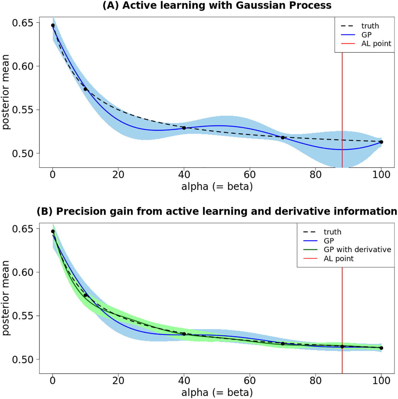
Estimation gains from adding grid point selected via active learning (AL) and derivative information (via AD). (A) Shows how active learning chooses the point with the maximum predictive variance from the Gaussian process (GP). (B) Shows the precision gain of the Gaussian process from adding the active learning point and the derivative information.
Figure 2B shows the true evolution of the posterior mean (dashed black line), the fitted Gaussian process without derivative (continuous blue line) and with derivative (continuous green line) after the active learning step. Incorporating derivative into Guassian process improves predictive performance in the mean-squared-error sense and reduces the predictive uncertainty, as measured by the 95 % predictive intervals (light green area versus light blue area). Comparing Figure 2A and B, we also observe that the uncertainty of the Gaussian process (without derivative) reduces considerably with the added point, and the fit has also improved.
Figure 2B shows that α
0 = β
0 ≈ 0 means a posterior mean approximately equal to 0.64, then the posterior mean decreases fast to stabilize after α
0 = β
0 ≈ 26 around 0.52. This aligns with the analytical expression of the posterior mean, as we have that
Example 2 (heteroskedasticity): Reduction in Evaluation Points. The second example illustrates sensitivity manifolds over prior mean and variance regions in a linear regression design with heteroskedasticity, and we consider a linear regression design with heteroskedasticity of the form
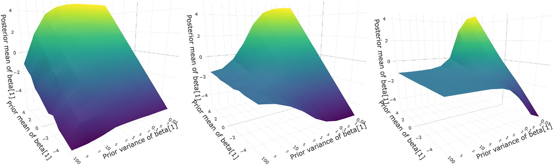
Sensitivity manifold graphing the posterior mean of β 1 over its prior mean and variance with increasing gamma parameter (ρ = 0.125 (left), ρ = 0.177 (middle) and ρ = 0.25 (right)).
In Figure 4, the first two panels show the reduction of grid points moving from a naive grid to a set of points chosen by the Gaussian process with active learning for estimating the sensitivity manifold. Instead of 187 grid points we now require only 64 points to reach an (uniform) uncertainty level of 0.18 over the surface. The last panel shows the reduction in uncertainty (the predictive variance is computed for 100 points randomly sampled from the surface, then the maximum is taken) in the sensitivity surface under the active learning based evaluation.
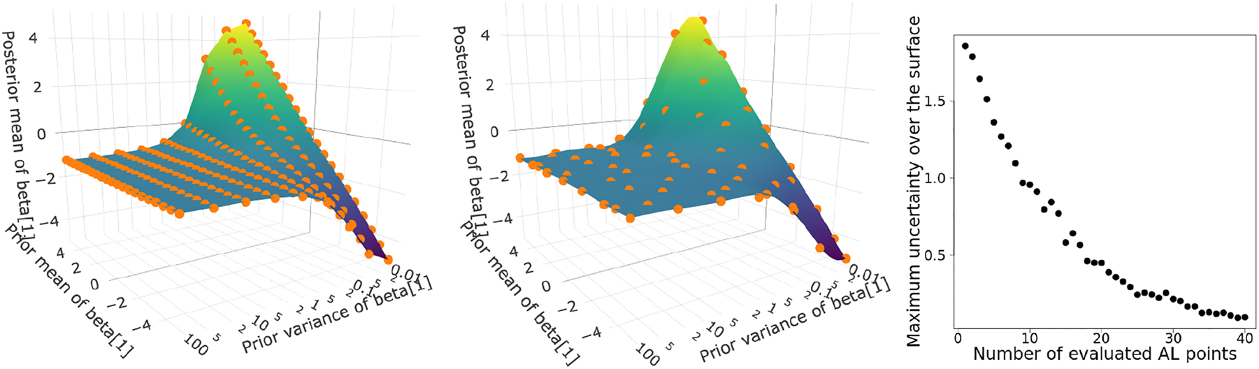
Sensitivity manifold β 1 over prior mean and variance with ρ = 0.25:11 × 17 = 187 points on an uniform grid (left, run-time: 61.5 s); 64 points using GP with active learning at 0.18 uncertainty (middle, run-time: 22.3 s); uncertainty of GP against the number of points evaluated after the initialisation (right).
3 Application: Prior Sensitivity of Posterior Price and Expenditure Elasticity Estimates
Reliable demand elasticity estimates are a key input for policy design, in many areas in economics, (public) health and beyond as they characterize key features of consumer behaviour. Our example considers the estimation of price and expenditure elasticities for food demand. Such estimates are used to examine the impact of food prices on food consumption and subsequent health consequences to assess policies targeting the growing problem of obesity and nutrition related health issues, and to investigate welfare consequences of rising food prices (Cornelsen et al. 2015; Gao 2012). Nonetheless, quality and robustness of empirical evidence on food demand elasticities remain an ongoing concern (Afshin et al. 2017; Nghiem et al. 2013). These are due to data limitations, but also estimation challenges relating to multivariate demand analysis under parameter constraints from economic theory (Baumeister and Hamilton 2019). Posterior inference on elasticities, functions of different demand parameters, requires the specification of a larger set of demand parameters and is likely to exhibit complex prior parameter dependencies that are potentially exacerbated by data limitations.
3.1 Inferential Framework for Food Demand Elasticities
Our empirical analysis is set within a widely-used multivariate demand system derived from micro-economic theory, efficiently estimated by standard MCMC methods, using data from an innovative Virtual Supermarket experiment with exogenous price variation. The so-called Linear Almost Ideal Demand System (LAIDS) is a popular framework to analyse nutrition choices and food policy interventions (Clements and Si 2016; Klonaris and Hallam 2003; Rickertsen, Kristofersson, and Lothe 2003; Tiffin and Arnoult 2010). It provides a multivariate demand analysis that captures a set of relevant food groups and choices. Importantly, the estimated substitution patterns are consistent across food groups (Briggs et al. 2013) and with underlying economic assumptions, such as the implied linear food Engel curves, supported by empirical evidence (Banks, Blundell, and Lewbel 1997). Bayesian MCMC methods offer an efficient and flexible approach to obtain inference on both elasticity point estimates and their precision within this demand framework for food shares that exhibits a number of economically motivated parameter restrictions (Bilgic and Yen 2014; Briggs et al. 2017; Kasteridis, Yen, and Fang 2011; Tiffin and Arnoult 2010).
3.1.1 Model Specification
Under LAIDS, originally proposed by Deaton and Muellbauer (1980), inference on price and expenditure elasticities are subject to restrictions arising from microeconomic theory. The Marshallian price elasticity (PE) of food group i with respect to food group j, ϵ ij and the expenditure elasticities for good i, η i under the LAIDS are:
where
where w
i
represents the spending shares on each food group
3.1.2 Prior-Posterior Inference for Virtual Supermarket Experiment
We focus on elasticity inference within a demand analysis of five main food groups (Fruits & Vegetables, Proteins, Starchy Foods, Drinks, Other), similar to the analysis in Clements and Si (2016) and Cornelsen et al. (2015). The anlaysis is based on a household sample from a Virtual Supermarket (VS) experiment (Waterlander et al. 2016) designed to address limitations in elasticity inference from insufficient and endogenous price variation in observational studies (Naghavi et al. 2017). The VS experiment contained 1412 unique food items positioned on supermarket shelves (about 75 % of the products in ‘real’ supermarkets) and was validated compared to actual shopping purchases in Waterlander et al. (2015). The sample contains 4258 completed shops where a household purchased from all main groups. In terms of budget shares, Fruits & Vegetables made up for 23 % of expenditure, Proteins (Meat and Dairy) 33 %, Starchy Foods 11 %, Non-Alcoholic Drinks 8 % and Other Foods (fats, oils, sweets, condiments) 25 % (see Jacobi et al. (2021) for more data details).
Main interest is on the posterior mean estimates of 16 price elasticities, ϵ = {ϵ ij : i, j = 1, 2, 3, 4}, and four expenditure elasticities, η = {η i : i = 1, 2, 3, 4} for the main food groups Fruits & Vegetables, Proteins, Starchy Foods and Non-alcoholic Drinks:[7]
where draws of the model parameters come from the posterior distribution of the model parameters, π( ϕ , Σ| y ) ∝ p( y | ϕ , Σ)π( ϕ , Σ).
Under the typical choice of conditionally conjugate priors in terms of independent Gaussian prior distributions on the vector of demand coefficients,
draws from the posteriors are generated via a standard two-step Gibbs sampler with a multivariate Normal update for the demand parameters and an Inverse Wishart update for the covariance parameter (see Appendix A.2 for the details on the Gibbs algorithm). There are 41 hyperparameters according to our specification, consisting of 18 locations and variances in the normal prior, and four elements in the scale matrix in the Inverse Wishart plus the degrees of freedom.
3.2 Sensitivity Analysis of Price Elasticities
In this section, we present the sensitivity analysis of the prior-posterior dependencies of the price elasticities. Different to previous illustrative examples, the application presents a more complex setting and exhibits larger prior parameter and output spaces. The analysis is structured around a series of questions that are relevant to practitioners, and we will use our manifold approach to address them. Part of the novelty comes from how our approach can give specific responses to key sensitivity-related questions that are not addressed by existing approaches. Beginning with the first basic set of questions, we are interested in
which input prior parameter has the biggest impact on the posterior output (i.e. price elasticity)?
which posterior outputs are the most sensitive to fluctuations in prior parameters?
how much would the posterior parameters change in response to small changes in a prior parameter?
These questions can be answered by studying the Jacobian of the posterior estimates, which we will compute from augmenting the MCMC estimation procedure with automatic differentiation (Jacobi, Zhu, and Joshi 2022). In our application the derivative information is initially computed to identify high sensitivity regions for the manifold construction, and hence is available for standard local analysis to complement the extended sensitivity assessment. This will be discussed in Section 3.2.1. The second set of questions are
what agreements/disagreements are there between the data and the expert opinion (expert-based priors)?
what is the decision turning point or boundary between two opinions (prior settings) that disagree with each other?
To answer these questions, we consider the scenario spectrum, which is the path connecting the two priors of interest in the prior parameter space. The scenario spectrum contains the “intermediate” priors between two priors, and we will build the posterior sensitivity manifold over this path. It will show how the two priors disagree with each other, and when a decision or a conclusion gets overturned as we switch from one prior to another in a continuous way. This will be discussed in Section 3.2.2. Finally, we investigate the question
how rapidly does the posterior statistics change across the region of interest?
This relates to the central question regarding the robustness of the analysis. The scenario spectrum provides a tool to quantify the robustness via visual and numerical measures that capture the variation of the posterior estimates as the input prior parameters change. We will use the Jacobian from the augmented MCMC procedure to explore the prior parameter space and identify the high sensitivity region, over which the posterior sensitivity manifold will be built. The manifold provides formal assessment of sensitivity analysis beyond the pointwise analysis, and this will be discussed in Section 3.2.3. The overview to our analysis is provided in Figure 5, and an illustration of how our approach goes beyond local assessment is provided in Figure 6.
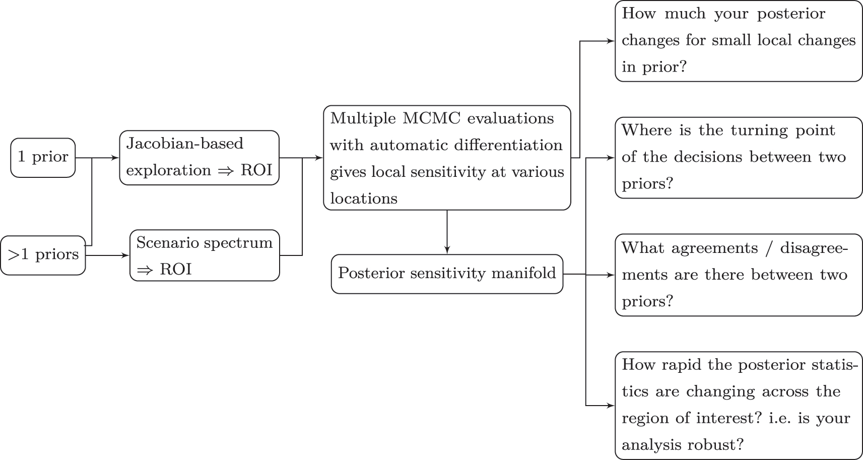
Sensitivity analysis with manifolds. The choice of priors includes the expert prior, the frequentist’s “prior”, and the non-informative prior. ROI stands for region of interest.
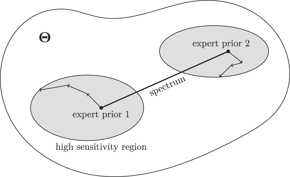
Illustration of the two strategies going beyond local assessments of prior parameters. The line connecting the two priors represents the prior “spectrum” which is the path connecting two set of prior parameters in the prior parameter space Θ. The grey areas are the high sensitivity regions discovered by the use of the Jacobian of the posterior estimates, depicted by the arrows. Manifolds are estimated over the spectrum and the high sensitivity regions.
As the departure point of our extended sensitivity analysis, Figure 7 presents the posterior estimates and frequentist estimates in the spirit of a standard scenario-type analysis. The posterior estimates are computed based on the expert prior, elicited based on expert advice and available PE estimates from previous observational studies (Jacobi et al. 2021). For comparison purposes, we also present the posterior estimates computed based on the non-informative prior. This prior will serve as the proxy prior corresponding to the frequentist estimate in some of the following analysis. As a technical note, the expert advice only provides estimates for the location parameters, but not the precision parameters. The precision parameters are solved by matching the coefficient of variations of the frequentist estimates at a particular ratio, and the ratio is set such that 50 % confidence is placed on the expert prior and 50 % of confidence is placed on the data. For the non-informative prior, the ratio is set such that 90 % confidence is placed on the data and 10 % confidence is placed on the expert prior. The details are provided in Appendix A.2, and the full table of the prior parameters and the posterior estimates are given in Appendix A.4.
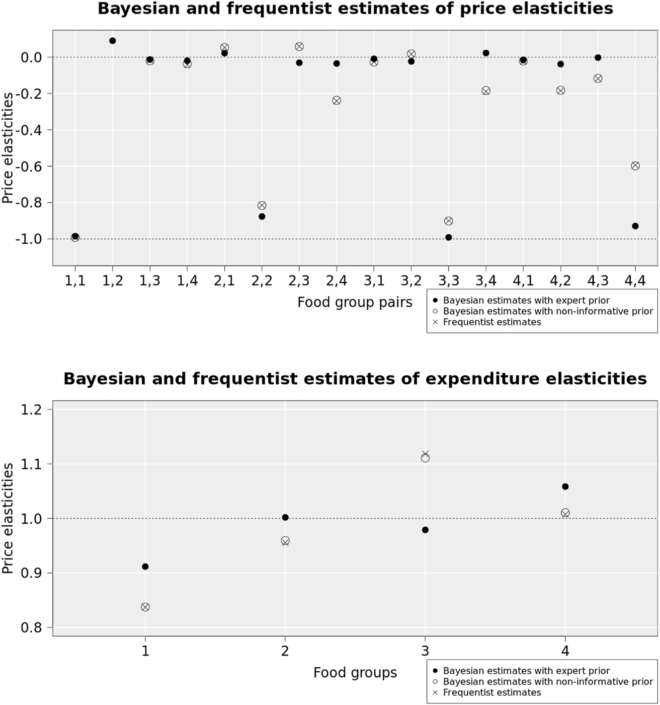
Bayesian estimates using the expert prior and Bayesian estimates using the non-informative prior and frequentist estimates of the price and expenditure elasticities.
3.2.1 Local Prior Parameter Dependence of Elasticity Estimates
We begin the sensitivity analysis locally at the expert prior by evaluating at the prior the Jacobian matrix of the posterior price elasticities with respect to the prior parameters. The partial derivatives in the Jacobian matrix provides valuable information about how the posterior output would respond to a small change in the prior input parameters. This helps us identify the most influential prior input parameter, as well as the most sensitive posterior price elasticity.
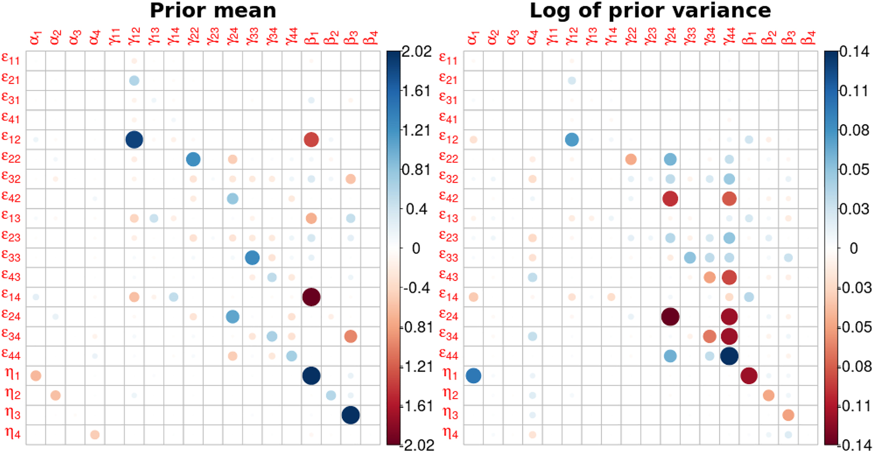
For computational efficiency and precision, the Jacobian matrix is computed based on the Gibbs IPA approach introduced in Jacobi, Zhu, and Joshi (2022) using automatic differentiation (AD) (Kwok, Zhu, and Jacobi 2020, 2022) that enables us to obtain unbiased derivative estimates alongside the MCMC estimation. The results are presented in Figure 8. The matrix entries are the sensitivities that represent how much the price and expenditure elasticities would respond to an instantaneous change in the prior specification. Each row reflects the partial derivative of a posterior elasticity estimate with respect to the prior mean or variance demand parameters, i.e. gradient information about the sensitivity manifold of a specific elasticity at a specific hyperparameters set. The dots represent non-zero partial derivatives of a particular elasticity with respect to a particular input with the magnitude indicated by size and colour.
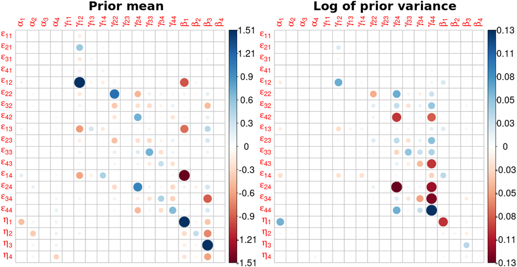
Jacobian matrix for price and expenditure elasticities with 50 % confidence on expert priors. The left graphs show the sensitivity with respect to the prior means; the positive part is capped at 1.51 to preserve the symmetry of the colour scale. The right graphs show the sensitivity with respect to the log of the prior variance; the positive part is capped at 0.13.
We discuss two key findings from the results. Firstly, not all prior parameters matter, and not all elasticity estimates are locally sensitive to changes in the prior parameters, as we observe from the sparseness of the Jacobian matrix. For the Jacobian matrix with respect to the prior mean of the prior parameters, the large sensitivities are observed only in the partial derivatives of ϵ 12 with respect to γ 12, ϵ 14 with respect to β 1, η 1 with respect to β 1 and η 3 with respect to β 3. For each of them, a ceteris paribus small unit variation in the input would change the posterior mean of the price elasticity by ≥1.51 units, for instance from ϵ 12 = 0.091 to ϵ 12 = 0.106 approximately given a 0.01 change in γ 12. Next, we can identify the most influential input parameter by finding which column of the Jacobian matrix has the largest column absolute sum (i.e. the column sum of the absolute values of the entries), as the sum aggregates the changes in all the price elasticities as the prior parameter of interest varies. The three most influential location parameters are the prior mean of γ 12, β 1 and β 3, and the three most influential precision parameters are the prior variance of γ 24, γ 34, and γ 44. Similarly, the row of the Jacobian matrix with the largest row absolute sum shows which price elasticity is the most sensitive. The three most sensitive price elasticities with respect to prior means are ϵ 12 ϵ 14 and η 1, and the three most sensitive price elasticities with respect to the prior variance are ϵ 24, ϵ 34, and ϵ 44.
Secondly, the Jacobian matrix reveals interesting patterns in the input and output parameters. For the prior mean of the input parameters, we know from equation (7) β i , i = 1, 2, 3, 4 contribute to the expenditure elasticity, but only from the Jacobian matrix we find out α i , i = 1, 2, 3, 4 also matter, although not that much. Regarding the price effect, while it is expected to see γ 12 affects ϵ 12 and likewise γ 22 affects ϵ 22, it is not known apriori that γ 11 and γ 13 have little local effect on any of the price elasticities. The Jacobian matrix also shows non-trivial interplay between the price effect and the price elasticity, as we see that γ 24 not only affects ϵ 24, but also ϵ 22, ϵ 44 in the opposite way, which can be confirmed by examining the reverse effect, i.e. the effect of γ 22 on ϵ 24. Regarding the expenditure effects, β 1 affects ϵ 12, ϵ 13, ϵ 14, η 1 as expected, but β 4 shows little effect on any of the elasticities, while β 3 shows effect on a wide range of elasticities. For the prior variance, we observe sensitivities are concentrated on the price effects γ 24, γ 33, γ 34, γ 44. Overall, the Jacobian matrix offers a thorough summary of the relationships between the input and output parameters, along with helpful empirical insights that theory alone may not provide.
3.2.2 Assessing Impacts of Prior Parameters with Scenario Spectrum
It is not uncommon in empirical studies to have more than one (expert) opinion or views, and it is instructive to understand how two opinions differ and how a decision may change as we switch from one expert opinion to another. As (expert) opinions are encoded via the prior specifications, it is possible to compare two (expert) opinions by comparing two prior specifications. To that end, we propose to construct a manifold over the scenario spectrum. A scenario spectrum is any path connecting two prior specifications in the prior parameter space that allows one to continuously vary from one prior specification to another.
The scenario spectrum is built around the observation that for any two sets of hyperparameters, it is possible to form a valid convex set of hyperparameters by linearly interpolating between them. This is based on the fact that both positivity of real numbers and positive semi-definiteness of real matrices are closed under the convex transform (e.g. linearly interpolating two covariance matrices gives a covariance matrix), so the interpolated hyperparameter would still be valid. These properties also generalise to multiple sets of hyperparameters. Mathematically, given some hyperparameters labelled by θ 1, θ 2, …, θ m , a scenario spectrum can be constructed as the convex set
When {w i , i = 1, 2, …, m} take value from the standard basis, i.e. all zeros except one entry with value 1, the scenario spectrum collapses back to the conventional scenario analysis. Hence, the scenario spectrum can be viewed as an extension of the scenario (and perturbation) analysis, which compares posterior inference across a few discrete points in the prior parameter space by rerunning the MCMC chains (An and Schorfheide 2007; Chib and Ergashev 2009; Roos et al. 2015). As the scenario spectrum fills in the gaps of the scenario analysis, it can be used to identify the points in the hyperparameter space where a policy decision is reversed, as well as the inconsistencies between the various prior specifications.
Taking the convex set is one way to build the scenario spectrum, but in our case, there is no need to do so because the way the expert prior is constructed naturally produces a scenario spectrum – we could simply vary the confidence in the expert prior. Assigning low and high confidence to expert location parameters is a useful strategy for generating two priors that present opposite ends of the scenario spectrum, and then varying the confidence in-between yields the entire spectrum.
In Figures 9 and 10, we show the manifold over the confidence in the expert prior information, ranging from 10 % (little confidence) to 90 % (high confidence). Note that the 50 % point is the expert prior used in our baseline analysis. It is observed that the non-informative prior recovers the frequentist estimates, whereas the posterior estimate reduces to the prior specification when high confidence is placed in the expert prior.
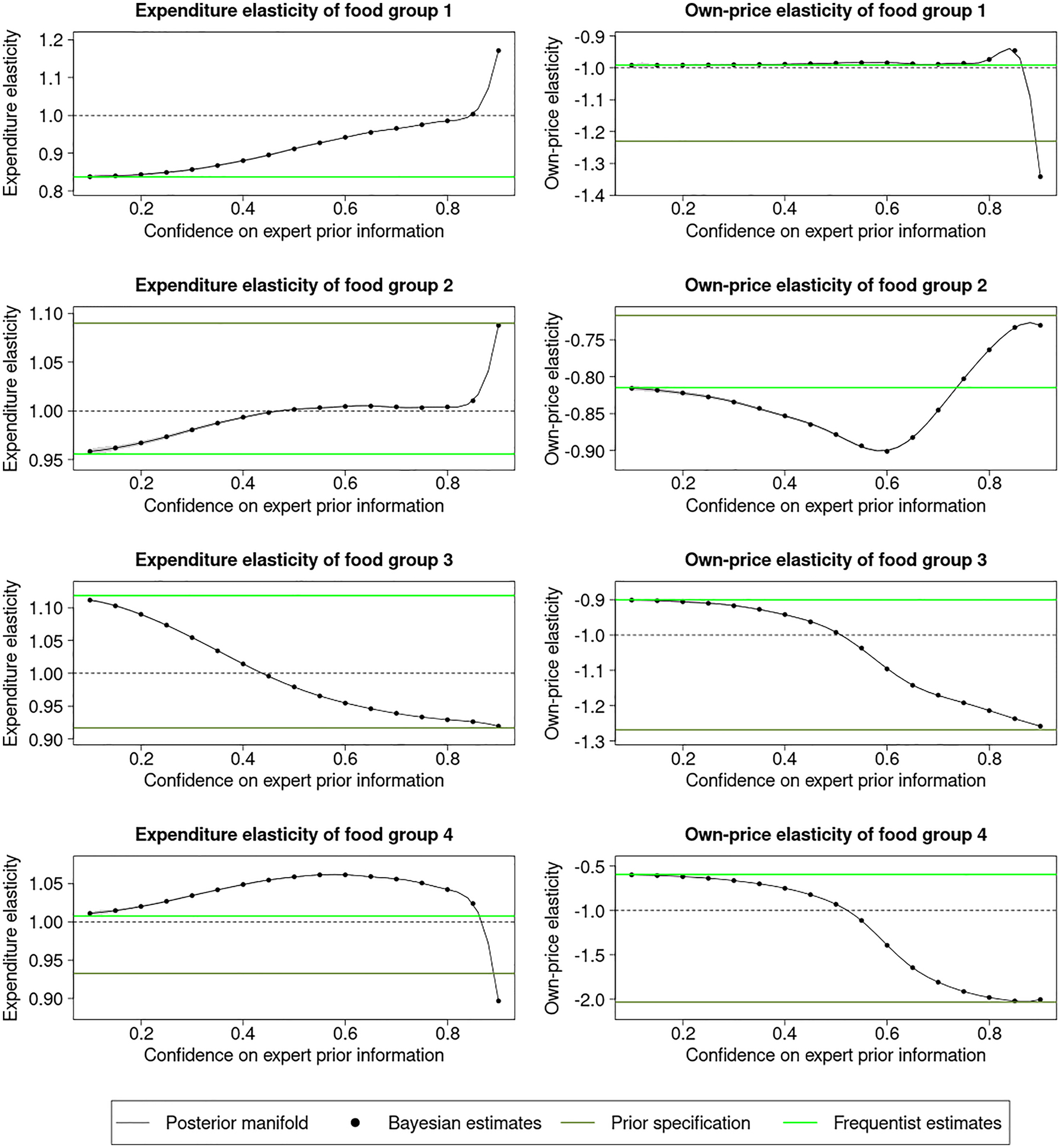
Manifold of own-price and expenditure elasticities over the scenario spectrum varying the confidence on the expert prior.
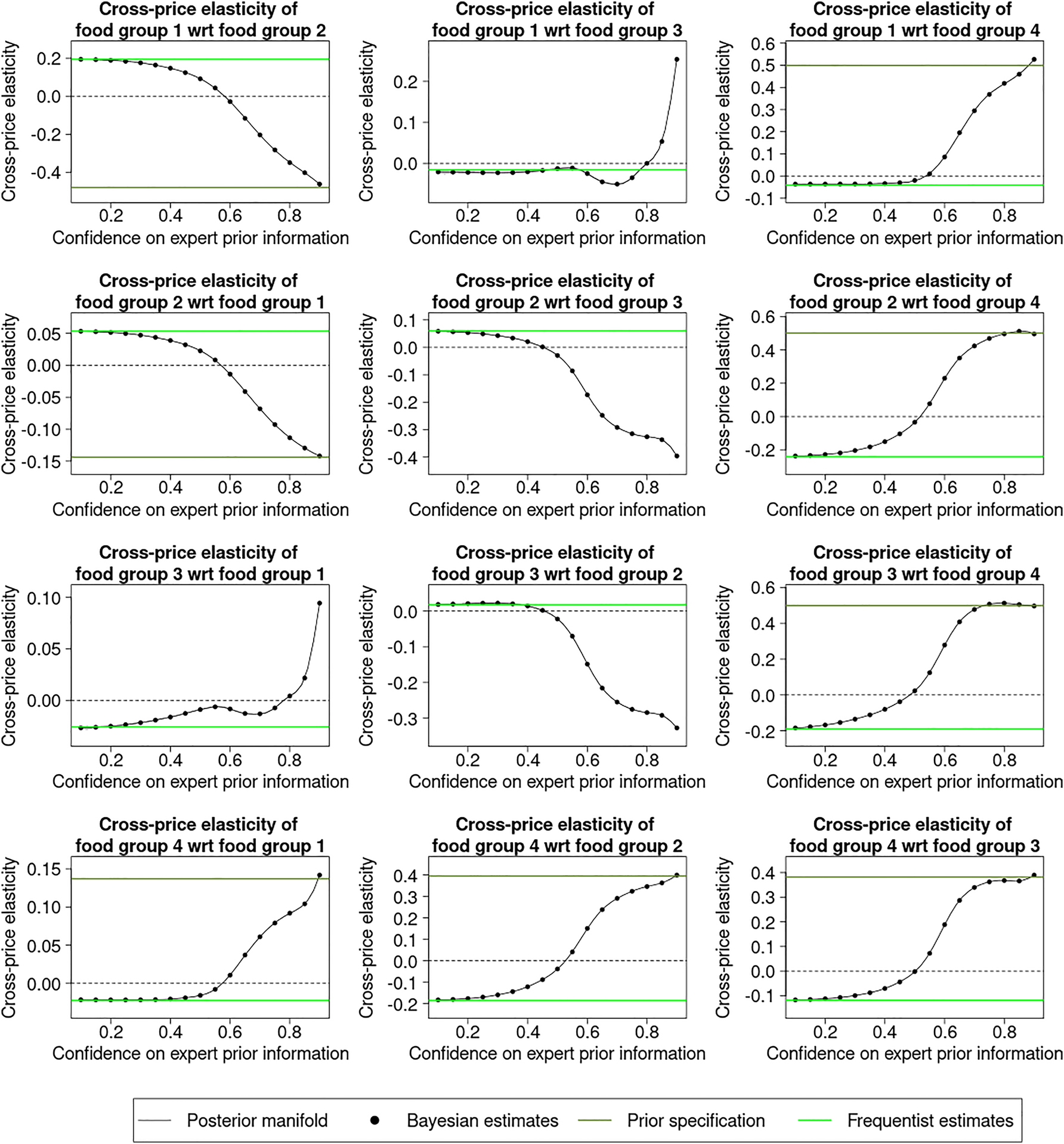
Manifold of cross-price elasticities over the scenario spectrum varying the confidence on the expert prior.
Interpreting the frequentist estimate as the estimates representing the data, we observe agreement between the data and the expert prior in the expenditure elasticities and own-price elasticities of food groups 1–4 with varying magnitudes of effects. For the expenditure elasticities of food groups 1, 2 and 4 and own-price elasticity of food group 1, large changes are observed near the end of the spectrum where extremely high confidence is placed in the expert prior information, indicating that the expert prior specification is excessive relative to the data. For the cross-price elasticities, denoting the cross-price elasticity of food group i with respect to food group j by ϵ ij , we observe minor disagreement between the data and the expert prior specification in ϵ 13, ϵ 21 and ϵ 31 and major disagreement, i.e. the elasticities at two ends lie on different sides of the reference line with large gaps in-between, in ϵ 12, ϵ 14, ϵ 23, ϵ 24, ϵ 32, ϵ 34, ϵ 41, ϵ 42 and ϵ 43.
We observe the turning point where the cross-price elasticities cross the reference line at around 0.5–0.6 (see for example ϵ 12, ϵ 41 and ϵ 34). Note that 0.6 (or 60 %) confidence on the expert and 0.4 (or 40 %) confidence on the data indicate that the variance of the expert prior parameter is approximately two-thirds the variance of the frequentist estimates. If the experts were confident about the location parameters and imposed tight variances on them, then the Bayesian estimates would reflect this and lean towards the expert specifications.
In practice, it is recommended to build the manifold over the confidence range of 0.1–0.5, where 0.5 corresponds to equal confidence on the expert prior and the data, since a confidence mix of 90 % on expert and 10 % on data is implausible. We did this to emphasise the contrast between the prior and the data and to reinforce a point seen in many of the classic examples in Bayesian analysis, namely that the posterior estimates interpolate between the frequentist estimates and the expert prior information. In simple cases where analytic formulae are available, interpolation can be linear, as seen in Example 1 of Section 2.4, whereas in complex cases where MCMC inference is required, interpolation can be nonlinear, as shown by the presented results.
3.2.3 Assessing Impacts of Prior Parameters with High Sensitivity Region
We now turn to studying how rapidly the posterior statistics change across the region of interest, which provides a mathematical response to the question “is your analysis robust?”. We begin by discussing how to identify a high sensitivity region, which serves as a good starting point when the region of interest is unknown at the outset, and then we measure and visualise the sensitivity using the posterior sensitivity manifold built on the region.
To identify the high sensitivity region, we start with an expert prior and perform the AD-augmented MCMC inference to get the Jacobian matrix. Using the Jacobian, we move the expert prior point towards the steepest ascent in the prior parameter space and re-evaluate; iterating this step N 0 times yields an ascent trajectory. Then we restart from the beginning, but this time we move the expert prior point towards the direction of the steepest descent and obtain the descent trajectory. At the original expert prior, the trajectory of descent meets the trajectory of ascent. Overall, we explored the prior parameter space by taking the steepest paths and attempting to cause the greatest change in the posterior output (i.e. the price elasticities). The high sensitivity region is defined as the minimum bounding box of the full trajectory. It contains the starting expert prior, all the evaluated points on the full trajectory and all scenario spectrum that are built as the convex set of the evaluated points.
The comprehensiveness of the high sensitivity region comes at a cost that it is computationally more expensive to build a manifold on the high sensitivity region, due to the curse of dimensionality. While active learning can help to alleviate the problem, how well it works is determined by the complexity of the posterior sensitivity manifold; the simpler the manifold, the better. In practice, it is advised to use the Jacobian matrices computed along the trajectory to inform what input and output parameters to investigate. This builds on the sparseness of the Jacobian matrices and reduces the high dimensions down to only the relevant ones, keeping the analysis tractable.
We perform our analysis for the 20 expected values of the price elasticities and four expenditure elasticities. The gradient exploration is based on N 0 = 5 number of steps.[8] We average over the 2N 0 + 1 = 11 Jacobian matrices to produce the aggregate Jacobian, shown in Figure 11. We can see that as in the case of the local analysis, the aggregate Jacobian helps us identify the most influential inputs and most sensitive outputs.
The aggregate Jacobian of the price elasticities, averaged over the Jacobian matrices from the gradient steps.
Figure 11 indicates that the most influential inputs regarding the prior mean are associated with γ 12, γ 22, γ 24, β 1 and β 3, whereas the most influential inputs associated with the prior covariance matrix of the location parameters are Var(α 4), Var(γ 24), Var(γ 34), Var(γ 44) and Var(β 1). On the other hand, the most sensitive elasticities are ϵ 12, ϵ 14, ϵ 34, η 1 and η 3. For instance, a ceteris paribus 0.1 change in the prior mean of β 1 would cause a change in ϵ 14 approximately equal to −0.2.
As an auxiliary information, it is useful to report the max norms of the Jacobian matrices, which corresponds to the change of the most sensitive entry with respect to its most influential input. This provides a one-number summary for each of the Jacobian matrices. In the order of [−5, −4, −3, −2, −1, 0, 1, 2, 3, 4, 5] steps, the max norms of the Jacobian matrices along the trajectory are [11.99, 11.99, 11.97, 11.99, 11.96, 4.05, 7.71, 6.57, 5.62, 6.85, 5.79]. Observe the asymmetry of the max norms along the descent and ascent trajectories. It indicates that price and expenditure elasticities respond differently to increment and decrement in the prior parameters.
Once the gradient trajectory is traced out, we identify the minimum bounding box of the trajectory as the region of high sensitivity. Table 1 reports the prior input dimensions and the associated bounds of the most influential prior demand parameters according to Figure 11. Using Equation 3.1.1 where
Influential prior parameter dimensions from 5-step gradient procedure around the expert prior. Reported are the upper and lower bounds of the prior mean and variance settings. Variance hyperparameters are in log-scale. Results given for most influential prior inputs, i.e. yielding largest change in posterior elasticity inference in the most sensitive elasticity outputs.
| Range of influential location and variance input dimensions | |||||||
|---|---|---|---|---|---|---|---|
| Location settings | (log) Variance settings | ||||||
| Coeff. | Mean LB | Expert | Mean UB | Coeff. | Var LB | Var | Var UB |
| γ 12 | −0.099 | −0.032 | 0.035 | α 4 | −8.599 | −8.317 | −8.023 |
| γ 22 | 0.000 | 0.071 | 0.142 | γ 24 | −9.920 | −9.881 | −9.842 |
| γ 24 | 0.083 | 0.124 | 0.165 | γ 34 | −9.165 | −9.101 | −9.037 |
| β 1 | −0.005 | 0.017 | 0.039 | γ 44 | −9.108 | −9.078 | −9.049 |
| β 3 | −0.288 | −0.021 | 0.246 | β 1 | −12.068 | −12.047 | −12.014 |
Next, we will construct the manifold over the region of high sensitivity. Note that the total of 36 prior mean and variance parameters makes estimating the manifold challenging. Because, in order to specify a bounding box, two endpoints per dimension would be required, and there would be approximately 236 ≈ 68 billion vertices. But as we saw in the analysis of the aggregate Jacobian matrix, only a few inputs and outputs are significant, so we will focus on these parameters. They are the prior mean of γ 12, γ 22, γ 24, β 1, β 3 for the most influential input and the price elasticities of ϵ 12, ϵ 14, ϵ 34, η 1, η 3 for the most sensitive output. The remaining prior parameters are set at the expert prior levels. Once the five dimensional manifold embedded in the 36 dimensional space is estimated, we compute the maximum variation range using Equation (2) for each of the sensitive elasticities. The results are presented in Table 2.These numerical measures indicates the robustness of the analysis. We observe that the cross-price elasticity ϵ 12, ϵ 14 are stable despite the change of sign in the ϵ 12. The cross-price elasticity ϵ 34 and the expenditure elasticities η 1 and η 3 have large variations, with ϵ 34 switching from complementary effect to substitute effect and η 3 varying from small increase of demand to large increase of demand in response to an increase in expenditure.
Bounds (min and max) of sensitivity manifolds of top five most sensitive price and expenditure elasticities over the 5-dimensional high sensitivity region
| Summary of high sensitivity region manifolds | |||
|---|---|---|---|
| Price elasticities | Min | Max | Variation |
| ϵ 12 | −0.02 | 0.06 | 0.09 |
| ϵ 14 | −0.03 | −0.00 | 0.03 |
| ϵ 34 | −0.19 | 0.37 | 0.56 |
| η 1 | 0.71 | 1.19 | 0.48 |
| η 3 | 0.18 | 1.64 | 1.47 |
Finally, we present visualisations of the sensitivity manifold to highlight its geometric aspects. A limitation of the ad hoc scenario analysis, as well as the maximum variation range sensitivity measure, is that they cannot uncover relationships between variables at a more granular level. We saw earlier that scenario spectrum can help us discover the inflection points where decisions are overturned, we will show how three-dimensional subspace plots can show the interplay between the posterior output and the different prior input parameters. We generate the plots based on the most influential input parameters and most sensitive output shown in Tables 1 and 2, and Figure 11. In particular, we perform the sensitivity analysis for the posterior mean of the cross price elasticity between Starchy Foods and non-alcoholic drinks
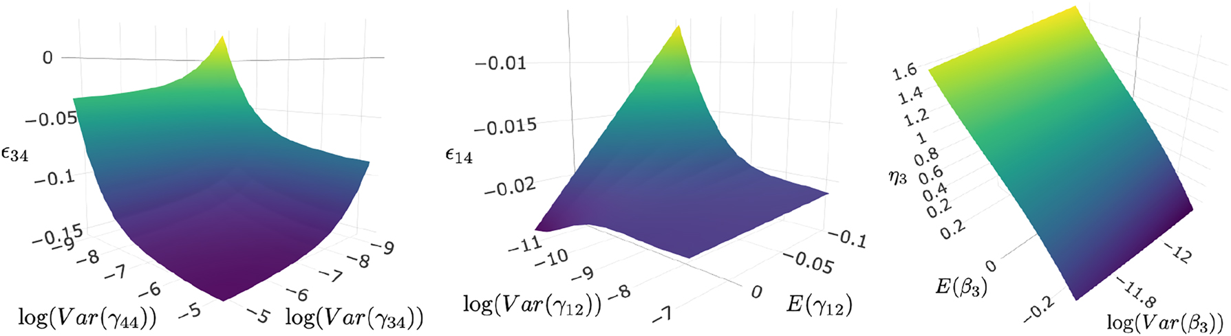
Cross-price elasticity surface of food group 3 and 4 (left), cross-price elasticity surface of food group 1 and 4 (middle), and expenditure elasticity of food group 3 (right). Variances are displayed in log-scale.
The three plots in Figure 12 show different aspects of the posterior inference. Starting on the right, we can see that the expenditure elasticity of food group 3 remains positive even when the prior expenditure effect changes sign from −0.2 to 0.2, and the 0.4 variation in the expenditure effect translates into the magnified 1.4 variation in the elasticity. The magnitude of the elasticity is determined largely by the prior effect, as we observe a clear linear relationship between the prior effect and the posterior elasticity. The changes in the tight variance only affect the elasticity slightly. In the middle plot of the cross-price elasticity of the first and fourth food groups, we observed a peculiar non-negligible effect from prior mean of γ 12, a term that does not appear in Equation (7). This shows that while γ 12 does not theoretically relate to ϵ 14, its prior specification has a competing effect with γ 14 during estimation. At low variance, the variation in the prior mean maps linearly to the variation of the elasticity, and as the variance increases, the prior mean loses its effect. In contrast to the right plot, the size of the prior variance determines where the elasticity will be given a fixed prior mean.
In the left plot, we show the cross-price elasticity of the third and fourth food groups against two prior variances in log-scale. The upper bounds of the variances are expanded, in part to enhance the visualisation and in part because the ranges were so narrow that there was ample computational power remaining. We observe non-linear relationship between each of the prior variance and the elasticity, with γ 44 having a larger effect than γ 34. If we were to slice the surface with a horizontal plane, we would find the level set, i.e. the set in which elasticity has a constant value, which reveals the relationship between the two variances. Specifically, it describes how increased confidence in one variable and decreased confidence in another can cancel each other out and leave the results unchanged. The interdependence demonstrates that the specification of prior variances is a complex endeavour. Finally, we observe as both prior variances increase, the elasticity surface becomes flat, and the value stabilises.
As a closing remark, we saw that the interaction between the prior mean and the prior variance specification can be subtle. When the prior mean specification differs greatly from the sample information and a tight variance is imposed, the posterior inference can be highly sensitive. Other factors, however, can come into play. For example, when the likelihood function becomes flat, as in the case of the normal density with a very high variance, or when the prior distribution is concentrated on the likelihood’s tails, the sensitivity can be further magnified (Ramírez-Hassan and Pericchi 2018).
4 Conclusions
The introduced concept of sensitivity manifolds over hyperparameter regions and the computational approach to estimate manifold-based sensitivity measures for MCMC inference links popular pointwise and local perspectives. Importantly, by doing so it extends assessment of prior parameter dependence beyond their limited scope to answer questions regarding the prior parameter sensitivity (robustness) that arise in many practical problems of Bayesian MCMC inference. Firstly, researchers typically consider values within a feasible or sensible region of the hyperparameter(s), often informed by previous studies or theoretical considerations, rather than a set of possible discrete points in the hyperparameter space. Secondly, researchers are often interested not just in whether an analysis is robust to misspecification – in fact, it is well understood that assumptions matter a great deal in practical problems, and they are not always robust – but also how the analysis would change when the prior specification changes.[9] Further, understanding how the posterior analysis depends on the prior parameters helps researchers set sensible prior parameters which remains a challenging task due to well-known issues such as model complexity, cost of prior elicitation, flat priors and identification issues.
The approach acknowledges that reliable specification of prior information remains difficult and that researchers often consider a range of potentially reasonable prior parameter settings for each parameter. We hope that the proposed methods contribute to the appeal of Bayesian inference for applied analysis as a well-designed prior robustness analysis can further increase transparency and confidence of policy makers in Bayesian inference. The methods also offer a tool to better understand the impact of common or default priors widely used in many applications, which is important as the extent to which prior assumptions influence posterior inference will vary across applications and data sets.
Acknowledgement
We are grateful to seminar participants at ESOBE (St Andrews), ANZESG (Melbourne), NBER-NSF (Saint Louis, online), IAAE (online), Monash University (Melbourne), Melboure Bayesian Econometrics workshop and University of Linz.
-
Research funding: LJ acknowledges funding from the Australia Research Council (https://doi.org/10.13039/501100000923) through FT170100124. CFK acknowledges funding from the Australia Research Council (https://doi.org/10.13039/501100000923) through DP180102538. NN acknowledges funding from the Health Research Council of New Zealand (https://doi.org/10.13039/501100001505) through grant 16/443.
A.1 Gaussian Processes
A Gaussian process (GP) is a collection of random variables, any finite of which have a joint Gaussian distribution (Rasmussen and Williams 2006). It is specified as
where m( θ ): R p → R is the mean function and k( θ , θ′): R p × R p → R is the kernel/covariance function and θ and θ ′ are two input values. It can handle a wide range of data generating processes, adapt to data, capture uncertainty well and it is easy to implement.
Given some function values s (n × 1) evaluated at the coordinates Θ n (n × p), the zero mean function and a kernel function k ψ (⋅, ⋅), the estimation of the kernel parameters ψ proceeds as follows. Under the model assumption, we have
where K ψ (Θ n , Θ n ) is the n × n matrix with the (i, j) entry = k ψ ( θ i*, θ j*), θ i* denotes the i-th row of the matrix Θ n . Writing K ψ (Θ n , Θ n ) as K ψ and denoting the determinant function by |⋅|, the log-likelihood is given by
The kernel parameters ψ can be found using Maximum Likelihood Estimation (MLE). Note that the computational complexity is O(n 3) due to the inversion of matrix needed to evaluate the likelihood. But this will not pose a problem as n is small in our application. If needed, approximate methods are also available to reduce the computational complexity from O(n 3) to O(n); interested readers are referred to Gardner et al. (2018), Pleiss et al. (2018) and Wilson and Nickisch (2015).
Given new evaluation points
The conditional distribution is given by
where K ij is the (i, j)-th block entry in (8), and the conditional mean is used as the prediction.
To add derivative information for improving precision in the inferential process, the point of departure is that the derivative of a GP is also a GP, and we have
where
A.2 Real Data Analysis: MCMC Inference
Given the standard assumption, ϵ (h) ∼ N 5(0, Σ), the resulting LAIDS model can then be rewritten into the Seemingly Unrelated Regression (SUR) model so that the likelihood, without loss of generality, is given by
where
Table 7 shows the default elicited prior hyperparameters for the location parameters in the LAIDS model. That is, our point of departure for θ 0 are the parameters in this table, and R 0 = I 4 and ρ 0 = 4, which we set in order to be non-informative regarding the hyperparameters of the covariance matrix.
The prior variances of the demand parameters are specified in terms of a prior weight ratio r:
where “coef est
i
” and “se est
i
” are the frequentist estimates of the coefficients and their standard errors. Observe that
Without loss of generality, α i , i = 1, …, 4, γ ij , i ≤ j, j = 1, …, 4 and β i , i = 1, …, 4 are chosen as the free parameters.
The data is modelled by the SUR model
Initialise Σ 0, set g = 1.
Draw ϕ (g) from
Draw
Set g = g + 1. If the maximum number of iteration is not reached, go back to 2.
A.3 Supplementary Analysis
A.3.1 Gaussian Process versus Neural Network
It is instructive to compare the performance of Gaussian Process with artificial Neural Network (NN) on sparse grid points.
We considered the Bayesian linear regression model, same as Example 2 in Section 2.4 but without heteroskedasticity, y ∼ N(Xβ
, σ
2
I),
The NN is fitted using the nnet package in R. We considered fully connected networks with 1 hidden layer, of size from 2 to 10, each with 100 random initialisations. We pick the best model for NN using the testing dataset to favour it more.
Comparing the predictions with the ground truth, we get a mean squared error of 4.42 × 10⁻⁵ from GP and 1.346958 from NN. The drastic difference here is due to that NN did not learn properly in some of the dimensions. The mean squared errors by dimensions are provided in Table 3.
Dimension-by-dimension comparison of GP and NN on a fixed grid. Numbers are mean squared errors.
| k-th dimension | 1 | 2 | 3 | 4 | 5 |
|---|---|---|---|---|---|
| GP | 5.40 × 10⁻⁵ | 8.48 × 10⁻⁵ | 4.07 × 10⁻⁵ | 2.29 × 10⁻⁵ | 1.87 × 10⁻⁵ |
| NN | 1.36 | 0.64 × 10⁻⁵ | 0.012 | 5.36 | 0.47 × 10⁻⁵ |
NN failed to learn for dimensions 1 and 4, while for dimensions 2 and 5, it did outperform GP. The result confirms a well-accepted empirical observation that GP generally does better than NN in data-poor regime and the other way around in data-rich regime.
A.3.2 Gaussian Process with Active Learning in Higher Dimension
It is helpful to investigate if Gaussian Process with active learning can handle larger hyperparameter dimensions.
We consider the same linear regression model with conditional prior distributions as the last section, i.e. y ∼ N(Xβ
, σ
2
I),
We conducted the simulation with increasing number of dimensions (p = 5, 10, 20, 40) and report the mean squared error (MSE) comparing with the analytical formula and the computing time. The experiment was conducted using eight cores with 40 GB RAM on an HPC cluster. The result is provided in Table 4.The result supports that our method can handle larger hyperparameters dimension with reasonable precision and computing time.
Accuracy and computing time of the sensitivity manifolds.
| #Dimensions | p = 5 | p = 10 | p = 20 | p = 40 |
|---|---|---|---|---|
| MSE | 0.15 × 10⁻⁴ | 0.22 × 10⁻⁴ | 1.40 × 10⁻⁴ | 4.02 × 10⁻⁴ |
| Time | 46.00 s | 331.98 s | 1537.57 s | 6043.86 s |
A.3.3 Gaussian Process with and without Derivatives
It is informative to explore the trade off between the use of derivatives and simply increasing the number of grid points without derivatives.
Considering the trade-off between derivatives and grid points in terms of finite-differencing, in a p-dimensional space, p + 1 evaluations are required to find all the partial derivatives at a point using finite differencing. So the information contained in a derivative may be considered to correspond to p grid points in a small neighbourhood. The correspondence is exact in the simple case when the sensitivity manifold is a hyperplane. In general, the “shape” of the sensitivity manifold determines the trade-off between derivatives and grid points, and it should be studied on a case-by-case basis.
We conducted an experiment for when p = 10, 20, 30. In each setting, we first fit a GP with derivatives and then a GP (without derivatives) with increasing number of grid size and observe when its accuracy becomes as good as the GP with derivatives, or if it fails to reach the accuracy within the computing budget of GP with derivatives. The result is summarised in Table 5.
Trade-off between the use of derivatives and increasing the number of grid points without derivatives for p = 10, 20, 30. Mean squared errors (MSE) are computed by comparing with the analytical formula.
| #Evaluation points | 100 | 500 | 1000 | 2000 | 4000 | 100 + AD |
|---|---|---|---|---|---|---|
| p = 10 | ||||||
| MSE (×10−7) | 1345.84 | 76.54 | 21.21 | 5.75 | 1.7 | 3.37 |
| Time | 6.44 s | 49.95 s | 148.58 s | 453.16 s | 1412.16 s | 373.52 s |
| p = 20 | ||||||
| MSE (×10−7) | 3295.89 | 630.06 | 196.41 | 48.5 | 15.05 | 5.13 |
| Time | 12.03 s | 107.56 s | 329.21 s | 919.13 s | 3457.73 s | 1051.83 s |
| p = 30 | ||||||
| MSE (×10−7) | 5169.67 | 1861.54 | 743.16 | 225.23 | 72.36 | 186.62 |
| Time | 22.46 s | 209.96 s | 619.68 s | 2359.28 s | 7372.63 s | 2730.37 s |
For p = 10, GP (without derivative) caught up with GP with derivatives (100 grid points) in accuracy when 4000 grid points are used. The MSE of GP is about half of the MSE of GP with derivative, but the time taken to reach that accuracy is three to four times more.
For p = 20, GP did not reach the accuracy of GP with derivative in all the cases considered. With 4000 evaluation points, GP reached a MSE that was about three times the MSE of GP with derivatives, and it also took more time to complete.
For p = 30, like the first case, it took 4000 points for GP to reach the performance of GP with derivatives, with half the MSE and about three times the computing budget.
The results show that GP with derivative is generally more accurate given the same computing budget. However, if high precision is not required, then evaluating GP with more points (but not many more) may be more efficient. Since computing the derivatives incur some overhead cost, GP with derivative is more efficient only when the dimension is higher or a higher precision is sought.
A.4 Supplementary Tables and Figures
Prior parameters of the expert prior and the non-informative prior.
| Expert prior | Zero prior | |||
|---|---|---|---|---|
| Prior mean | Prior variance (×10−4) | Prior mean | Prior variance (×10−2) | |
| α 1 | 0.25 | 2.65 | 0.00 | 2.14 |
| α 2 | 0.25 | 2.78 | 0.00 | 2.25 |
| α 3 | 0.25 | 25.37 | 0.00 | 20.55 |
| α 4 | 0.25 | 2.44 | 0.00 | 1.98 |
| γ 11 | −0.02 | 16.15 | 0.00 | 13.08 |
| γ 12 | −0.03 | 0.13 | 0.00 | 0.11 |
| γ 13 | 0.03 | 0.86 | 0.00 | 0.70 |
| γ 14 | 0.04 | 0.54 | 0.00 | 0.44 |
| γ 22 | 0.07 | 0.88 | 0.00 | 0.71 |
| γ 23 | −0.11 | 14.77 | 0.00 | 11.96 |
| γ 24 | 0.12 | 0.51 | 0.00 | 0.41 |
| γ 33 | −0.07 | 1.23 | 0.00 | 0.99 |
| γ 34 | 0.12 | 1.12 | 0.00 | 0.90 |
| γ 44 | −0.34 | 1.14 | 0.00 | 0.92 |
| β 1 | 0.02 | 0.06 | 0.00 | 0.05 |
| β 2 | 0.02 | 0.60 | 0.00 | 0.48 |
| β 3 | −0.02 | 0.07 | 0.00 | 0.05 |
| β 4 | −0.02 | 11.65 | 0.00 | 9.44 |
Bayesian and frequentist estimates of price and expenditure elasticities.
| Bayesian estimates | Frequentist estimates | |
|---|---|---|
| Price elasticities | ||
| ϵ 11 | −0.99 | −0.99 |
| ϵ 12 | 0.02 | 0.05 |
| ϵ 13 | −0.01 | −0.03 |
| ϵ 14 | −0.02 | −0.02 |
| ϵ 21 | 0.09 | 0.19 |
| ϵ 22 | −0.88 | −0.81 |
| ϵ 23 | −0.02 | 0.02 |
| ϵ 24 | −0.04 | −0.18 |
| ϵ 31 | −0.01 | −0.02 |
| ϵ 32 | −0.03 | 0.06 |
| ϵ 33 | −0.99 | −0.9 |
| ϵ 34 | 0.00 | −0.12 |
| ϵ 41 | −0.02 | −0.04 |
| ϵ 42 | −0.03 | −0.24 |
| ϵ 43 | 0.02 | −0.19 |
| ϵ 44 | −0.93 | −0.59 |
| Expenditure elasticities | ||
| η 1 | 0.91 | 0.84 |
| η 2 | 1.00 | 0.96 |
| η 3 | 0.98 | 1.12 |
| η 4 | 1.06 | 1.01 |
References
Afshin, A., J. L. Penalvo, L. Del Gobbo, J. Silva, M. Michaelson, M. O’Flaherty, S. Capewell, D. Spiegelman, G. Danaei, and D. Mozaffarian. 2017. “The Prospective Impact of Food Pricing on Improving Dietary Consumption: A Systematic Review and Meta-Analysis.” PLoS One 12 (3): e0172277. https://doi.org/10.1371/journal.pone.0172277.Search in Google Scholar PubMed PubMed Central
Amir-Ahmadi, P., C. Matthes, and M.-C. Wang. 2020. “Choosing Prior Hyperparameters: With Applications to Time-Varying Parameter Models.” Journal of Business & Economic Statistics 38 (1): 124–36. https://doi.org/10.1080/07350015.2018.1459302.Search in Google Scholar
An, S., and F. Schorfheide. 2007. “Bayesian Analysis of Dsge Models.” Econometric Reviews 26 (2-4): 113–72. https://doi.org/10.1080/07474930701220071.Search in Google Scholar
Banks, J., R. Blundell, and A. Lewbel. 1997. “Quadratic Engel Curves and Consumer Demand.” The Review of Economics and Statistics 79 (4): 527–39. https://doi.org/10.1162/003465397557015.Search in Google Scholar
Basu, S., S. R. Jammalamadaka, and W. Liu. 1996. “Local Posterior Robustness with Parametric Priors: Maximum and Average Sensitivity.” In Maximum Entropy and Bayesian Methods, 97–106. Dordrecht: Springer.10.1007/978-94-015-8729-7_6Search in Google Scholar
Baumeister, C., and J. D. Hamilton. 2019. “Structural Interpretation of Vector Autoregressions with Incomplete Identification: Revisiting the Role of Oil Supply and Demand Shocks.” American Economic Review 109 (5): 1873–910. https://doi.org/10.1257/aer.20151569.Search in Google Scholar
Berger, J. O. 1985. Statistical Decision Theory and Bayesian Analysis. New York: Springer Science & Business Media.10.1007/978-1-4757-4286-2Search in Google Scholar
Berger, J. O. 1990. “Robust Bayesian Analysis: Sensitivity to the Prior.” Journal of Statistical Planning and Inference 25 (3): 303–28. https://doi.org/10.1016/0378-3758(90)90079-a.Search in Google Scholar
Berger, J. O., E. Moreno, L. R. Pericchi, M. J. Bayarri, J. M. Bernardo, J. A. Cano, J. De la Horra, et al.. 1994. “An Overview of Robust Bayesian Analysis.” Test 3 (1): 5–124. https://doi.org/10.1007/bf02562676.Search in Google Scholar
Berger, J. O., D. R. Insua, and F. Ruggeri. 2000. “Bayesian Robustness.” In Robust Bayesian Analysis, 1–32. New York: Springer.10.1007/978-1-4612-1306-2_1Search in Google Scholar
Bhatia, K., Y.-A. Ma, A. D. Dragan, P. L. Bartlett, and M. I. Jordan. 2023. “Bayesian Robustness: A Nonasymptotic Viewpoint.” Journal of the American Statistical Association (15): 1–12, https://doi.org/10.1080/01621459.2023.2174121.Search in Google Scholar
Bilgic, A., and S. T. Yen. 2014. “Demand for Meat and Dairy Products by Turkish Households: A Bayesian Censored System Approach.” Agricultural Economics 45 (2): 117–27. https://doi.org/10.1111/agec.12019.Search in Google Scholar
Branson, Z., M. Rischard, L. Bornn, and L. W. Miratrix. 2019. “A Nonparametric Bayesian Methodology for Regression Discontinuity Designs.” Journal of Statistical Planning and Inference 202: 14–30. https://doi.org/10.1016/j.jspi.2019.01.003.Search in Google Scholar
Briggs, A. D., A. Kehlbacher, R. Tiffin, T. Garnett, M. Rayner, and P. Scarborough. 2013. “Assessing the Impact on Chronic Disease of Incorporating the Societal Cost of Greenhouse Gases into the Price of Food: An Econometric and Comparative Risk Assessment Modelling Study.” BMJ Open 3: 10, https://doi.org/10.1136/bmjopen-2013-003543.Search in Google Scholar PubMed PubMed Central
Briggs, A. D., O. T. Mytton, A. Kehlbacher, R. Tiffin, A. Elhussein, M. Rayner, S. A. Jebb, T. Blakely, and P. Scarborough. 2017. “Health Impact Assessment of the UK Soft Drinks Industry Levy: A Comparative Risk Assessment Modelling Study.” The Lancet Public Health 2 (1): e15–22. https://doi.org/10.1016/s2468-2667(16)30037-8.Search in Google Scholar PubMed PubMed Central
Chan, J. C., L. Jacobi, and D. Zhu. 2019. “How Sensitive Are Var Forecasts to Prior Hyperparameters? An Automated Sensitivity Analysis.” Topics in Identification, Limited Dependent Variables, Partial Observability, Experimentation, and Flexible Modeling: Part A Advances in Econometrics 40: 229–48.10.1108/S0731-90532019000040A010Search in Google Scholar
Chan, J. C., L. Jacobi, and D. Zhu. 2020. “Efficient Selection of Hyperparameters in Large Bayesian Vars Using Automatic Differentiation.” Journal of Forecasting 39 (6): 934–43. https://doi.org/10.1002/for.2660.Search in Google Scholar
Chan, J. C., L. Jacobi, and D. Zhu. 2022. “An Automated Prior Robustness Analysis in Bayesian Model Comparison.” Journal of Applied Econometrics 37 (3): 583–602. https://doi.org/10.1002/jae.2889.Search in Google Scholar
Chib, S., and B. Ergashev. 2009. “Analysis of Multifactor Affine Yield Curve Models.” Journal of the American Statistical Association 104 (488): 1324–37. https://doi.org/10.1198/jasa.2009.ap08029.Search in Google Scholar
Choi, T., and M. J. Schervish. 2007. “On Posterior Consistency in Nonparametric Regression Problems.” Journal of Multivariate Analysis 98 (10): 1969–87. https://doi.org/10.1016/j.jmva.2007.01.004.Search in Google Scholar
Clark, T. E., F. Huber, G. Koop, and M. Marcellino. 2022. Forecasting Us Inflation Using Bayesian Nonparametric Models. arXiv preprint arXiv:2202.13793.10.2139/ssrn.4048337Search in Google Scholar
Clements, K. W., and J. Si. 2016. “Price Elasticities of Food Demand: Compensated vs Uncompensated.” Health Economics 25 (11): 1403–8. https://doi.org/10.1002/hec.3226.Search in Google Scholar PubMed
Cornelsen, L., R. Green, R. Turner, A. D. Dangour, B. Shankar, M. Mazzocchi, and R. D. Smith. 2015. “What Happens to Patterns of Food Consumption when Food Prices Change? Evidence from a Systematic Review and Meta-Analysis of Food Price Elasticities Globally.” Health Economics 24 (12): 1548–59. https://doi.org/10.1002/hec.3107.Search in Google Scholar PubMed
Deaton, A., and J. Muellbauer. 1980. “An Almost Ideal Demand System.” The American Economic Review 70 (3): 312–26.Search in Google Scholar
Del Negro, M., and F. Schorfheide. 2008. “Forming Priors for Dsge Models (And How it Affects the Assessment of Nominal Rigidities).” Journal of Monetary Economics 55 (7): 1191–208. https://doi.org/10.1016/j.jmoneco.2008.09.006.Search in Google Scholar
Gao, G. 2012. “World Food Demand.” American Journal of Agricultural Economics 94 (1): 25–51. https://doi.org/10.1093/ajae/aar133.Search in Google Scholar
Gardner, J., G. Pleiss, R. Wu, K. Weinberger, and A. Wilson. 2018. “Product Kernel Interpolation for Scalable Gaussian Processes.” In International Conference on Artificial Intelligence and Statistics, 1407–16.Search in Google Scholar
Garthwaite, P. H., J. B. Kadane, and A. O’Hagan. 2005. “Statistical Methods for Eliciting Probability Distributions.” Journal of the American Statistical Association 100 (470): 680–701. https://doi.org/10.1198/016214505000000105.Search in Google Scholar
Geweke, J. 1999. “Simulation Methods for Model Criticism and Robustness Analysis.” In Bayesian Statistics, Vol. 6, edited by J. Berger, J. Bernardo, A. Dawid, and A. Smith. Oxford: Oxford University Press.10.1093/oso/9780198504856.003.0012Search in Google Scholar
Giacomini, R., T. Kitagawa, and M. Read. 2022. “Robust Bayesian Inference in Proxy Svars.” Journal of Econometrics 228 (1): 107–26. https://doi.org/10.1016/j.jeconom.2021.02.003.Search in Google Scholar
Giannone, D., M. Lenza, and G. E. Primiceri. 2015. “Prior Selection for Vector Autoregressions.” Review of Economics and Statistics 97 (2): 436–51. https://doi.org/10.1162/rest_a_00483.Search in Google Scholar
Giordano, R., R. Liu, M. I. Jordan, and T. Broderick. 2022. “Evaluating Sensitivity to the Stick-Breaking Prior in Bayesian Nonparametrics.” Bayesian Analysis 1 (1): 1–34. https://doi.org/10.1214/22-ba1309.Search in Google Scholar
Glasserman, P. 2013. Monte Carlo Methods in Financial Engineering, 53. New York: Springer Science & Business Media.Search in Google Scholar
Greenberg, E. 2012. Introduction to Bayesian Econometrics. New York: Cambridge University Press.10.1017/CBO9781139058414Search in Google Scholar
Gustafson, P. 2000. “Local Robustness in Bayesian Analysis.” In Robust Bayesian Analysis, 71–88. New York: Springer.10.1007/978-1-4612-1306-2_4Search in Google Scholar
Hauzenberger, N., F. Huber, M. Marcellino, and N. Petz. 2021. Gaussian Process Vector Autoregressions and Macroeconomic Uncertainty. arXiv preprint arXiv:2112.01995.Search in Google Scholar
Jacobi, L., N. Nghiem, A. Ramírez-Hassan, and T. Blakely. 2021. “Thomas Bayes Goes to the Virtual Supermarket: Combining Prior Food Price Elasticities and Experimental Data to Assess Price Elasticities and Food Price Policies in a Large Demand System.” Economic Record 97 (319), https://doi.org/10.1111/1475-4932.12640.Search in Google Scholar
Jacobi, L., D. Zhu, and M. Joshi. 2022. “Estimating Posterior Sensitivities with Application to Structural Analysis of Bayesian Vector Autoregressions.” SSRN 3347399.Search in Google Scholar
Jarociński, M., and A. Marcet. 2019. “Priors about Observables in Vector Autoregressions.” Journal of Econometrics 209 (2): 238–55. https://doi.org/10.1016/j.jeconom.2018.12.023.Search in Google Scholar
Karatzoglou, A., A. Smola, K. Hornik, and A. Zeileis. 2004. “Kernlab – An S4 Package for Kernel Methods in R.” Journal of Statistical Software 11 (9): 1–20. https://doi.org/10.18637/jss.v011.i09.Search in Google Scholar
Kasteridis, P., S. T. Yen, and C. Fang. 2011. “Bayesian Estimation of a Censored Linear Almost Ideal Demand System: Food Demand in pakistan.” American Journal of Agricultural Economics 93 (5): 1374–90. https://doi.org/10.1093/ajae/aar059.Search in Google Scholar
Kim, C.-J., and C. R. Nelson. 1999. “Has the US Economy Become More Stable? A Bayesian Approach Based on a Markov-Switching Model of the Business Cycle.” Review of Economics and Statistics 81 (4): 608–16. https://doi.org/10.1162/003465399558472.Search in Google Scholar
Klonaris, S., and D. Hallam. 2003. “Conditional and Unconditional Food Demand Elasticities in a Dynamic Multistage Demand System.” Applied Economics 35 (5): 503–14. https://doi.org/10.1080/00036840210148058.Search in Google Scholar
Kwok, C. F., D. Zhu, and L. Jacobi. 2020. ADtools: Automatic Differentiation Toolbox. R package version 0.5.4.Search in Google Scholar
Kwok, C. F., D. Zhu, and L. Jacobi. 2022. An Analysis of Vectorised Automatic Differentiation for Statistical Applications. Available at SSRN 4054947.10.2139/ssrn.4054947Search in Google Scholar
Lancaster, T. 2004. An Introduction to Modern Bayesian Econometrics. Oxford: Blackwell.Search in Google Scholar
Li, M., and D. B. Dunson. 2020. “Comparing and Weighting Imperfect Models Using D-Probabilities.” Journal of the American Statistical Association 115 (531): 1349–60. https://doi.org/10.1080/01621459.2019.1611140.Search in Google Scholar PubMed PubMed Central
Müller, U. K. 2012. “Measuring Prior Sensitivity and Prior Informativeness in Large Bayesian Models.” Journal of Monetary Economics 59 (6): 581–97. https://doi.org/10.1016/j.jmoneco.2012.09.003.Search in Google Scholar
Naghavi, M., A. A. Abajobir, C. Abbafati, K. M. Abbas, F. Abd-Allah, S. F. Abera, V. Aboyans, et al.. 2017. “Global, Regional, and National Age-Sex Specific Mortality for 264 Causes of Death, 1980–2016: A Systematic Analysis for the Global Burden of Disease Study 2016.” The Lancet 390 (10100): 1151–210. https://doi.org/10.1016/S0140-6736(17)32152-9.Search in Google Scholar PubMed PubMed Central
Nghiem, N., N. Wilson, M. Genç, and T. Blakely. 2013. “Understanding Price Elasticities to Inform Public Health Research and Intervention Studies: Key Issues.” American Journal of Public Health 103 (11): 1954–61. https://doi.org/10.2105/ajph.2013.301337.Search in Google Scholar
Pérez, C., J. Martin, and M. Rufo. 2006. “MCMC-based Local Parametric Sensitivity Estimations.” Computational Statistics & Data Analysis 51 (2): 823–35. https://doi.org/10.1016/j.csda.2005.09.005.Search in Google Scholar
Pleiss, G., J. Gardner, K. Weinberger, and A. G. Wilson. 2018. “Constant-Time Predictive Distributions for Gaussian Processes.” In International Conference on Machine Learning, 4111–20.Search in Google Scholar
Ramírez-Hassan, A., and R. Pericchi. 2018. “Effects of Prior Distributions: An Application to Pipedwater Demand.” Brazilian Journal of Probability and Statistics 32 (1): 1–19, https://doi.org/10.1214/16-bjps329.Search in Google Scholar
Rasmussen, C. E., and C. K. Williams. 2006. Gaussian Processes for Machine Learning. Cambridge, MA: The MIT Press.10.7551/mitpress/3206.001.0001Search in Google Scholar
Richardson, S., and P. J. Green. 1997. “On Bayesian Analysis of Mixtures with an Unknown Number of Components (With Discussion).” Journal of the Royal Statistical Society: Series B (Statistical Methodology) 59 (4): 731–92. https://doi.org/10.1111/1467-9868.00095.Search in Google Scholar
Rickertsen, K., D. Kristofersson, and S. Lothe. 2003. “Effects of Health Information on Nordic Meat and Fish Demand.” Empirical Economics 28 (2): 249–73. https://doi.org/10.1007/s001810200129.Search in Google Scholar
Ríos Insua, D., F. Ruggeri, and J. Martín. 2000. “Bayesian Sensitivity Analysis.” In Sensitivity Analysis, edited by A. Saltelli, K. Chan, and E. M. Scott, 225–44. Chichester: John Wiley & Sons.Search in Google Scholar
Roos, M., T. G. Martins, L. Held, and H. Rue. 2015. “Sensitivity Analysis for Bayesian Hierarchical Models.” Bayesian Analysis 10 (2): 321–49, https://doi.org/10.1214/14-ba909.Search in Google Scholar
Ruggeri, F. 2008. “Bayesian Robustness.” European Working Group, Multiple Criteria Decision Aiding 3 (17): 6–10.Search in Google Scholar
Schlier, C. 2008. “On Scrambled Halton Sequences.” Applied Numerical Mathematics 58 (10): 1467–78. https://doi.org/10.1016/j.apnum.2007.09.001.Search in Google Scholar
Settles, B. 2012. Active Learning. Pittsburgh: Morgan & Claypool Publishers.10.1007/978-3-031-01560-1Search in Google Scholar
Solak, E., R. Murray-Smith, W. E. Leithead, D. J. Leith, and C. E. Rasmussen. 2002. Derivative Observations in Gaussian Process Models of Dynamic Systems. Advances in Neural Information Processing Systems, 15.Search in Google Scholar
Stuart, A., and A. Teckentrup. 2018. “Posterior Consistency for Gaussian Process Approximations of Bayesian Posterior Distributions.” Mathematics of Computation 87 (310): 721–53. https://doi.org/10.1090/mcom/3244.Search in Google Scholar
Tiffin, R., and M. Arnoult. 2010. “The Demand for a Healthy Diet: Estimating the Almost Ideal Demand System with Infrequency of Purchase.” European Review of Agricultural Economics 37 (4): 501–21. https://doi.org/10.1093/erae/jbq038.Search in Google Scholar
Waterlander, W. E., T. Blakely, N. Nghiem, C. L. Cleghorn, H. Eyles, M. Genc, N. Wilson, et al.. 2016. “Study Protocol: Combining Experimental Methods, Econometrics and Simulation Modelling to Determine Price Elasticities for Studying Food Taxes and Subsidies (The Price Exam Study).” BMC Public Health 16 (1): 601. https://doi.org/10.1186/s12889-016-3277-5.Search in Google Scholar PubMed PubMed Central
Waterlander, W. E., Y. Jiang, I. H. M. Steenhuis, and C. N. Mhurchu. 2015. “Using a 3d Virtual Supermarket to Measure Food Purchase Behavior: A Validation Study.” Journal of Medical Internet Research 17 (4): e107. https://doi.org/10.2196/jmir.3774.Search in Google Scholar PubMed PubMed Central
Wilson, A., and R. Adams. 2013. “Gaussian Process Kernels for Pattern Discovery and Extrapolation.” In International Conference on Machine Learning, 1067–75.Search in Google Scholar
Wilson, A., and H. Nickisch. 2015. “Kernel Interpolation for Scalable Structured Gaussian Processes (Kiss-gp).” In International Conference on Machine Learning, 1775–84.Search in Google Scholar
Supplementary Material
This article contains supplementary material (https://doi.org/10.1515/snde-2022-0116).
© 2023 the author(s), published by De Gruyter, Berlin/Boston
This work is licensed under the Creative Commons Attribution 4.0 International License.
Articles in the same Issue
- Frontmatter
- Editorial
- Editorial Introduction of the Special Issue of Studies in Nonlinear Dynamics and Econometrics in Honor of Herman van Dijk
- Review
- Challenges and Opportunities for Twenty First Century Bayesian Econometricians: A Personal View
- Research Articles
- Markov-Switching Models with Unknown Error Distributions: Identification and Inference Within the Bayesian Framework
- Dynamic Shrinkage Priors for Large Time-Varying Parameter Regressions Using Scalable Markov Chain Monte Carlo Methods
- Matrix autoregressive models: generalization and Bayesian estimation
- Sequential Monte Carlo with model tempering
- Modeling Corporate CDS Spreads Using Markov Switching Regressions
- Combining Large Numbers of Density Predictions with Bayesian Predictive Synthesis
- Bayesian inference for non-anonymous growth incidence curves using Bernstein polynomials: an application to academic wage dynamics
- Bayesian Reconciliation of Return Predictability
- A Dynamic Latent-Space Model for Asset Clustering
- Posterior Manifolds over Prior Parameter Regions: Beyond Pointwise Sensitivity Assessments for Posterior Statistics from MCMC Inference
- Bayesian Flexible Local Projections