Nonlocal electrodynamics of two-dimensional anisotropic magnetoplasmons

2.1 Madelung-like derivation of the anisotropic hydrodynamic model

Building on Madelung’s seminal work [50], which reformulated the Schrödinger equation as a hydrodynamic model, we adopt a similar approach to describe the electromagnetic response of an anisotropic two-dimensional electron gas (2DEG). In this framework, we derive a hydrodynamic formulation based on the continuity and Euler equations. As our starting point, the corresponding anisotropic time-dependent Schrödinger equation reads

where m _x and m _y are the effective masses along the x and y-directions, respectively, and U is the potential energy. Stationary states are associated with a wavefunction of the form Ψ(r, t) = ψ(r)e ^−iEt/ℏ . Madelung’s approach consists in assuming that a general wavefunction Ψ, not necessarily a stationary state, can be written as

where α and β are real functions depending both on the spatial and temporal coordinates r and t. Substituting Madelung’s trial wavefunction (2) into Schrödinger’s equation (1), one obtains for the real and imaginary equation’s parts, respectively, that

where the dependence of α and β on r and t is implicit. By defining the field v = ∇_‖ β, and multiplying Eq. (3b) by α, we can transform the imaginary part of the equation into

which can in turn be written as a continuity equation

with u _j = ℏv _j /m _j having units of velocity and n = α ² being the electronic density.

By analyzing the real part of the Schrödinger equation, one can derive Euler’s equation. To do so, we divide Eq. (3a) by α and apply the gradient-like operator m k − 1 ∂ k , resulting in

Here, the term proportional to ℏ ² on the right-hand side (RHS) is the Bohm potential, the second term of the RHS has units of force per mass, and the second term of the left-hand side (LHS) can be viewed as the spatial derivative of the kinetic energy. By dimensional analysis of the terms in Eqs. (5) and (6), one notices that α ² can be interpreted as a density n and α ² u as a current density of particles.

The anisotropic Bohm potential,

originates from the kinetic term of the Schrödinger equation. Unlike a typical local potential, which depends only on r, the spatial derivative here introduces a source of nonlocality, extending its influence to the near vicinity of r.

2.2 Anisotropic 2D Euler equation

We will include the electromagnetic field as a classical field in the electrostatic approximation, i.e., the electric potential Φ is the solution of the Poisson equation,

with ɛ ₀ being the vacuum permittivity, z being the axis transverse to the 2D material sheet, and ρ _ext being any external source.

We also consider the presence of a magnetic field, whose vector potential is A = (A _x , A _y , 0); thus, the Schrödinger equation becomes

with U _ext being the total external potential, including the effect of the electron degeneracy.

As was done before, we use the polar representation of the wavefunction (2), now defining the velocity field as:

which includes the vector potential, and eventually we arrive at the Euler equation

For the external potential, we consider the Fermi degeneracy pressure, given for noninteracting anisotropic fermions by

2.3 Anisotropic magnetoplasmons

Our first example for the usage of the Madelung formalism is to study anisotropic magnetoplasmons. For this, we consider a constant magnetic field characterized by the vector potential A = (B _z y/2, − B _z x/2, 0). Considering the linearized version of Eq. (11), i.e., introducing n = n ₀ + n ₁ and u = u ₁, with n ₀ being the equilibrium electronic density and n ₁ and u ₁ the first-order fluctuations/corrections, we have

with M ≡ diag(m _x , m _y ) and B = (0, 0, B _z ). Likewise, the linearized version of the continuity equation becomes

We are searching for self-sustained solutions when the only source of electrostatic potential is the induced charge at the 2D material itself. Taking the Fourier transform, we can analytically obtain the solution of Eq. (8):

with q = q x 2 + q y 2 denoting the in-plane wavenumber. Substituting back into the Fourier transform of Eqs. (13) and (14), we arrive at a homogeneous system of equations:

Here, we have conveniently introduced the following energy contributions

where K _q is the free-electron kinetic energy with a characteristic Fermi degeneracy energy scale E 0 = ℏ 2 / 2 m 0 ℓ 0 2 = ℏ 2 n 0 / ( 2 m 0 ) , where ℓ 0 = 1 / n 0 quantifies the average electron–electron distance in the Fermi sea and comes from the Bohm potential (Eq. (7)), V ^F is the energy associated with the Fermi pressure, and V q C is the Coulomb energy with a characteristic electrostatic energy scale V 0 = e 2 n 0 / ( 2 ϵ 0 ) = e 2 / ( 2 ϵ 0 ℓ 0 ) . Finally, we have also introduced the relative effective masses μ _i = m _i /m ₀ (not to be confused with the vacuum permeability μ ₀). We emphasize that K _q + V ^B includes all the nonlocal corrections to the magnetoplasmon dispersion.

For a nontrivial solution of Eq. (16), the determinant must vanish, yielding the plasmon dispersion relation

where ω c = e B z / m x m y is the cyclotron frequency. The above analysis shows how the problem is governed by three energy scales, V ₀, E ₀, and ℏω _c (the latter two depending on the anisotropic effective mass), while the spatial dispersion – the dependence on wave number qℓ ₀ – is entirely scaled by the electron–electron distance ℓ ₀.

It is instructive that K q + V B + V q C K q can be expanded to the desired order in qℓ ₀ giving both linear [ V q C K q ∝ | q i ℓ 0 | ], quadratic [ V B K q ∝ ( q i ℓ 0 ) 2 ], and quartic [ K q 2 ∝ ( q i ℓ 0 ) 4 ] contributions. As an example, for an isotropic electron gas (μ _x = μ _y = 1) in the low-energy–low-wavenumber regime, we have

exhibiting the well-known square-root dependence for magnetoplasmons in a 2DEG [51], [52].

As we decrease the density (increasing ℓ ₀), the wavenumber where quantum effects become relevant also decreases. This term is also direction-dependent; therefore, in highly anisotropic systems, one direction can be significantly influenced by the quantum term, while the other remains essentially unaffected.

From the analysis of Eq. (18), the term inside the first bracket contains the two nonlocal contributions K _q and V _F , originating from the Bohm potential and Fermi pressure, respectively, which can be compared with the Coulomb energy V q C to reveal the wavenumber scales governing each effect.

The wavelength scale that makes the Fermi-degeneracy term relevant, obtained by choosing V F / V q C ∼ 1 , is given by

here intuitively parametrized in terms of the Bohr radius a ₀ = 4πϵ ₀ ℏ ²/m ₀ e ². This result is independent of the electronic density. For given effective masses μ _x and μ _y , we only need to consider the nonlocal correction due to the Fermi pressure when considering wavelengths smaller than λ _FP. This regime is attained for in-plane hyperbolic plasmons, which can achieve very high wavenumbers for a given frequency.

For the case of the quantum corrections due to the Bohm potential, setting K q / V q C ∼ 1 , we obtain the wavelength

which, due to the anisotropy, is direction-dependent and scales as ℓ 0 2 / 3 .

2.4 Nonlocal anisotropic optical conductivity

To obtain the linearized optical conductivity, we write Eq. (13) with the scalar potential satisfying the Poisson equation and with an external contribution from an incident electric field E = E 0 e i ( q ⋅ r ‖ − ω t ) characterized by in-plane wavenumber q and frequency ω,

In the spirit of the external field, we introduce the Ansatz u = u 1 e i ( q ⋅ r ‖ − ω t ) and n = n 0 + n 1 e i ( q ⋅ r ‖ − ω t ) . With this, linearization of Eq. (13) yields

while the linearized continuity equation is still given by Eq. (14). Substituting Eqs. (14) in (23), and retaining terms to first order in u, we obtain:

The solution is given by

with

and where we have introduced the functions

The first-order current is J ₁ = −en ₀ u ₁. Using the constitutive equation J = σ E, we obtain the hydrodynamic conductivity tensor

where we have introduced σ 0 ( ω ) = i n 0 e 2 m 0 − 1 ω − 1 and ω q 2 = q x 2 / m x + q y 2 / m y f q .

Equation (28) represents the nonlocal optical conductivity of an electron gas with anisotropic mass. As discussed in the previous section, this equation accounts for two distinct sources of nonlocality: Fermi pressure and the Bohm potential. We emphasize that the local Drude expression rigorously follows from Eq. (28) in the limit q → 0.

3.1 Ab initio calculations

We model an extended monolayer of phosphorene using DFT and the Perdew–Burke–Ernzerhof (PBE) exchange–correlation (XC) functional [57] as implemented in the Quantum Espresso (QE) software [58]. The Kohn–Sham wavefunctions are expanded in a plane-wave basis with an energy cutoff of 48 Rydberg (Ry) and using norm-conserving pseudo potentials from the Pseudo Dojo database [59], [60]. We include 40 bands per unit cell, the reciprocal space is resolved by a k-point grid with 8 points per Ångström (Å), and Gaussian smearing of 0.001 Ry is used for describing the occupations. Relaxing the atom positions until a force tolerance of 0.02 eV/ų results in lattice constants of a = 4.61 Å and b = 3.34 Å, while 1.5 nm of vacuum separation is included between repeating images in the z-direction. The unit cell of the relaxed phosphorene crystal can be seen in Figure 1b. Electrostatic doping is included by adding an electron charge carrier density of 10¹³ cm⁻², resulting in a Fermi level crossing the bottom of the conduction band as seen in the resulting band structure shown in Figure 1a. The absorption spectra presented in Figure 2 are calculated within the RPA using the Yambo software [61], [62], including all the Kohn–Sham bands and a 4 times denser k-point sampling. We use 2D truncated Coulomb interaction [63] both for the QE and Yambo calculations to avoid interactions between repeating images.

Figure 1:

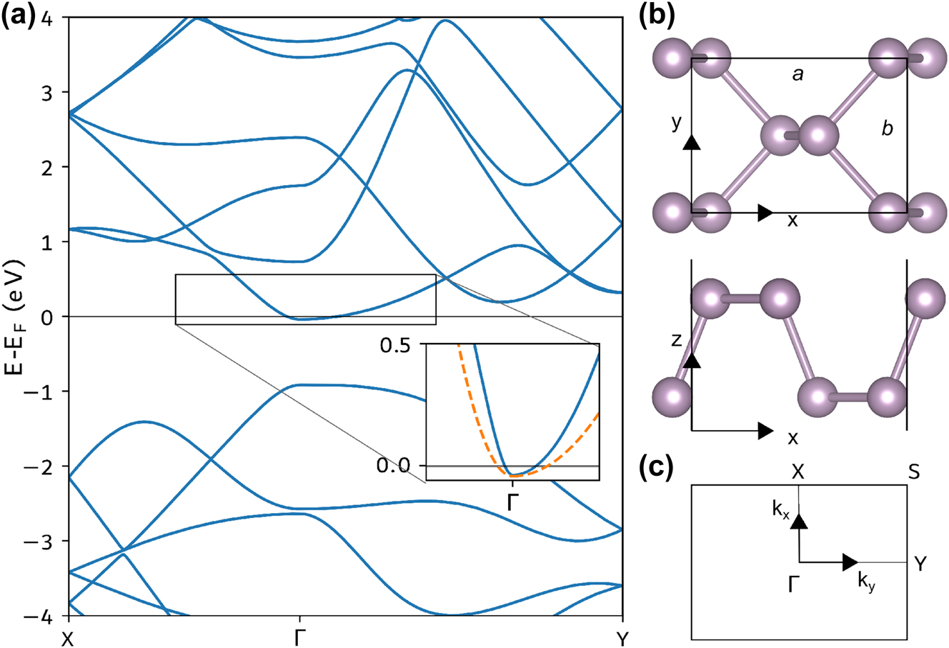
Electronic energy band structure of phosphorene. Panel (a) shows the band structure of extended monolayer phosphorene with doping charge carrier density n = 1 × 10¹³ cm⁻². The inset shows the conduction band along the Γ–X and Γ–Y directions of the first Brillouin zone (BZ) together with the parabolic bands (orange dashed lines) resulting from the fitted effective masses extracted from Figure 2. Panel (b) shows the unit cell of the 2D phosphorene crystal seen from above (top) and the side (bottom). Panel (c) shows the first BZ of the 2D crystal.

Figure 2:

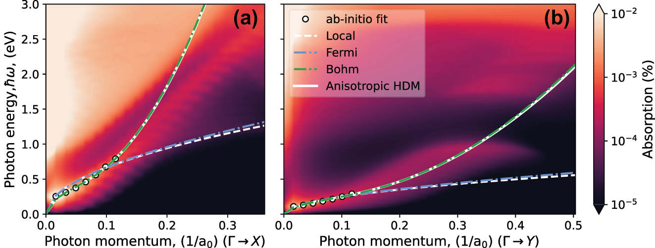
Density plot of the absorption obtained from ab initio calculations as a function of the photon energy ℏω and the photon wavenumber q with zero magnetic field. Panel (a) shows variations of q along the Γ–X direction in the Brillouin zone of the electronic-structure problem, while panel (b) is for the Γ–Y direction. In both panels, results for the dispersion relation from the hydrodynamic model (Eq. (18)) are superimposed, showing both the local approximation (dashed white line), the additional effect of Bohm’s potential (dash-dotted green line), the Fermi pressure (dash-dotted blue line), and the combined effects of Bohm’s potential and the Fermi pressure (solid white line). Maxima in absorption from the first principles calculation at low momenta are used for fitting of the effective masses (circles).

Ground-state DFT using the PBE functional is known to significantly underestimate the band gap of 2D materials, as the method excludes the many-body effects, which result in a significantly reduced screening. In these calculations, we obtain a band gap of 0.89 eV, which should be compared to experimental measurements yielding a gap size of 2 eV [64]. However, since many-body calculations using the GW method mainly result in a nearly constant energy correction of the conduction band [65], the effective masses and plasmon dispersion are not expected to differ much from what we extract within the single-particle approximation.

3.2 Comparison of the first principles and hydrodynamic approaches

Figure 2 presents the ab initio results for plasmons in phosphorene (colormap), as described in the previous section, considering n ₀ = 10¹³ cm⁻². Additionally, we show the analytical results derived from Eq. (18) for a zero magnetic field (B _z = 0), incorporating different nonlocal terms of f _q . The effective masses m _x and m _y were determined by fitting the plasmon dispersion at low momenta in both the zigzag and armchair directions, yielding m _x = 0.464m ₀, m _y = 2.394m ₀. The parabolic bands resulting from these effective masses are shown by the dashed orange lines on the inset of Figure 1a. It can be seen that the conduction band along the Γ–X direction is almost linear close to the Γ-point, resulting in a poorer fit to the parabolic band along this direction. Including the Bohm potential, a nonlocal contribution, enables an accurate description of the ab initio plasmon dispersion, whereas the Drude term, which follows a square root dependence on the wavenumber, fails to do so. Additionally, for the electronic density considered, the contribution from Fermi degeneracy pressure is negligible.

The local-response approximation holds for the Γ–Y direction for larger values of wavenumber than in the Γ–X direction. This occurs due to the effective mass dependence on Eq. (21); the lighter mass direction (Γ–X) results in a greater kinetic energy, implying an increased Bohm’s term and, therefore, more significant nonlocal effects.

3.3 Magnetoplasmons

We begin this section by examining the nonlocal effects on plasmon dispersion governed by Eq. (16), using the fitted effective masses from the previous section. In Figure 3a, we present a colormap of the relative difference in plasmon dispersion, Δω/ω _D , where ω _D represents the Drude dispersion, obtained by setting f _q = 0 in Eq. (16). The quantity Δω ≡ ω _p − ω _D is shown as a function of the electronic density n ₀ and the wavenumber q _y . We observe that nonlocal effects are present in the low electronic density and high wavenumber region, such as that for n ₀ < 10¹⁵ cm⁻² and q _y > 60 μm⁻¹, the nonlocal corrections are not negligible. A similar conclusion could be obtained for the q _x dependence, but nonlocal effects become important at smaller q _x when compared to q _y due to m _x < m _y .

Figure 3:

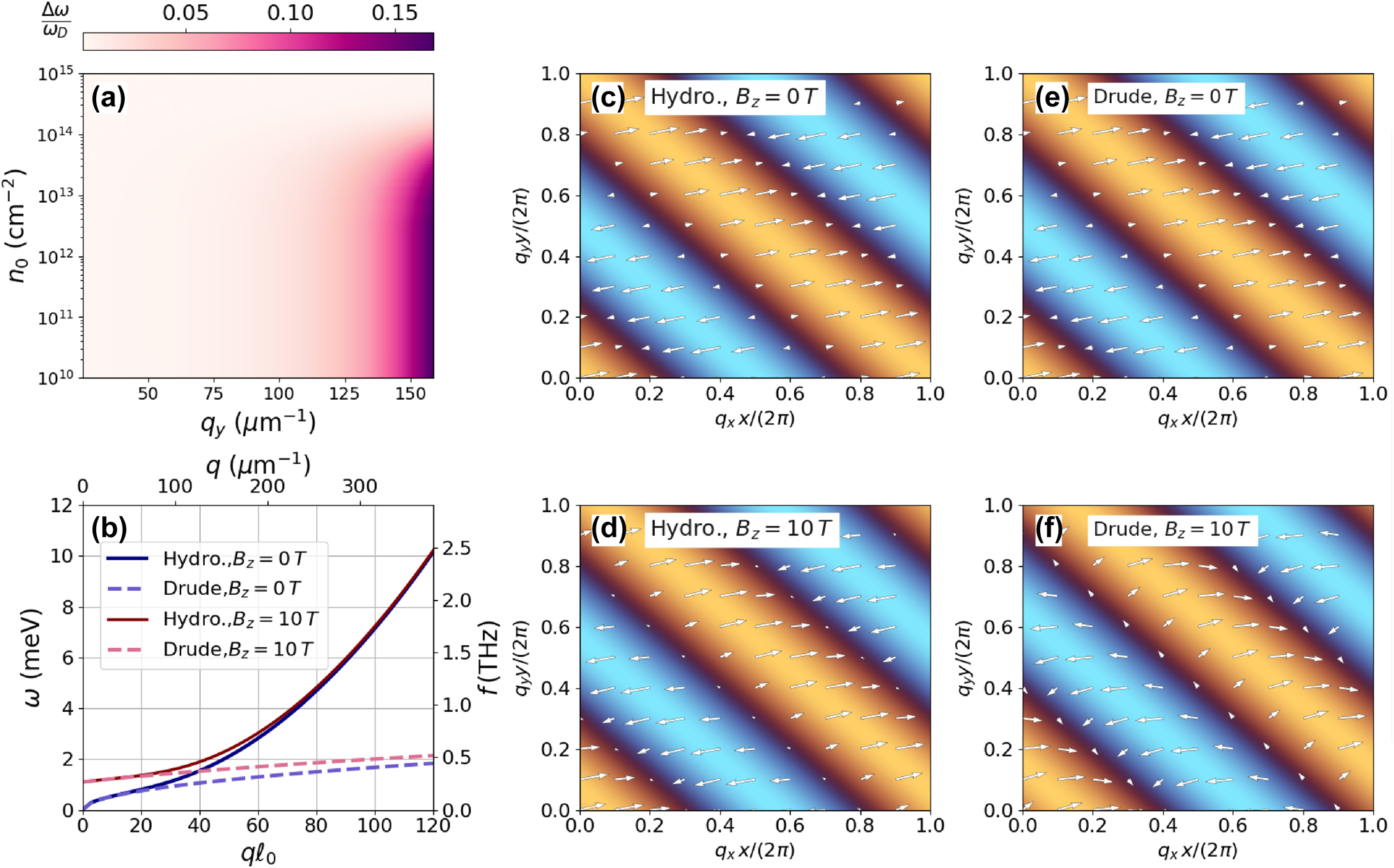
Panel (a) is a density plot of Δω/ω ₀ – the relative difference between the nonlocal and local plasmon dispersion of phosphorene – as function of the electronic density n ₀ and the plasmon wavenumber q _y in the zigzag direction. Panel (b) shows the magnetoplasmon dispersion relation for phosphorene – frequency f = ω/2π versus wavenumber q – comparing the nonlocal hydrodynamic model (solid lines) to the local Drude model (dashed lines) for both B _z = 0 T (blue coloring) and B _z = 10 T (red coloring). The effective mass was obtained from the ab initio fitting and n ₀ = 10⁹ cm⁻². We consider a direction that makes a 45° angle with either the zigzag or armchair direction. Panels (c–f) show Quiver plots of the plasmon velocity field and colormap of the charge-density fluctuation for phosphorene for qℓ ₀ = 90, as a function of the real-space coordinates x and y for different magnetic fields, for both the nonlocal hydrodynamic and the local Drude models. We use the effective mass obtained from the ab initio fitting and n ₀ = 10⁹ cm⁻².

The magnetoplasmon spectrum derived from Eq. (18) is displayed in Figure 3b. In the presence of a magnetic field, we observe that the deviation of the hydrodynamic (solid curves) and Drude model (dashed curves) shifts toward higher wavenumbers. This is a consequence of Bohm’s term, which corresponds to the kinetic energy inside the brackets in Eq. (18), and adds quartic terms inside the square root of the plasmon frequency; this explains the deviation between the hydrodynamic and Drude’s models for larger wavenumbers. The behavior is different for the plasmon velocity fields. In Figure 3c–f, we present a quiver plot of the normalized velocity fields obtained from the nontrivial solutions of Eq. (16). The colormap represents the normalized charge density calculated from the continuity equation (14) for both finite and zero magnetic fields, considering the nonlocal hydrodynamic and local Drude (f _q = 0) models.

In the case of a vanishing magnetic field, considered in Figure 3c and e, we can show that the nontrivial solution of Eq. (16) simplifies to q _y u _1,x /m _y − q _x u _1,y /m _x = 0 and does not depend on f _q , such that the velocity field (u _1,x , u _1,y ) is parallel to the vector (q _x /m _x , q _y /m _y ) in both cases: Drude and hydrodynamic models. In this case, the velocity field oscillates perpendicular to the charge density wavefront. However, for finite B _z , the velocity field acquires a dependence on nonlocal corrections, as can be seen by comparing Figure 3d and f. In the absence of nonlocal corrections, as shown in Figure 3f, the presence of the magnetic field causes the velocity field to become oblique to the charge density wavefront. In the nonlocal hydrodynamic model, as illustrated in Figure 3d, nonlocal effects decrease the transverse component of the velocity field, thus diminishing the magnetic field effect.

3.4 Effects of nonlocality: polaritonic spectrum

The coupling of light with plasmons gives rise to surface plasmon-polaritons (SPPs). In the case of BP, the anisotropic nature of the interband response indicates the existence of in-plane hyperbolic SPPs [66]. In this section, we examine a slab of BP with negligible thickness. The total optical conductivity of BP is expressed as the sum of a hydrodynamic component given by Eq. (28) and an additional contribution from interband transitions that is not accounted for in the hydrodynamic model,

Here, the interband conductivity σ i inter ( ω ) = i ϵ 0 ϵ i t is given in terms of constant relative permittivities ϵ _i and the BP slab thickness t, which we take from data extracted from IR absorption experiments [66]: ϵ _x = 12.5, ϵ _y = 10.2, and t = 2.9 nm. In Figure 4, we show the dielectric function

for both armchair and zigzag directions of BP, showing in the shaded region the BP Reststrahlen band, i.e., when Re{ϵ _xx } × Re{ϵ _yy } < 0. In this section, for the thin-layer BP, we will consider the effective masses of Ref. [66], μ _x = 0.14 (AC) and μ _y = 0.71 (ZZ).

Figure 4:

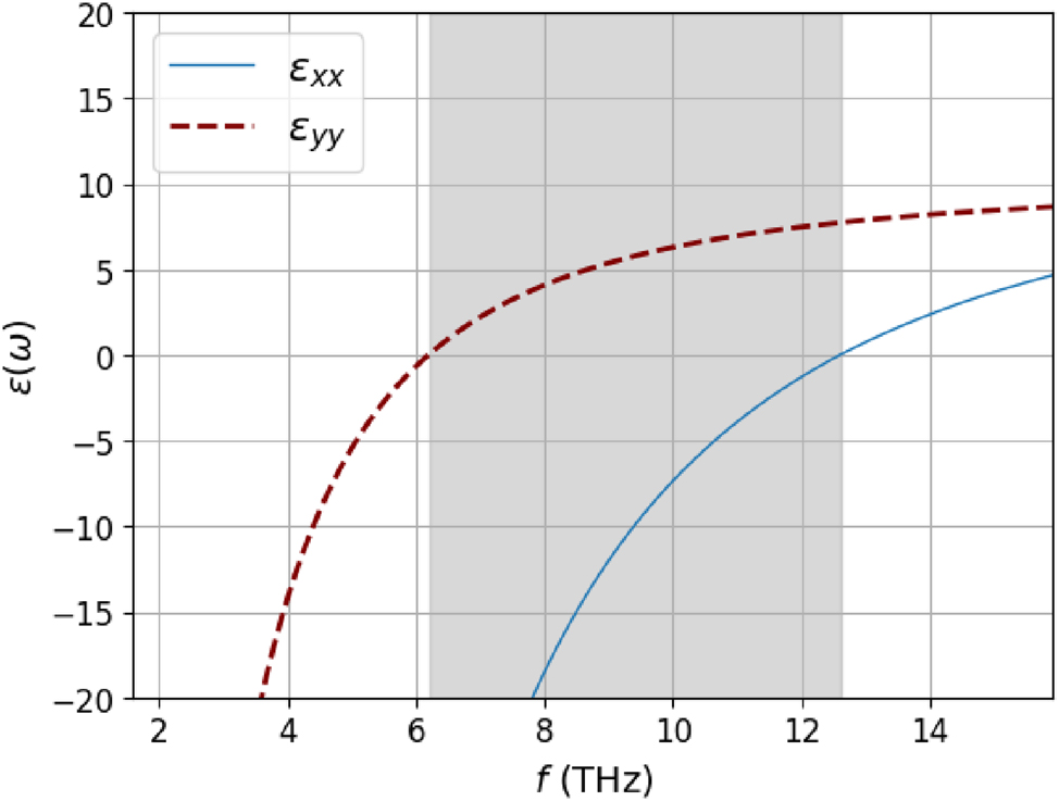
Black phosphorus anisotropic dielectric function ϵ(ω), calculated from Eq. (30) for an electronic density n ₀ = 10¹² cm⁻². The Reststrahlen band with Re{ϵ _xx } × Re{ϵ _yy } < 0 is highlighted in gray.

The presence of SPPs can be seen in the TM loss function, which is calculated from the imaginary part of the Fresnel coefficient r _p,p (see Appendix A for the derivation):

where

with μ 0 = c − 2 ϵ 0 − 1 being the vacuum permeability (not to be confused with relative effective masses μ _x and μ _y ), while σ ̃ i j are the components of the rotated conductivity tensor σ ̃ = R ϕ T σ R ϕ . Here, R _ϕ is the 2D rotation matrix along the z axis and tanϕ = q _x /q _y .

In Figure 5a and b, we show the TM loss function Im{r _p,p } for the surface plasmon-polariton isofrequency for f = 9.0 THz, which lies within the Reststrahlen band when n ₀ = 10¹² cm⁻². The results are shown for both the nonlocal hydrodynamic and local Drude models, including losses (see Appendix B), where we fixed the damping rate at ℏγ = 1.0 meV. The models exhibit markedly different qualitative behaviors. While the local Drude model predicts the existence of hyperbolic modes, these modes completely vanish when nonlocal effects are taken into account. Instead, the isofrequency transitions toward what is expected for a typical anisotropic surface plasmon-polariton. This behavior can be understood by analyzing Eq. (28); the increase in wavenumber alters the sign of the imaginary part of the eigenvalues of the conductivity tensor due to its dependence on q.

Figure 5:

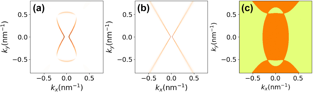
Panels (a) and (b) show density plots of the loss function Im{r _pp (q, ω)} as a function of q for a BP thin film at f = ω/2π = 9.0 THz calculated using Eq. (31). Panel (a) is for the nonlocal hydrodynamic model, while panel (b) is for the local Drude model. Panel (c) is a zero-contour plot of Im{λ ₁ λ ₂} in wavenumber space, separating positive regimes (in yellow) from negative regimes (in orange). The plot is for a photon frequency f = 9.0 THz, and the eigenvalues λ _1,2 are those of the optical conductivity tensor matrix (Eq. (29)).

In Figure 5c, we illustrate the sign of the imaginary part of the product of the eigenvalues of the conductivity tensor (29). When the sign is negative, we can expect the presence of hyperbolic modes. Conversely, when the sign is positive, we may observe elliptic modes (if both imaginary parts are negative) or no modes at all (if both are positive). By comparing Figure 5b and c, we observe that in the hyperbolic branches of the Drude model, the hydrodynamic model alters the sign of Im{λ ₁ λ ₂}, thereby inhibiting the formation of hyperbolic modes. Similar conclusions have been drawn for SPPs in BP using the Kubo formula for optical conductivity [27], considering an effective Hamiltonian [67]. It was observed that the inclusion of nonlocal effects significantly alters the isofrequencies, preventing the emergence of hyperbolic modes. A similar conclusion has been reached in the context of hyperbolic metamaterials [68] (and eventually also natural hyperbolic materials [69]), where the incorporation of nonlocal effects strongly renormalizes the spectrum in the high wavenumber limit.

3.5 Dipoles and Purcell effect

One possible way to launch surface plasmon-polaritons is through the use of an emitting dipole [70], where the near-field of the dipole couples with the light–matter modes. In the scanning near-field optical microscopy (SNOM), the atomic-force microscopy (AFM) tip can be modeled as a point dipole [71]; in this case, the tip supports evanescent modes that are excited by an incoming laser and can couple to SPP modes. To obtain the electromagnetic field in the presence of a dipole, we use the dyadic Green function formalism [72], in which, for the case of light impinging on an anisotropic medium, it was obtained elsewhere [73]:

where r _ss , r _sp , r _ps , and r _pp are the Fresnel coefficients calculated in Appendix A, and the matrix M _jk is defined in Appendix C. However, the numerical calculation of the integral above is challenging due to the presence of the SPP poles in the Fresnel coefficients. The electric field for an electric dipole that oscillates with frequency ω located at the position r′ is obtained from the dyadic Green’s function as:

where d is the electric dipole moment and G ₀ is the free-space dyadic Green’s function.

For simplicity, we henceforth consider an electric dipole oriented along the z-axis; accordingly, the reflected electric field in the z-direction is given by

The integral is dominated by the plasmon-pole, which can be obtained from the Fresnel coefficient denominator (32) as the solution of

For the case of plasmons, this pole is dominated by the TM part, i.e., the above equation has approximately the same roots as:

and we approximate the r _pp Fresnel coefficient as

with ω _SPP(q) being the solution of Eq. (37) and F(ω) corresponding to the residue of the plasmon-polariton pole,

We next shift the pole by an infinitesimal amount and take the imaginary part:

Now to simplify the integral in Eq. (35), we rewrite it in polar coordinates and make the change of variables k _‖ = k ₀ s. Considering s ≫ 1, we obtain for a dipole placed at (x′, y′, z′) = (0, 0, z ₀) that

To illustrate our point, we will for simplicity neglect the Bohm potential (7), so that we can obtain an analytical expression for the isofrequencies of the dispersion relation, as detailed in Appendix D. The relation between s and the polar angle ϕ, obtained after integrating over ϕ using the Dirac delta function, is

where we have defined

and C p = π n 0 λ ̃ c 2 μ x μ y , A = 4 π α λ ̃ c n 0 k 0 μ x μ y , ϵ m = ϵ x + ϵ y 2 , Δϵ = ϵ _y − ϵ _x , μ r − 1 = μ x − 1 + μ y − 1 , Δμ = μ _y − μ _x , with α the fine structure constant and λ ̃ c the reduced Compton wavelength. Based on this, the electric field in Eq. (41) can be expressed – after integrating in ϕ using Dirac’s delta function – as a single quadrature that can be easily computed numerically:

where the summation in ϕ _H corresponds to all nondegenerate solutions of Eq. (42) and the integral is limited to the intervals where |cos2ϕ _H (s)| ≤ 1. Using the symmetry of the solutions, we can write the above integral as:

with

For the case of the local response Drude model, Eq. (42) simplifies to:

In Figure 6a and b, we show the comparison between the hydrodynamic (including only the Fermi pressure term) and Drude models, for the frequency ω/(2π) = 9 THz, that lies inside the Reststrahlen band. While the Drude model predicts extremely canalized plasmons that propagate in the direction dictated by the hyperbolic dispersion, the hydrodynamic model shows closed wavefronts propagating in all directions.

Figure 6:

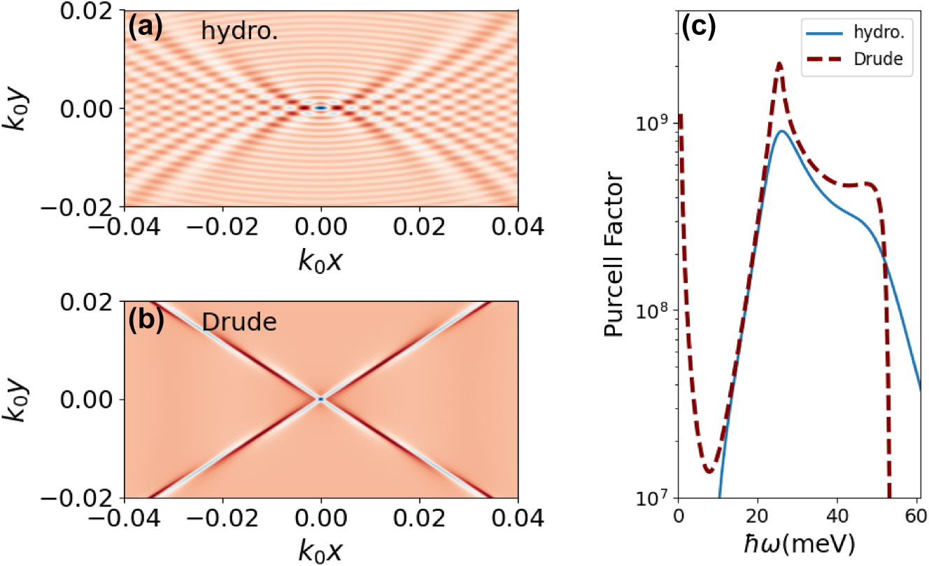
Panels (a) and (b) show plasmonics wakes induced by an electric dipole aligned with the z-axis with a frequency ω/(2π) = 9 THz. The colormap shows the electric field in the z-direction at the surface of the BP. Panel (a) is the hydrodynamic model, and panel (b) is the Drude model. Panel (c) compares the Purcell factor computed from the hydrodynamic model (solid line) and Drude model (dashed line) as a function of the frequency of the electric dipole. In all the plots, the dipole-BP sheet distance is z ₀ = 3.0 nm and the BP electronic density is n ₀ = 10¹² cm⁻².

The presence of a 2D material that supports plasmons changes a quantum emitter radiative decay through the Purcell effect [74]. The study of the Purcell effect in phosphorene, including strain, was done before [75] but neglecting nonlocal effects, i.e., the phosphorene optical conductivity was calculated using a tight-binding model without dependence on the in-plane wavenumber, or, when including nonlocal effects, the anisotropy was averaged [76]. The Purcell factor for a dipole aligned in the z-direction can be calculated using the following equation [75]:

The details of the numerical calculation of the Purcell factor are given in Appendix E, and the results are shown in Figure 6c. While the Drude model predicts a peak in the zero frequency, this peak disappears in the hydrodynamic model. The peaks of the Drude model also decrease by almost a factor of 3. For higher frequencies, the hydrodynamic model predicts a higher Purcell factor.

References

[1] M. F. Weber, C. A. Stover, L. R. Gilbert, T. J. Nevitt, and A. J. Ouderkirk, “Giant birefringent optics in multilayer polymer mirrors,” Science, vol. 287, no. 5462, pp. 2451–2456, 2000.10.1126/science.287.5462.2451Search in Google Scholar PubMed
[2] M. Born and E. Wolf, Principles of Optics: Electromagnetic Theory of Propagation, Interference and Diffraction of Light, London, Cambridge University Press, 2013.Search in Google Scholar
[3] T. E. Furtak and D. W. Lynch, “Anisotropic interband effects in electroreflectance of Ag,” Phys. Rev. Lett., vol. 35, no. 14, pp. 960–963, 1975.10.1103/PhysRevLett.35.960Search in Google Scholar
[4] A. Tadjeddine, D. Kolb, and R. Kötz, “The study of single crystal electrode surfaces by surface plasmon excitation,” Surf. Sci., vol. 101, no. 1, pp. 277–285, 1980.10.1016/0039-6028(80)90621-4Search in Google Scholar
[5] A. Friedrich, B. Pettinger, D. M. Kolb, G. Lüpke, R. Steinhoff, and G. Marowsky, “An in situ study of reconstructed gold electrode surfaces by second harmonic generation,” Chem. Phys. Lett., vol. 163, no. 2, pp. 123–128, 1989.10.1016/0009-2614(89)80022-3Search in Google Scholar
[6] G. Lüpke, G. Marowsky, R. Steinhoff, A. Friedrich, B. Pettinger, and D. M. Kolb, “Symmetry superposition studied by surface second-harmonic generation,” Phys. Rev. B, vol. 41, no. 10, pp. 6913–6919, 1990.10.1103/PhysRevB.41.6913Search in Google Scholar PubMed
[7] S. Boroviks, et al.., “Anisotropic second-harmonic generation from monocrystalline gold flakes,” Opt. Lett., vol. 46, no. 4, pp. 833–836, 2021.10.1364/OL.413003Search in Google Scholar PubMed
[8] P. Ajayan, P. Kim, and K. Banerjee, “Two dimensional van der Waals materials,” Phys. Today, vol. 69, no. 9, pp. 38–44, 2016.10.1063/PT.3.3297Search in Google Scholar
[9] P. Li, et al.., “Hyperbolic phonon-polaritons in boron nitride for near-field optical imaging and focusing,” Nat. Commun., vol. 6, no. 1, p. 7507, Jun 2015. https://doi.org/10.1038/ncomms8507.Search in Google Scholar PubMed PubMed Central
[10] S. Dai, et al.., “Phonon polaritons in monolayers of hexagonal boron nitride,” Adv. Mater., vol. 31, no. 37, p. 1806603, 2019.10.1002/adma.201806603Search in Google Scholar PubMed
[11] Z. Zheng, et al.., “Highly confined and tunable hyperbolic phonon polaritons in van der Waals semiconducting transition metal oxides,” Adv. Mater., vol. 30, no. 13, p. 1705318, 2018.10.1002/adma.201705318Search in Google Scholar PubMed
[12] J. Taboada-Gutiérrez, et al.., “Unveiling the mechanism of phonon-polariton damping in α-MoO3,” ACS Photonics, vol. 11, no. 9, pp. 3570–3577, 2024.10.1021/acsphotonics.4c00485Search in Google Scholar PubMed PubMed Central
[13] N. C. Passler, et al.., “Hyperbolic shear polaritons in low-symmetry crystals,” Nature, vol. 602, no. 7898, pp. 595–600, Feb 2022. https://doi.org/10.1038/s41586-021-04328-y.Search in Google Scholar PubMed PubMed Central
[14] A. Kumar, T. Low, K. H. Fung, P. Avouris, and N. X. Fang, “Tunable light–matter interaction and the role of hyperbolicity in graphene–hbn system,” Nano Lett., vol. 15, no. 5, pp. 3172–3180, 2015.10.1021/acs.nanolett.5b01191Search in Google Scholar PubMed
[15] I. D. Barcelos, et al.., “Ultrabroadband nanocavity of hyperbolic phonon–polaritons in 1D-like α-MoO3,” ACS Photonics, vol. 8, no. 10, pp. 3017–3026, Oct 2021. https://doi.org/10.1021/acsphotonics.1c00955.Search in Google Scholar
[16] Z. Liu and K. Aydin, “Localized surface plasmons in nanostructured monolayer black phosphorus,” Nano Lett., vol. 16, no. 6, pp. 3457–3462, 2016.10.1021/acs.nanolett.5b05166Search in Google Scholar PubMed
[17] G. Venturi, A. Mancini, N. Melchioni, S. Chiodini, and A. Ambrosio, “Visible-frequency hyperbolic plasmon polaritons in a natural van der Waals crystal,” Nat. Commun., vol. 15, no. 1, p. 9727, Nov 2024. https://doi.org/10.1038/s41467-024-53988-7.Search in Google Scholar PubMed PubMed Central
[18] F. L. Ruta, et al.., “Good plasmons in a bad metal,” Science, vol. 387, no. 6735, pp. 786–791, 2025.10.1126/science.adr5926Search in Google Scholar PubMed
[19] A. A. Maradudin, J. R. Sambles, and W. L. Barnes, Modern Plasmonics, vol. 4, Amsterdam, Elsevier, 2014.Search in Google Scholar
[20] H. Wang, et al.., “Planar hyperbolic polaritons in 2D van der Waals materials,” Nat. Commun., vol. 15, no. 1, p. 69, Jan 2024. https://doi.org/10.1038/s41467-023-43992-8.Search in Google Scholar PubMed PubMed Central
[21] P. A. D. Gonçalves, N. Stenger, J. D. Cox, N. A. Mortensen, and S. Xiao, “Strong light–matter interactions enabled by polaritons in atomically thin materials,” Adv. Opt. Mater., vol. 8, no. 5, p. 1901473, 2020.10.1002/adom.201901473Search in Google Scholar
[22] N. A. Mortensen, “Mesoscopic electrodynamics at metal surfaces,” Nanophotonics, vol. 10, no. 10, pp. 2563–2616, 2021.10.1515/nanoph-2021-0156Search in Google Scholar
[23] F. Monticone, et al.., “Roadmap on nonlocality in photonic materials and metamaterials,” Opt. Mater. Express, vol. 15, no. 7, pp. 1544–1708, 2025.10.1364/OME.550403Search in Google Scholar
[24] S. Boroviks, et al.., “Extremely confined gap plasmon modes: When nonlocality matters,” Nat. Commun., vol. 13, no. 1, p. 3105, 2022. https://doi.org/10.1038/s41467-022-30737-2.Search in Google Scholar PubMed PubMed Central
[25] M. B. Lundeberg, et al.., “Tuning quantum nonlocal effects in graphene plasmonics,” Science, vol. 357, no. 6347, pp. 187–191, 2017.10.1126/science.aan2735Search in Google Scholar PubMed
[26] E. J. C. Dias, et al.., “Probing nonlocal effects in metals with graphene plasmons,” Phys. Rev. B, vol. 97, no. 24, p. 245405, 2018.10.1103/PhysRevB.97.245405Search in Google Scholar
[27] D. Correas-Serrano, J. S. Gomez-Diaz, A. A. Melcon, and A. Alù, “Black phosphorus plasmonics: anisotropic elliptical propagation and nonlocality-induced canalization,” J. Opt., vol. 18, no. 10, p. 104006, 2016. https://doi.org/10.1088/2040-8978/18/10/104006.Search in Google Scholar
[28] C. A. Ullrich, Time-Dependent Density-Functional Theory: Concepts and Applications, Oxford, New York, Oxford University Press, 2011.10.1093/acprof:oso/9780199563029.001.0001Search in Google Scholar
[29] C. Ciracì, “Current-dependent potential for nonlocal absorption in quantum hydrodynamic theory,” Phys. Rev. B, vol. 95, no. 24, p. 245434, 2017.10.1103/PhysRevB.95.245434Search in Google Scholar
[30] G. Barton, “Some surface effects in the hydrodynamic model of metals,” Rep. Prog. Phys., vol. 42, no. 6, p. 963, 1979. https://doi.org/10.1088/0034-4885/42/6/001.Search in Google Scholar
[31] Q. Zhou, W. Li, Z. He, P. Zhang, and X.-W. Chen, “Quantum hydrodynamic model for noble metal nanoplasmonics,” Phys. Rev. B, vol. 107, no. 20, p. 205413, 2023. https://doi.org/10.1103/PhysRevB.107.205413.Search in Google Scholar
[32] T. V. Teperik, P. Nordlander, J. Aizpurua, and A. G. Borisov, “Robust subnanometric plasmon ruler by rescaling of the nonlocal optical response,” Phys. Rev. Lett., vol. 110, p. 263901, 2013.10.1103/PhysRevLett.110.263901Search in Google Scholar PubMed
[33] F. De Luca, M. Ortolani, and C. Ciracì, “Free electron nonlinearities in heavily doped semiconductors plasmonics,” Phys. Rev. B, vol. 103, no. 11, p. 115305, 2021. https://doi.org/10.1103/PhysRevB.103.115305.Search in Google Scholar
[34] A. J. Chaves, N. M. R. Peres, G. Smirnov, and N. A. Mortensen, “Hydrodynamic model approach to the formation of plasmonic wakes in graphene,” Phys. Rev. B, vol. 96, no. 19, p. 195438, 2017. https://doi.org/10.1103/PhysRevB.96.195438.Search in Google Scholar
[35] T. C. Barbosa, A. J. Chaves, R. O. Freitas, L. C. Campos, and I. D. Barcelos, “Ultra-confined plasmons reveal moiré patterns in a twisted bilayer graphene–talc heterostructure,” Nanoscale, vol. 17, no. 15, pp. 9205–9212, 2025.10.1039/D4NR04532GSearch in Google Scholar
[36] C. Ciracì, et al.., “Probing the ultimate limits of plasmonic enhancement,” Science, vol. 337, no. 6098, pp. 1072–1074, 2012.10.1126/science.1224823Search in Google Scholar PubMed PubMed Central
[37] P. Zhang, C. Tserkezis, and N. A. Mortensen, “Quantum-hydrodynamic modal perspective on plasmonic gap structures,” J. Phys. Chem. C, vol. 129, no. 7, pp. 3667–3675, 2025. https://doi.org/10.1021/acs.jpcc.4c08232.Search in Google Scholar
[38] J. Baxter, A. C. Lesina, and L. Ramunno, “Parallel FDTD modeling of nonlocality in plasmonics,” IEEE Trans. Antenn. Propag., vol. 69, no. 7, pp. 3982–3994, 2021.10.1109/TAP.2020.3044579Search in Google Scholar
[39] H. Du and C. Liu, “An improved FDTD method to calculate nonlocal response in plasmonics,” IEEE Trans. Antenn. Propag., vol. 72, no. 3, pp. 2592–2599, 2024.10.1109/TAP.2024.3363445Search in Google Scholar
[40] K. R. Hiremath, L. Zschiedrich, and F. Schmidt, “Numerical solution of nonlocal hydrodynamic Drude model for arbitrary shaped nanoplasmonic structures using nédélec finite elements,” J. Comput. Phys., vol. 231, no. 17, pp. 5890–5896, 2012.10.1016/j.jcp.2012.05.013Search in Google Scholar
[41] M. Moeferdt, T. Kiel, T. Sproll, F. Intravaia, and K. Busch, “Plasmonic modes in nanowire dimers: A study based on the hydrodynamic Drude model including nonlocal and nonlinear effects,” Phys. Rev. B, vol. 97, no. 7, p. 075431, 2018.10.1103/PhysRevB.97.075431Search in Google Scholar
[42] L. Li, S. Lanteri, N. A. Mortensen, and M. Wubs, “A hybridizable discontinuous Galerkin method for solving nonlocal optical response models,” Comput. Phys. Commun., vol. 219, pp. 99–107, 2017.10.1016/j.cpc.2017.05.012Search in Google Scholar
[43] P. Cosme and H. Terças, “Terahertz laser combs in graphene field-effect transistors,” ACS Photonics, vol. 7, no. 6, pp. 1375–1381, 2020.10.1021/acsphotonics.0c00313Search in Google Scholar
[44] X. Hua, D. Sun, D. Liu, and N. Ma, “The double-layer graphene surface plasmon-polaritons spectrum in hydrodynamic model,” Plasmonics, vol. 20, no. 3, pp. 1183–1191, 2025. https://doi.org/10.1007/s11468-024-02368-4.Search in Google Scholar
[45] A. Moradi and N. Türker Tokan, “Screened plasmons of graphene near a perfect electric conductor,” J. Appl. Phys., vol. 134, no. 15, p. 153103, 2023.10.1063/5.0172268Search in Google Scholar
[46] S. Ahn and S. Das Sarma, “Theory of anisotropic plasmons,” Phys. Rev. B, vol. 103, no. 4, p. L041303, 2021. https://doi.org/10.1103/PhysRevB.103.L041303.Search in Google Scholar
[47] S. S. Cardoso, A. J. Chaves, N. A. Mortensen, and N. M. R. Peres, “Application of Madelung hydrodynamics to plasmonics and nonlinear optics in two-dimensional materials,” Phys. Rev. A, vol. 111, no. 4, p. 043508, 2025.10.1103/PhysRevA.111.043508Search in Google Scholar
[48] M. Scalora, et al.., “Second- and third-harmonic generation in metal-based structures,” Phys. Rev. A, vol. 82, no. 4, p. 043828, 2010. https://doi.org/10.1103/PhysRevA.82.043828.Search in Google Scholar
[49] I. Gasser and P. A. Markowich, “Quantum hydrodynamics, Wigner transforms, the classical limit,” Asymptot. Anal., vol. 14, no. 2, pp. 97–116, 1997.10.3233/ASY-1997-14201Search in Google Scholar
[50] E. Madelung, “Quantum theory in hydrodynamical form,” Z. Phys., vol. 40, p. 322, 1927.10.1007/BF01400372Search in Google Scholar
[51] A. L. Fetter, “Edge magnetoplasmons in a bounded two-dimensional electron fluid,” Phys. Rev. B, vol. 32, no. 12, pp. 7676–7684, 1985.10.1103/PhysRevB.32.7676Search in Google Scholar
[52] A. L. Fetter, “Magnetoplasmons in a two-dimensional electron fluid: Disk geometry,” Phys. Rev. B, vol. 33, no. 8, pp. 5221–5227, 1986.10.1103/PhysRevB.33.5221Search in Google Scholar PubMed
[53] F. Xia, H. Wang, J. C. M. Hwang, A. H. Castro Neto, and L. Yang, “Black phosphorus and its isoelectronic materials,” Nat. Rev. Phys., vol. 1, no. 5, pp. 306–317, 2019.10.1038/s42254-019-0043-5Search in Google Scholar
[54] V. Tran, R. Soklaski, Y. Liang, and L. Yang, “Layer-controlled band gap and anisotropic excitons in few-layer black phosphorus,” Phys. Rev. B, vol. 89, no. 23, p. 235319, 2014. https://doi.org/10.1103/PhysRevB.89.235319.Search in Google Scholar
[55] X. Wang and S. Lan, “Optical properties of black phosphorus,” Adv. Opt. Photonics, vol. 8, no. 4, pp. 618–655, 2016.10.1364/AOP.8.000618Search in Google Scholar
[56] H. Liu, et al.., “Phosphorene: An unexplored 2D semiconductor with a high hole mobility,” ACS Nano, vol. 8, no. 4, pp. 4033–4041, 2014.10.1021/nn501226zSearch in Google Scholar PubMed
[57] J. P. Perdew, K. Burke, and M. Ernzerhof, “Generalized gradient approximation made simple,” Phys. Rev. Lett., vol. 77, no. 18, pp. 3865–3868, 1996.10.1103/PhysRevLett.77.3865Search in Google Scholar PubMed
[58] P. Giannozzi, et al.., “QUANTUM ESPRESSO: A modular and open-source software project for quantum simulations of materials,” J. Phys.: Condens. Matter, vol. 21, no. 39, p. 395502, 2009.10.1088/0953-8984/21/39/395502Search in Google Scholar PubMed
[59] D. R. Hamann, “Optimized norm-conserving Vanderbilt pseudopotentials,” Phys. Rev. B, vol. 88, no. 8, p. 085117, 2013.10.1103/PhysRevB.88.085117Search in Google Scholar
[60] M. J. van Setten, et al.., “The pseudodojo: Training and grading a 85 element optimized norm-conserving pseudopotential table,” Comput. Phys. Commun., vol. 226, pp. 39–54, 2018.10.1016/j.cpc.2018.01.012Search in Google Scholar
[61] A. Marini, C. Hogan, M. Grüning, and D. Varsano, “Yambo: An ab initio tool for excited state calculations,” Comput. Phys. Commun., vol. 180, no. 8, pp. 1392–1403, 2009.10.1016/j.cpc.2009.02.003Search in Google Scholar
[62] D. Sangalli, et al.., “Manybody perturbation theory calculations using the yambo code,” J. Phys.: Condens. Matter, vol. 31, no. 32, p. 325902, 2019.10.1088/1361-648X/ab15d0Search in Google Scholar PubMed
[63] T. Sohier, M. Calandra, and F. Mauri, “Density functional perturbation theory for gated two-dimensional heterostructures: Theoretical developments and application to flexural phonons in graphene,” Phys. Rev. B, vol. 96, no. 7, p. 075448, 2017.10.1103/PhysRevB.96.075448Search in Google Scholar
[64] L. Liang, J. Wang, W. Lin, B. G. Sumpter, V. Meunier, and M. Pan, “Electronic bandgap and edge reconstruction in phosphorene materials,” Nano Lett., vol. 14, no. 11, pp. 6400–6406, 2014.10.1021/nl502892tSearch in Google Scholar PubMed
[65] F. Ferreira and R. M. Ribeiro, “Improvements in the GW and Bethe-Salpeter equation calculations on phosphorene,” Phys. Rev. B, vol. 96, no. 11, p. 115431, 2017.10.1103/PhysRevB.96.115431Search in Google Scholar
[66] S. Biswas, et al.., “Tunable intraband optical conductivity and polarization-dependent epsilon-near-zero behavior in black phosphorus,” Sci. Adv., vol. 7, no. 2, p. eabd4623, 2021.10.1126/sciadv.abd4623Search in Google Scholar PubMed PubMed Central
[67] A. S. Rodin, A. Carvalho, and A. H. Castro Neto, “Strain-induced gap modification in black phosphorus,” Phys. Rev. Lett., vol. 112, no. 17, p. 176801, 2014. https://doi.org/10.1103/PhysRevLett.112.176801.Search in Google Scholar PubMed
[68] W. Yan, M. Wubs, and N. A. Mortensen, “Hyperbolic metamaterials: Nonlocal response regularizes broadband supersingularity,” Phys. Rev. B, vol. 86, no. 20, p. 205429, 2012. https://doi.org/10.1103/PhysRevB.86.205429.Search in Google Scholar
[69] M. N. Gjerding, R. Petersen, T. G. Pedersen, N. A. Mortensen, and K. S. Thygesen, “Layered van der Waals crystals with hyperbolic light dispersion,” Nat. Commun., vol. 8, no. 1, p. 320, 2017.10.1038/s41467-017-00412-ySearch in Google Scholar PubMed PubMed Central
[70] P. A. D. Gonçalves and N. M. Peres, An Introduction to Graphene Plasmonics, Singapore, World Scientific, 2016.10.1142/9948Search in Google Scholar
[71] F. Keilmann and R. Hillenbrand, “Near-field microscopy by elastic light scattering from a tip,” Philos. Trans. R. Soc. A, vol. 362, no. 1817, pp. 787–805, 2004.10.1098/rsta.2003.1347Search in Google Scholar PubMed
[72] L. Novotny and B. Hecht, Principles of Nano-Optics, Cambridge, Cambridge University Press, 2012.10.1017/CBO9780511794193Search in Google Scholar
[73] J. S. Gomez-Diaz, M. Tymchenko, and A. Alù, “Hyperbolic metasurfaces: Surface plasmons, light-matter interactions, and physical implementation using graphene strips,” Opt. Mater. Express, vol. 5, no. 10, pp. 2313–2329, 2015.10.1364/OME.5.002313Search in Google Scholar
[74] B. A. Ferreira, B. Amorim, A. J. Chaves, and N. M. R. Peres, “Quantization of graphene plasmons,” Phys. Rev. A, vol. 101, no. 3, p. 033817, 2020.10.1103/PhysRevA.101.033817Search in Google Scholar
[75] P. P. Abrantes, W. J. M. Kort-Kamp, F. S. S. Rosa, C. Farina, F. A. Pinheiro, and T. P. Cysne, “Controlling electric and magnetic Purcell effects in phosphorene via strain engineering,” Phys. Rev. B, vol. 108, no. 15, p. 155427, 2023.10.1103/PhysRevB.108.155427Search in Google Scholar
[76] R. Petersen, T. G. Pedersen, and F. J. García de Abajo, “Nonlocal plasmonic response of doped and optically pumped graphene, MoS2, and black phosphorus,” Phys. Rev. B, vol. 96, no. 20, p. 205430, 2017. https://doi.org/10.1103/PhysRevB.96.205430.Search in Google Scholar
© 2025 the author(s), published by De Gruyter, Berlin/Boston
This work is licensed under the Creative Commons Attribution 4.0 International License.
Articles in the same Issue
- Frontmatter
- Editorial
- Editorial on special issue “The 11th International Conference on Surface Plasmon Photonics (SPP11)”
- Review
- Beyond limits: a tribute to Dai-Sik Kim’s academic legacy and vision
- Letters
- Meso-chiral optical properties of plasmonic nanoparticles: uncovering hidden chirality
- Modulation of the type and excitation region of plasmonic topological quasiparticles in a metasurface by tailoring the excitation light
- Research Articles