A point on discrete versus continuous state-space Markov chains

Mathias Muia; Martial Longla

doi:10.1515/demo-2025-0015

Article Open Access

A point on discrete versus continuous state-space Markov chains

Mathias Muia and Martial Longla

Published/Copyright: August 13, 2025

Published by

Become an author with De Gruyter Brill

Submit Manuscript Author Information Explore this Subject

From the journal Dependence Modeling Volume 13 Issue 1

Abstract

This article investigates the effects of discrete marginal distributions on copula-based Markov chains. We establish results on mixing properties and parameter estimation for a copula-based Markov chain model with Bernoulli( p ) marginal distributions, emphasizing some distinctions between continuous and discrete state-space Markov chains. We derive parameter estimators using the maximum-likelihood estimation (MLE) method and explore alternative estimators of p that are asymptotically equivalent to the MLE. Furthermore, we provide the asymptotic distributions of these parameter estimators. A simulation study is conducted to evaluate the performance of the various estimators for p . Additionally, we employ the likelihood ratio test to assess independence within the sequence.

Keywords: asymptotic normality; dependent Bernoulli trials; Frechet family of copulas; mixing for Markov chains

MSC 2010: 60J25

1 Introduction

Markov chain models have been widely used in the literature to represent the relationship between consecutive observations in a sequence of Bernoulli trials. Johnson and Klotz [18] employed a Markov chain generalization of a binomial model to analyze the crystal structure of a two-metal alloy in their metallurgical studies. Crow [9] investigated the applications of two-state Markov chains in telecommunications in his study focusing on approximating confidence intervals. Brainerd and Chang [7] used two-state Markov chains to address problems in linguistic analysis. These examples illustrate that Markov chain models can provide a solid foundation for modeling a wide range of two-state sequential phenomena.

Moreover, in the study of sequences consisting of different alternatives, there has been notable interest in using group or run tests to evaluate the randomness of the sequences. These tests are based on the count of changes between outcomes in the sequence, aiming to assess whether the sequence displays randomness (denoted as the null hypothesis, H 0 ) or exhibits a type of dependence similar to simple Markov chains (alternative hypothesis, H 1 ). These counts, denoted by n i j (where i , j = 0 , … , s denotes the states taken by the sequence), are commonly referred to as transition numbers of the sequence. The transition numbers have been widely used in the literature to construct run tests and in the estimation of model parameters (see David [10], Goodman [13], Anderson and Goodman [1], and Billingsley [4] for details). As used in this work, transition numbers prove to be very useful in computing the maximum-likelihood estimators (MLE) of parameters.

1.1 Copulas and Markov chains

A 2-copula is a bivariate function C : [ 0 , 1 ] 2 → [ 0 , 1 ] such that C ( 0 , u ) = C ( u , 0 ) = 0 , C ( u , 1 ) = C ( 1 , u ) = u , ∀ u ∈ [ 0 , 1 ] , and C ( u 1 , v 1 ) + C ( u 2 , v 2 ) − C ( u 1 , v 2 ) − C ( u 2 , v 1 ) ≥ 0 , ∀ [ u 1 , u 2 ] × [ v 1 , v 2 ] ⊂ [ 0 , 1 ] 2 . For some k ≥ 2 , let C 1 , … , C k be a set of k copulas and a 1 , … , a k a set of real constants such that a 1 + ⋯ + a k = 1 and 0 ≤ a i ≤ 1 for each i = 1 , … , k ; then, the sum given by C ( u , v ) = a 1 C 1 ( u , v ) + ⋯ + a k C k ( u , v ) is a copula referred to as the convex combination of C 1 , … , C k [24].

The copula C ( F ( x ) , G ( y ) ) = H ( x , y ) , of the random variables X and Y , is known to be unique if F and G are continuous; otherwise, C is uniquely determined on Range ( F ) × Range ( G ) [27]. In the recent past, copulas have gained popularity in the modeling of temporal dependence within Markov processes. This is because, when used to represent joint distributions of random variables, they enable the detection of possible correlations or links between variables [11]. A copula-based Markov chain is a stationary Markov chain generated by the copula of its consecutive states and an invariant distribution. Copula-based Markov chains enable the exploration of dependence and mixing properties inherent in Markov processes. This makes them an invaluable tool for investigations and allows for the study of scale-free measures of dependence while remaining invariant under monotonic transformations of the variables. Consequently, copula methods have drawn a lot of interest across diverse fields, including technology, finance, and the natural world.

This article focuses on a stationary Markov chain based on a copula from the Frechet family of copulas. The Fréchet family of copulas has the form

(1.1) C ( u , v ) = a M ( u , v ) + ( 1 − a − b ) Π ( u , v ) + b W ( u , v ) , a , b ≥ 0 , 0 ≤ a + b ≤ 1 ,

where Π ( u , v ) = u v is the independence copula and M ( u , v ) = min ( u , v ) and W ( u , v ) = max ( u + v − 1 , 0 ) are the Fréchet-Hoeffding upper and lower bounds, respectively. We study two cases: a continuous state-space Markov chain with uniform marginal distributions and a discrete state-space Markov chain with Bernoulli( p ) marginal distributions. MLEs of model parameters are derived in both cases, and their asymptotic distributions are provided. The likelihood ratio test is used to test for randomness in the model.

Studies involving inferential statistics for discrete cases closely similar to the one considered here have been presented in the works of Billingsley [4], Billingsley [3], Goodman [13], Klotz [19], Klotz [20], Price [29], Lindqvist [21], and others. Goodman [13] considered a single sequence of alternatives consisting of a long chain of observations to derive some long-sequence group tests. Klotz [20] presented small and large sample distribution theory for the sufficient statistics of a model for Bernoulli trials with Markov dependence. He provided estimators for the model parameters and showed that the uniform most powerful unbiased test of independence is the run test. On the other hand, Price [29] and Lindqvist [21] focused on estimating the model parameters only. Price [29] used Monte Carlo techniques to investigate finite sample properties for the parameters of a dependent Bernoulli process. Lindqvist [21] considered the weaker assumption of non-Markovian dependence and showed that the MLE, ( p ˆ , a ˆ ) is a strongly consistent and asymptotically normally distributed estimator for ( p , a ) . In the context of Klotz [20] and Lindqvist [21], as well as in this article, p represents the Bernoulli (frequency) parameter of a sequence of Bernoulli trials, while a is an additional dependence parameter. Lindqvist [21] further showed that ( p ˆ , a ˆ ) is asymptotically equivalent to ( p ¯ , a ¯ ) , where p ¯ is the sample mean and a ¯ is the empirical correlation coefficient of X t − 1 and X t .

The rest of this article is organized as follows: in Section 2, we introduce our model and detail the transition probabilities of the discrete Markov chain model considered. Mixing properties of the Markov chain model are discussed in Section 2.1. Section 3 covers parameter estimation, where we derive MLEs and their asymptotic distributions. In Section 4, we provide a test for independence in the sequence. This article concludes with a simulation study in Section 5.

2 Model

Consider a stationary Markov chain model based on the copula

(2.1) C ( u , v ) = a M ( u , v ) + ( 1 − a ) W ( u , v ) , a ∈ ( 0 , 1 ) .

Copula (2.1) is from the Frechet/Mardia family of copulas given by (1.1) with a + b = 1 . Note that a Mardia copula with a parameter θ ∈ [ − 1 , 1 ] is a Frechet copula with a + b = θ 2 . For details on these copula families, see Nelsen [27], Joe [17], or Durante and Sempi [12].

Longla [23] showed that a stationary Markov chain with copula (2.1) and uniform marginals has n -steps joint cumulative distribution function (cdf) of the form

(2.2) C n ( u , v ) = 1 ⁄ 2 [ 1 + ( 2 a − 1 ) n ] M ( u , v ) + 1 ⁄ 2 [ 1 − ( 2 a − 1 ) n ] W ( u , v ) .

If the marginals are Bernoulli( p ), the joint distributions can be characterized by the transition probabilities of the Markov chain and the stationary distribution. Note that Sklar’s theorem states that C is only identifiable on Ran ( F ) × Ran ( G ) . Theorem 1 provides the transition matrices for the Markov chain.

Theorem 1

Let X = ( X t ) t = 0 , … , n be a stationary Markov chain generated by copula (2.1) and Bernoulli( p ) marginals. Then, X has transition matrices given by

(2.3) A = a p + 1 − 2 p 1 − p p ( 1 − a ) 1 − p 1 − a a , p < 1 ⁄ 2 ,

and

(2.4) A = a 1 − a ( 1 − p ) ( 1 − a ) p a ( 1 − p ) + 2 p − 1 p , p ≥ 1 ⁄ 2 .

Proof

Due to stationarity of the Markov chain, P ( X t = 1 ) = 1 − P ( X t = 0 ) = p . It suffices to determine P ( X 0 = 0 , X 1 = 0 ) .

P ( X 0 = 0 , X 1 = 0 ) = P ( X 0 ≤ 0 , X 1 ≤ 0 ) = C ( 1 − p , 1 − p ) = a ( 1 − p ) + ( 1 − a ) max ( 1 − 2 p , 0 ) = a p + 1 − 2 p , if p < 1 ⁄ 2 a ( 1 − p ) , if p ≥ 1 ⁄ 2 ,

where the second equality follows from Sklar’s theorem (Sklar [30]). The rest of the probabilities are computed using the hypothesis that the Markov chain is stationary with Bern( p ) marginals. For p < 1 ⁄ 2 , the joint distribution is given in Table 1.

Using the definition of conditional probability, P ( X 1 = j ∣ X 0 = i ) = P ( X 1 = j , X 0 = i ) ⁄ P ( X 0 = i ) , in Table 1 we obtain transition matrix (2.3). A similar argument is used for p ≥ 1 ⁄ 2 to obtain transition matrix (2.4).□

Table 1

Distribution of ( X 0 , X 1 ) when p < 1 ⁄ 2

	X 1
X 0	0	1	P X 0 ( x )
0	a p + 1 − 2 p	p ( 1 − a )	1 − p
1	p ( 1 − a )	a p	p
P X 1 ( y )	1 − p	p	1

The statistical behavior of the distribution at p = 1 ⁄ 2 reflects a symmetric transition structure where the probability of transitioning between states is balanced by the parameter a . This symmetry simplifies the interpretation and analysis of the Markov chain, making it an interesting case for studying the dynamics governed by the mixture copula model.

Transition matrix (2.3) is similar to the one considered by Klotz [20]. In our case, we have a frequency parameter p = P ( X t = 1 ) and an additional dependence parameter a = P ( X t = 1 ∣ X t − 1 = 1 ) , when p < 1 ⁄ 2 or a = P ( X t = 0 ∣ X t − 1 = 0 ) , when p ≥ 1 ⁄ 2 . In Klotz [20], the condition max ( 0 , ( 2 p − 1 ) ⁄ p ) ≤ a ≤ 1 was required so that the transition probabilities of the model remain bounded between 0 and 1. The model presented in this work does not require this condition because the copula conditions sufficiently define the transition probabilities based on whether p < 1 ⁄ 2 or p ≥ 1 ⁄ 2 . Specifically, the transition probabilities remain bounded between 0 and 1 for any value of 0 < a < 1 , and they satisfy ∑ j p i j = 1 for j = 0 , 1 .

Proposition 2

The nth transition matrices for (2.3) and (2.4) are, respectively,

(2.5) A n = 1 − p + p a − p 1 − p n p − p a − p 1 − p n 1 − p − ( 1 − p ) a − p 1 − p n p + ( 1 − p ) a − p 1 − p n , p < 1 ⁄ 2 ,

and

(2.6) A n = 1 − p + p a + p − 1 p n p − p a + p − 1 p n 1 − p − ( 1 − p ) a + p − 1 p n p + ( 1 − p ) a + p − 1 p n , p ≥ 1 ⁄ 2 .

Proof

For p < 1 ⁄ 2 , the eigenvalues of A are obtained by solving the characteristic equation:

λ 2 − a + 1 − 2 p 1 − p λ + a − p 1 − p = 0 .

Solving this equation yields λ 1 = 1 and λ 2 = a − p 1 − p . Then,

(2.7) A n = a 00 + b 00 λ 2 n a 01 + b 01 λ 2 n a 10 + b 10 λ 2 n a 11 + b 11 λ 2 n ,

where a i j , b i j , i , j = 0 , 1 are the coefficients to be determined, and λ 2 is the non-simple eigenvalue of A . Using (2.7) to write A 0 and A 1 , we can solve for a i j and b i j , i , j = 0, 1, by forming four simultaneous equations, which are easy to solve. This yields the n th transition matrix (2.5). Similar steps are used to obtain the n th transition matrix for (2.4).□

2.1 Mixing

Most of the dependence and mixing coefficients are heavily influenced by the copula of the model of interest [22]. Longla [23] proposed a set of copula families that generate exponential ρ -mixing Markov chains. He showed that stationary Markov chains generated by copulas from the the Frechet (Mardia) families and uniform marginals are exponentially ϕ -mixing, therefore ρ -mixing and geometrically β -mixing if a + b ≠ 1 . However, when a + b = 1 , mixing does not occur [23]. Furthermore, Longla [24] showed that copulas from these families fail to generate ψ -mixing continuous state-space strictly stationary Markov chains for any a and b , achieving at best “lower ψ -mixing.” Longla [24] also noted the absence of ψ -mixing for copulas from Mardia and Frechet families for any a and b . Different results emerge when discrete marginal distributions are employed.

We define two mixing coefficients in this article: the ϕ -mixing coefficient, introduced by Ibragimov [15] and further studied by Cogburn [8], and the ψ -mixing coefficient, first introduced by Blum et al. [5] and refined by Philip [28]. In the context of a probability space ( Ω , ℱ , P ) with sigma algebras A , ℬ ⊂ ℱ , the coefficients are defined in the literature as follows (see [6]):

ϕ ( A , ℬ ) = sup A ∈ A , B ∈ ℬ , P ( A ) > 0 P ( B ∩ A ) P ( A ) − P ( B ) ,

ψ ( A , ℬ ) = sup A ∈ A , B ∈ ℬ , P ( A ) > 0 , P ( B ) > 0 P ( A ∩ B ) P ( A ) P ( B ) − 1 .

For random variables n -steps apart such that X 0 ∈ A and X n ∈ B , we define the mixing coefficients

(2.8) ϕ ( n ) = sup A ∈ A , B ∈ ℬ , P ( A ) > 0 P n ( B ∩ A ) P ( A ) − P ( B ) ,

(2.9) ψ ( n ) = sup A ∈ A , B ∈ ℬ , P ( A ) > 0 , P ( B ) > 0 P n ( A ∩ B ) P ( A ) P ( B ) − 1 ,

where P n ( A ∩ B ) = P ( X 0 ∈ A , X n ∈ B ) . A random process is said to be ψ -mixing if ψ ( n ) ⟶ 0 as n ⟶ ∞ and ϕ -mixing if ϕ ( n ) ⟶ 0 as n ⟶ ∞ . For the case involving discrete state-space Markov chains generated by the copula given by (2.1) and Bernoulli ( p ) marginal distribution, we establish the following theorem:

Theorem 3

Let X = ( X t ) t = 0 , … , n be a stationary Markov chain generated by copula (2.1) and Bernoulli( p ) marginal distributions. Then, X is exponentially ψ -mixing with ψ ( n ) = 1 − p p a − p 1 − p n , for p ≥ 1 ⁄ 2 , and ψ ( n ) = p 1 − p a + p − 1 p n , for p < 1 ⁄ 2 . Hence, X is also exponentially ϕ -, ρ -, β -, and α -mixing.

Proof

Consider the coefficient defined by equation (2.9) with Ω = { 0 , 1 } . For p < 1 ⁄ 2 , we examine

P n ( A ∩ B ) P ( A ) P ( B ) − 1 ,

where A and B are chosen only from { 0 } or { 1 } since P ( { 0 , 1 } ∩ A ) = P ( A ) . The joint distribution of ( X 0 , X n ) when p < 1 ⁄ 2 is obtained from the n th transition matrix (2.5) and using P ( X 1 = j , X 0 = i ) = P ( X 1 = j ∣ X 0 = i ) P ( X 0 = i ) , where i , j = 0 , 1 . This is given in Table 2.

After computing the four quantities,

∣ P ( X 0 = i , X n = j ) P ( X 0 = i ) P ( X n = j ) − 1 ∣ .

From Table 2, we end up with

ψ ( n ) = sup p 1 − p a − p 1 − p n , a − p 1 − p n , 1 − p p a − p 1 − p n = 1 − p p a − p 1 − p n .

For p ≥ 1 ⁄ 2 , a similar argument leads to ψ ( n ) = p 1 − p a + p − 1 p n . Therefore, for all a , p ∈ ( 0 , 1 ) , ψ ( n ) ⟶ 0 at an exponential rate as n ⟶ ∞ . The rest of the proof follows from the fact that ψ -mixing implies.□

Table 2

Distribution of ( X 0 , X n ) when p < 1 ⁄ 2

	X n
X 0	0	1	P X 0 ( x )
0	( 1 − p ) 2 + p ( 1 − p ) a − p 1 − p n	p ( 1 − p ) − p ( 1 − p ) a − p 1 − p n	1 − p
1	p ( 1 − p ) − p ( 1 − p ) a − p 1 − p n	p 2 + p ( 1 − p ) a − p 1 − p n	p
P X n ( y )	1 − p	p	1

3 Parameter estimation asymptotic normality

The characteristics of the model parameter estimators, including the shape of their asymptotic distributions, rely on the chosen marginal distribution.

3.1 Markov chain with uniform marginals

Assuming ( X t ) t = 0 , … , n is a Markov chain generated by copula (2.1) with uniform ( 0 , 1 ) marginal distribution and utilizing Sklar’s theorem, the joint cdf of ( X t , X t + 1 ) is represented as:

(3.1) F ( x t , x t + 1 ) = C ( F ( x t ) , F ( x t + 1 ) ) = a M ( x t , x t + 1 ) + ( 1 − a ) W ( x t , x t + 1 ) .

The copulas M and W have support on the main diagonal and secondary diagonal of [ 0 , 1 ] 2 , respectively [27]. The joint distribution (3.1) implies P ( X t = X t + 1 ) = a and P ( X t = 1 − X t + 1 ) = 1 − a due to the properties of mixture distributions. The indicator random variable I ( X t = X t + 1 ) , t ∈ 0 , 1 , … , n − 1 , taking the value 1 when X t = X t + 1 and 0 otherwise, follows a Bernoulli( a ) distribution with probability of success a and probability of failure 1 − a . The parameter a can be estimated by the sample mean:

(3.2) Y n = 1 n ∑ t = 0 n − 1 I ( X t = X t + 1 ) ,

as demonstrated in Proposition 4.

Proposition 4

Let ( X t ) t = 0 , … , n be a Markov chain generated by copula (2.1) and the uniform (0, 1) distribution. We have the following:

The random variables I ( X t = X t + 1 ) , t = 0 , … , n − 1 are independent and identically distributed (i.i.d) Bernoulli random variables.
The random variable (3.2) is an unbiased and consistent estimator of a. Moreover, Y n satisfies the central limit theorem.
The MLE of a is the method of moment estimator given by (3.2).

Proof

We prove independence in the sequence by induction. For m = 2 random variables, let us consider without loss of generality the random variables I ( X 1 = X 0 ) and I ( X 2 = X 1 ) . Then,
P ( X 1 = X 0 , X 2 = X 1 ) = ∫ 0 1 P ( X 1 = X 0 , X 2 = X 1 ∣ X 0 = x ) d P X 0 ( x ) , (by the law of total probability, and since under the copula M , the joint distribution of ( X 0 , X 1 ) is concentrated on the main diagonal) = ∫ 0 1 P ( X 1 = x ∣ X 0 = x ) ⋅ P ( X 2 = x ∣ X 0 = x , X 1 = x ) d x , (by the multiplication rule, and using that X 0 ∼ Unif ( 0 , 1 ) ) = ∫ 0 1 P ( X 1 = x ∣ X 0 = x ) ⋅ P ( X 2 = x ∣ X 1 = x ) d x , (by the Markov property) = ∫ 0 1 a ⋅ a d x = a 2 ,
since P ( X t + 1 = x ∣ X t = x ) = a for all x ∈ [ 0 , 1 ] and t = 0 , … , n − 1 . Therefore,
(3.3) P ( X 1 = X 0 , X 2 = X 1 ) = P ( X 1 = X 0 ) P ( X 2 = X 1 ) ,
establishing independence for the base case.
Induction step: Suppose independence holds for m = k > 2 , i.e.,
(3.4) P ( X 1 = X 0 , X 2 = X 1 , … , X k + 1 = X k ) = ∏ t = 0 k P ( X t + 1 = X t ) = a k + 1 .
We now prove it for m = k + 1 . Consider
P ( X 1 = X 0 , X 2 = X 1 , … , X k + 1 = X k , X k + 2 = X k + 1 ) = P ( X k + 2 = X k + 1 ∣ X k + 1 = X k , … , X 2 = X 1 , X 1 = X 0 ) × P ( X 1 = X 0 , X 2 = X 1 , … , X k + 1 = X k ) (by multiplication rule of probabilities) = P ( X k + 2 = X k + 1 ∣ X k + 1 = X k ) × ∏ t = 0 k P ( X t + 1 = X t ) (by the Markov property and (3.4)) = ∏ i = 0 k + 1 P ( X t + 1 = X t ) = a k + 2 (due to (3.3)).
Thus, by induction, independence holds for all m . To show that the random variables I ( X t + 1 = X t ) are Bernoulli ( a ) , note that by the model assumption, for each t , we have P ( X t + 1 = X t ) = a . Therefore, the indicator variable
I ( X t + 1 = X t ) = 1 , if X t + 1 = X t , 0 , otherwise ,
satisfies
P ( I ( X t + 1 = X t ) = 1 ) = a , P ( I ( X t + 1 = X t ) = 0 ) = 1 − a ,
which implies that I ( X t + 1 = X t ) ∼ Bernoulli ( a ) .
The proof follows from the properties of the estimator of the Bernoulli parameter for an i.i.d. Bernoulli ( a ) sample.
Let Y t = I ( X t = X t + 1 ) ,
(3.5) L ( X t , X t + 1 ) = a Y t ( 1 − a ) 1 − Y t .
The likelihood function is
(3.6) L ( a ) = ∏ t = 0 n − 1 L ( X t , X t + 1 ) = a ∑ t = 0 n − 1 Y t ( 1 − a ) n − ∑ t = 0 n − 1 Y t .
It follows that a ˆ = 1 n ∑ t = 0 n − 1 Y t = 1 n ∑ t = 0 n − 1 I ( X t = X t + 1 ) .□

3.2 Stationary Markov chain with Bern( p ) marginal distribution

The literature has extensively discussed the statistical inference for finite Markov chains. When transition probabilities of the Markov chain are expressed as p i j ( θ ) , with θ = ( θ 1 , … , θ r ) , the log-likelihood is ∑ i j n i j log p i j ( θ ) (see Billingsley [3,4]). If the r components of θ are all real, then the maximum-likelihood equations are

(3.7) ∑ i j n i j p i j ( θ ) ∂ p i j ( θ ) ∂ θ u = 0 , u = 0 , 1 , … , r .

Considering transition matrix (2.3) for instance, the likelihood function of the sample is

(3.8) L ( θ ) = p x 0 ( 1 − p ) 1 − x 0 a p + 1 − 2 p 1 − p n 00 p ( 1 − a ) 1 − p n 01 ( 1 − a ) n 10 a n 11

and the log-likelihood is given by

(3.9) ℒ ( θ ) = log L ( θ ) = x 0 log ( p ) + ( 1 − x 0 ) log ( 1 − p ) + n 00 log ( a p + 1 − 2 p ) − n 00 log ( 1 − p ) + n 01 log ( p ) + n 01 log ( 1 − a ) − n 01 log ( 1 − p ) + n 10 log ( 1 − a ) + n 11 log ( a ) .

Differentiating (3.9) with respect to a and p gives

(3.10) ∂ ℒ ( θ ) ∂ a = n 00 p a p + 1 − 2 p − n 01 1 − a − n 10 1 − a + n 11 a = 0 ∂ ℒ ( θ ) ∂ p = x 0 p − 1 − x 0 1 − p + n 00 ( a − 2 ) a p + 1 − 2 p + n 00 1 − p + n 01 p + n 01 1 − p = 0 .

The equations in (3.10) can be rewritten in the form:

(3.11) n p a 2 − [ ( 2 n − n 00 + n 11 ) p − n + n 00 ] a + n 11 ( 2 p − 1 ) = 0 , a [ x 0 p − p 2 + n 00 p + n 01 p ] + x 0 − 2 x 0 p − p + 2 p 2 − n 00 p + n 01 − 2 n 01 p = 0 .

Solving for a in the second equation of (3.11) gives

(3.12) a ˆ = p ( λ 1 − 2 p ) − λ 2 p ( λ 3 − p ) ,

where λ 1 = 2 x 0 + 1 + n 00 + 2 n 01 , λ 2 = x 0 + n 01 , and λ 3 = x 0 + n 00 + n 01 . Substituting (3.12) for a in the first equation of (3.11) and using λ 4 = 2 n − n 00 + n 11 , and λ 5 = n − n 00 , we obtain

(3.13) ( 4 n − 2 λ 4 + 2 n 11 ) p 4 + ( 2 λ 3 λ 4 − 4 n λ 1 + λ 1 λ 4 + 2 λ 5 − n 11 − 4 n 11 λ 3 ) p 3 + ( n λ 1 2 + 4 n λ 2 − λ 1 λ 3 λ 4 − λ 2 λ 4 − 2 λ 3 λ 5 − λ 1 λ 5 + 2 n 11 λ 3 + 2 n 11 λ 3 2 ) p 2 + ( λ 1 λ 3 λ 5 − 2 n λ 1 λ 2 + λ 2 λ 3 λ 4 + λ 2 λ 5 − n 11 λ 3 2 ) p + ( n λ 2 2 − λ 2 λ 3 λ 5 ) = 0 .

There is no closed-form solution for equation (3.13) but numerical solutions can be obtained.

The sufficient conditions for MLEs and their asymptotic properties are specified in Condition 5.1 of Billingsley [4], as presented in the following.

Condition 5

Let X = ( X t ) t = 0 , … , n be a Markov chain with finite state space S = { 0 , … , s } . Suppose P = ( p i j ( θ ) ) is the s × s stochastic matrix, where θ = ( θ 1 , … , θ r ) ranges over an open subset Θ of R r . Suppose that the following conditions are satisfied:

The set E of ( i , j ) such that p i j ( θ ) > 0 is independent of θ and each p i j ( θ ) has continuous partial derivatives of third order throughout Θ .
The d × r matrix D = ( ∂ p i j ( θ ) ∂ θ k ) , k = 1 , … , r , where d is the number of elements in E , has rank r throughout Θ .
For each θ ∈ Θ , there is only one ergodic set and no transient states.

Then, there exists θ ˆ ∈ Θ such that, with probability tending to 1, θ ˆ is a solution of system (3.7) and converges in probability to the true value θ . Additionally, ( n + 1 ) ( θ ˆ − θ ) → d N r ( 0 , Σ − 1 ) , where Σ − 1 is the inverse of matrix Σ with entries defined by

(3.14) σ u v ( θ ) = E θ ∂ log p x 1 x 2 ( θ ) ∂ θ u ∂ log p x 1 x 2 ( θ ) ∂ θ v , u , v = 1 , … , r .

This condition can be used to verify the following theorem:

Theorem 6

Let X = ( X t ) t = 0 , … , n be a stationary Markov chain generated by copula (2.1) and Bernoulli( p ) marginal distribution. Then, there exists a consistent MLE, θ ˆ = ( a ˆ , p ˆ ) of θ = ( a , p ) such that ( n + 1 ) ( θ ˆ − θ ) → d N 2 ( 0 , Σ − 1 ) , where

(3.15) Σ − 1 = a ( 1 − a ) p a ( 1 − p ) a ( 1 − p ) p ( 1 − p ) ( a + 1 − 2 p ) 1 − a , when p < 1 ⁄ 2 , a ( 1 − a ) 1 − p − a p − a p p ( 1 − p ) ( 2 p − 1 + a ) 1 − a , when p > 1 ⁄ 2 .

Note that p = 1 ⁄ 2 does not fall into either of these two cases because Condition (5) applies only to interior points of the range of ( a , p ) .

Proof of Theorem (6)

The proof of Theorem (6) follows by first verifying that the requirements outlined in Condition (5) are met for each of the cases, p < 1 ⁄ 2 and p > 1 ⁄ 2 . The entries of the information matrices, Σ , are obtained by computing the expectations given in equation (3.14). Inverting Σ , gives (3.15). The complete proof can be found in Muia [26].□

When p = 1 ⁄ 2 , the stationary Markov chain based on copula (2.1) and Bernoulli(1/2) margins has a transition matrix of the form

(3.16) P = a 1 − a 1 − a a .

In this case, we are left with a to estimate. The likelihood function for the chain is given by

L ( x , a ) = 1 2 a n 00 + n 11 ( 1 − a ) n − ( n 00 + n 11 ) ,

and the log-likelihood is expressed as

(3.17) ℒ ( x ; a ) = ( n 00 + n 11 ) log ( a ) + ( n − ( n 00 + n 11 ) ) log ( 1 − a ) .

The following proposition provides the MLE of a and its asymptotic properties in this case.

Proposition 7

Let ( X t ) t = 0 , … , n be a stationary Markov chain generated by copula (2.1) and Bernoulli( p ) marginal distribution. When p = 1 ⁄ 2 , the parameter a has MLE a ˆ = n 00 + n 11 n . Moreover, ( n + 1 ) ( a ˆ − a ) a ( 1 − a ) → d N ( 0 , 1 ) .

Proof

The proof of Proposition (7) follows from verifying the requirements of Condition (5). The variance of a is computed using formula (3.14) with r = 1 .□

Klotz showed that the MLE, θ ˆ = ( a ˆ , p ˆ ) , is asymptotically equivalent to ( a * ( p ¯ ) , p ¯ ) , where a * ( p ¯ ) is the MLE of a when p is replaced by p ¯ = 1 ⁄ ( n + 1 ) ∑ i = 0 n X i . The proof relies on the fact that p ˆ and p ¯ have the same asymptotic variance. Lindqvist [21] considers a general case of non-Markovian dependence and shows that the MLE, p ˆ is asymptotically equivalent to p ¯ given that the process is ergodic.

In this work, different asymptotically equivalent estimators for p are discussed. Since the Markov chain under consideration is stationary, it follows that P ( X t ) = p ∀ t . The sample proportion, p ¯ = 1 ⁄ ( n + 1 ) ∑ i = 0 n X i , is an unbiased estimator for p (see Bedrick and Aragon [2], Klotz [20] or Lindqvist [21]).

Proposition 8

Let X = ( X t ) t = 0 , … , n be a stationary Markov chain generated by copula (2.1)and Bernoulli( p ) marginal distribution. The asymptotic variance of the sample proportion, p ¯ , is the same as that of p ˆ .

Proof

For the Markov chain generated when p < 1 ⁄ 2

var ( p ¯ ) = var 1 n + 1 ∑ t = 0 n X t = 1 ( n + 1 ) 2 ( n + 1 ) var ( X 0 ) + 2 ∑ t = 0 n − 1 ∑ k = 1 n − t cov ( X t , X t + k ) = 1 ( n + 1 ) 2 ( n + 1 ) p ( 1 − p ) + 2 p ( 1 − p ) ∑ t = 0 n − 1 ∑ k = 1 n − t a − p 1 − p k .

Applying the properties of a geometric sum twice and simplifying, we obtain

var ( p ¯ ) = p ( 1 − p ) n + 1 1 + 2 a − p 1 − a n n + 1 + 1 n + 1 a − p 1 − a a − p 1 − p n − 1 .

Therefore, for large n ,

(3.18) var ( p ¯ ) ≈ p ( 1 − p ) n + 1 1 + 2 a − 2 p 1 − a + O 1 n = p ( 1 − p ) n + 1 a + 1 − 2 p 1 − a + O 1 n .

Similarly, for p ≥ 1 ⁄ 2 ,

(3.19) var ( p ¯ ) ≈ p ( 1 − p ) n + 1 1 + 2 a + 2 p − 2 1 − a + O 1 n = p ( 1 − p ) n + 1 2 p − 1 + a 1 − a + O 1 n

From (3.18) and (3.19), we note that the asymptotic variance of the sample mean is the same as that of p ˆ (refer to Theorem (6) for the asymptotic variance of p ˆ ).□

The following result provides the asymptotic properties of the sample mean for the stationary Markov chain based on copula (2.1).

Theorem 9

Let X = ( X t ) t = 0 , … , n be a stationary Markov chain generated by copula (2.1) and Bernoulli( p ) marginal distribution. Let p ¯ be the sample mean. It follows that

( n + 1 ) ( p ¯ − p ) → d N ( 0 , σ 2 ) ,

where σ 2 = p ( 1 − p ) ( 1 + a − 2 p ) ⁄ ( 1 − a ) , p < 1 ⁄ 2 and σ 2 = p ( 1 − p ) ( a + 2 p − 1 ) ⁄ ( 1 − a ) , p ≥ 1 ⁄ 2 .

Proof

The proof of Theorem (9) follows from Theorem (18.5.2) of Ibragimov and Linnik [16] and the fact that the Markov chain is uniformly mixing. Using steps similar to those used in the proof of Theorem (3), the ϕ -mixing coefficient is found to be

ϕ ( n ) = ( 1 − p ) a − p 1 − p n , p < 1 ⁄ 2 , p a + p − 1 p n , p ≥ 1 ⁄ 2 .

Let p < 1 ⁄ 2 . To check Condition (18.5.8) of Theorem (18.5.2) of Ibragimov and Linnik [16], we see that

(3.20) ∑ n = 0 ∞ { ϕ ( n ) } 1 ⁄ 2 = ∑ n = 0 ∞ ( 1 − p ) a − p 1 − p 1 ⁄ 2 n

converges since ∣ ( a − p ) ⁄ ( 1 − p ) ∣ 1 ⁄ 2 < 1 . The proof for p ≥ 1 ⁄ 2 is identical. The variance of X n ¯ is given by the formulae (3.18) and (3.19). Hence, Condition (18.5.9) of Theorem (18.5.2) of Ibragimov and Linnik [16] is satisfied.□

4 Hypothesis testing

4.1 Test of independence

Different tests have been used in the literature to assess the independence of observations in a sequence. These include the χ 2 goodness-of-fit tests and the likelihood ratio test (LRT), as discussed by Anderson and Goodman [1], Goodman [14], Billingsley (1961a) [4], and others.

Having p i j = p j for all j is sufficient for independence in a finite state-space Markov chain. The following proposition outlines, conditions for independence in the Markov chain based on copula (2.1) and Bernoulli( p ) marginal distributions.

Proposition 10

Let ( X t ) t = 0 , … , n be a stationary Markov chain with copula (2.1) and Bernoulli( p ) marginal distribution. Then, X 0 , … , X n are independent when a = p < 1 ⁄ 2 or a = 1 − p ≤ 1 ⁄ 2 .

Proof

For independent observations in a sequence, p i j = p j for all states i , j , where p j is the probability of outcome j . When p < 1 ⁄ 2 , conditions for independence are given by ( a p + 1 − 2 p ) ⁄ ( 1 − p ) = 1 − a and p ( 1 − a ) ⁄ ( 1 − p ) = a , leading to a = p in both cases. For p ≥ 1 ⁄ 2 , independence holds if a = ( 1 − p ) ( 1 − a ) ⁄ p and 1 − a = ( a ( 1 − p ) + 2 p − 1 ) ⁄ p , simplifying to a = 1 − p in each case.□

The likelihood ratio approach for testing the hypothesis of independence is obtained as follows: for p < 1 ⁄ 2 , the likelihood function is expressed as shown in (3.8). The hypotheses under consideration for the test are denoted as H 0 : θ ∈ ω versus H 1 : θ ∈ Θ ∩ ω c , where Θ = { θ = ( a , p ) , 0 < a < 1 , 0 < p < 1 ⁄ 2 } and ω = { θ = ( p , p ) , 0 < p < 1 ⁄ 2 } ⊂ Θ . Let θ ˆ be the MLE under H a and θ ˆ 0 the MLE under H 0 . The LR test statistic is then given by

(4.1) Λ = max θ ∈ ω L ( θ ) max θ ∈ Θ L ( θ ) = L ( θ ˆ 0 ) L ( θ ˆ ) .

The likelihood under H 0 is expressed as

(4.2) L ( ω ) = p x 0 + n 01 + n 11 ( 1 − p ) 1 − x 0 + n 00 + n 10 .

The function (4.2) represents the likelihood of an i.i.d Bern( p ) sequence. Note that x 0 + n 01 + n 11 = X = number of ones . The MLE under H 0 is

p ˆ = x 0 + n 01 + n 11 n + 1 = X n + 1 and θ ˆ 0 = ( p ˆ , p ˆ ) .

The likelihood function evaluated at the MLE under H 0 simplifies to

L ( ω ˆ ) = X n + 1 X 1 − X n + 1 n + 1 − X .

The LRT statistic is therefore

(4.3) Λ 1 = X n + 1 X 1 − X n + 1 n + 1 − X p ˆ x 0 ( 1 − p ˆ ) 1 − x 0 a ˆ p ˆ + 1 − 2 p ˆ 1 − p ˆ n 00 p ˆ ( 1 − a ˆ ) 1 − p ˆ n 01 ( 1 − a ˆ ) n 10 a ˆ n 11 .

For a given significance level α , reject H 0 in favor of H 1 if Λ 1 < c , where c is such that α = P H 0 [ Λ 1 ≤ c ] .

A result due to Wilks [31] shows that under suitable regularity conditions, if Θ is a r -dimensional space and ω is a k -dimensional space, then − 2 log Λ 1 has an asymptotically χ 2 distribution with r − k degrees of freedom. The fulfillment of these desired conditions has been confirmed for our model by demonstrating that the transition probabilities satisfy the requirements outlined in Condition (5). The asymptotic distribution of − 2 log Λ 1 is χ 2 with 1 degree of freedom. The decision rule is to reject H 0 in favor of H 1 if − 2 log Λ 1 ≥ χ α 2 ( 1 ) .

In a similar manner, for p > 1 ⁄ 2 , define Θ = { θ = ( a , p ) : 0 < a < 1 , 1 ⁄ 2 < p < 1 } and ω = { θ = ( 1 − p , p ) : 1 ⁄ 2 < p < 1 } . The distribution does not change under H 0 , but changes under H a . The LRT statistic becomes

(4.4) Λ 2 = X n + 1 X 1 − X n + 1 n + 1 − X p ˆ x 0 ( 1 − p ˆ ) 1 − x 0 ( 1 − p ˆ ) ( 1 − a ˆ ) p ˆ n 10 a ˆ ( 1 − p ˆ ) + 2 p ˆ − 1 p ˆ n 11 ( 1 − a ˆ ) n 01 a ˆ n 00 .

The limiting distribution of − 2 log Λ 2 approaches a chi-squared distribution with one degree of freedom as n ⟶ ∞ . The level α decision rule is to reject H 0 in favor of H 1 if − 2 log Λ 2 ≥ χ α 2 ( 1 ) .

5 Simulation study

5.1 MLEs of a and p

Tables 3 and 4 present the MLEs of a and p for various sample sizes and selected initial value pairs. Few pairs of a and p were selected for this study to avoid very lengthy tables. We used different combinations of true values for a and p and constructed 95% confidence intervals accordingly. Utilizing the asymptotic normality described in Theorem 6, we derived confidence intervals for a and p based on the standard normal distribution. Furthermore, we generated 400 replications for each sequence of length n , which were used to calculate the CPs of the true values by the confidence intervals, as well as the mean lengths of the confidence intervals (CIML). Note that we did not include the numerical values of the estimators because 400 numerical values were computed for each estimator in each case, and there is no criterion to choose only one representative from the 400. Relatively narrow confidence intervals reflect a higher level of precision in estimation, while wider confidence intervals indicate greater uncertainty in estimation.

Table 3

Average length of 400, 95% confidence intervals, and the coverage probabilities (CPs) for the true values of a and p when p < 1 ⁄ 2

n	Initial parameters	CIML for “a”	CIML for “p”	CP for “a”	CP for “p”
499	a = 0.1 , p = 0.1	0.1586	0.0523	0.8925	0.9425
	a = 0.1 , p = 0.3	0.0950	0.0598	0.9300	0.9500
	a = 0.1 , p = 0.4	0.0821	0.0494	0.9475	0.9500
	a = 0.2 , p = 0.1	0.2172	0.0584	0.9050	0.9425
	a = 0.2 , p = 0.3	0.1273	0.0695	0.9475	0.9575
	a = 0.2 , p = 0.4	0.1100	0.0605	0.9475	0.9525
	a = 0.7 , p = 0.1	0.2671	0.1153	0.9675	0.9050
	a = 0.7 , p = 0.3	0.1479	0.1530	0.9650	0.9625
	a = 0.7 , p = 0.4	0.1275	0.1490	0.9500	0.9475
	a = 0.9 , p = 0.1	0.2237	0.2000	0.9500	0.8350
	a = 0.9 , p = 0.3	0.1014	0.2830	0.9675	0.9175
	a = 0.9 , p = 0.4	0.0869	0.2797	0.9650	0.8825
999	a = 0.1 , p = 0.1	0.1146	0.0370	0.9125	0.9325
	a = 0.1 , p = 0.3	0.0674	0.0423	0.9525	0.9500
	a = 0.1 , p = 0.4	0.0585	0.0351	0.9275	0.9350
	a = 0.2 , p = 0.1	0.1554	0.0414	0.9300	0.9200
	a = 0.2 , p = 0.3	0.0902	0.0491	0.9475	0.9350
	a = 0.2 , p = 0.4	0.0782	0.0429	0.9500	0.9400
	a = 0.7 , p = 0.1	0.1854	0.0818	0.9600	0.9225
	a = 0.7 , p = 0.3	0.1042	0.1084	0.9550	0.9550
	a = 0.7 , p = 0.4	0.0899	0.1050	0.9350	0.9575
	a = 0.9 , p = 0.1	0.1373	0.1446	0.9625	0.8825
	a = 0.9 , p = 0.3	0.0693	0.2035	0.9500	0.9275
	a = 0.9 , p = 0.4	0.0597	0.1997	0.9550	0.9600
4,999	a = 0.1 , p = 0.1	0.0524	0.0166	0.9450	0.9600
	a = 0.1 , p = 0.3	0.0303	0.0189	0.9575	0.9525
	a = 0.1 , p = 0.4	0.0263	0.0157	0.9475	0.9500
	a = 0.2 , p = 0.1	0.0700	0.0186	0.9600	0.9525
	a = 0.2 , p = 0.3	0.0404	0.0220	0.9500	0.9475
	a = 0.2 , p = 0.4	0.0350	0.0192	0.9600	0.9325
	a = 0.7 , p = 0.1	0.0809	0.0370	0.9600	0.9325
	a = 0.7 , p = 0.3	0.0465	0.0486	0.9600	0.9650
	a = 0.7 , p = 0.4	0.0402	0.0471	0.9675	0.9775
	a = 0.9 , p = 0.1	0.0541	0.0678	0.9300	0.9425
	a = 0.9 , p = 0.3	0.0306	0.0913	0.9425	0.9525
	a = 0.9 , p = 0.4	0.0264	0.0899	0.9550	0.9525

Table 4

Average length of 400, 95% confidence intervals, and the CPs for the true values of a and p when p > 1 ⁄ 2

n	a	p	CIML for “a”	CIML for “p”	CP for “a”	CP for “p”
499	0.1	0.6	0.0821	0.0494	0.9475	0.9500
	0.1	0.7	0.0950	0.0598	0.9300	0.9500
	0.1	0.9	0.1593	0.0524	0.8925	0.9425
	0.3	0.6	0.1267	0.0726	0.9500	0.9575
	0.3	0.7	0.1460	0.0803	0.9275	0.9550
	0.3	0.9	0.2514	0.0658	0.9325	0.9550
	0.7	0.6	0.1275	0.1484	0.9475	0.9475
	0.7	0.7	0.1479	0.1530	0.9650	0.9625
	0.7	0.9	0.2671	0.1153	0.9675	0.905
	0.9	0.6	0.0868	0.2797	0.9600	0.9625
	0.9	0.7	0.1014	0.2830	0.9675	0.9175
	0.9	0.9	0.2237	0.2000	0.9500	0.8350
999	0.1	0.6	0.0585	0.0351	0.9275	0.9350
	0.1	0.7	0.0674	0.0423	0.9525	0.9500
	0.1	0.9	0.1146	0.0370	0.9125	0.9325
	0.3	0.6	0.0896	0.0512	0.9500	0.9450
	0.3	0.7	0.1034	0.0567	0.9450	0.9325
	0.3	0.9	0.1787	0.0464	0.9475	0.9350
	0.7	0.6	0.0899	0.1050	0.9350	0.9575
	0.7	0.7	0.1042	0.1084	0.9550	0.9550
	0.7	0.9	0.1854	0.0818	0.9600	0.9225
	0.9	0.6	0.0596	0.1997	0.9550	0.9550
	0.9	0.7	0.0693	0.2035	0.9500	0.9275
	0.9	0.9	0.1373	0.1446	0.9625	0.8825
4,999	0.1	0.6	0.0263	0.0157	0.9475	0.9500
	0.1	0.7	0.0303	0.0189	0.9575	0.9525
	0.1	0.9	0.0524	0.0166	0.9450	0.9600
	0.3	0.6	0.0401	0.0229	0.9300	0.9450
	0.3	0.7	0.0463	0.0254	0.9350	0.9425
	0.3	0.9	0.0803	0.0208	0.9525	0.9325
	0.7	0.6	0.0402	0.0471	0.9675	0.9775
	0.7	0.7	0.0465	0.0486	0.9600	0.9650
	0.7	0.9	0.0809	0.0370	0.9600	0.9325
	0.9	0.6	0.0264	0.0899	0.9550	0.9525
	0.9	0.7	0.0306	0.0913	0.9425	0.9525
	0.9	0.9	0.0541	0.0678	0.9300	0.9325

In Table 3, the confidence intervals for a decrease as p increases, reflecting reduced uncertainty in estimating a with higher values of p < 0.5 . This reduction is attributed to the decreasing variance of a ˆ as p ˆ < 1 ⁄ 2 increases. The accuracy in estimation improves with sample size. Moreover, as the sample size grows, the CP for a becomes more precise, indicating improved accuracy in capturing the true value of a by the confidence intervals.

Table 4 shows that confidence intervals lengthen as p increases due to the increasing variance of a ˆ for p ˆ > 1 ⁄ 2 . The CPs for both a and p vary with different combinations of initial values and sample sizes, underscoring the significance of careful parameter selection in statistical inference. Nevertheless, as sample size increases, both CPs tend to converge towards the desired nominal value of 95 % .

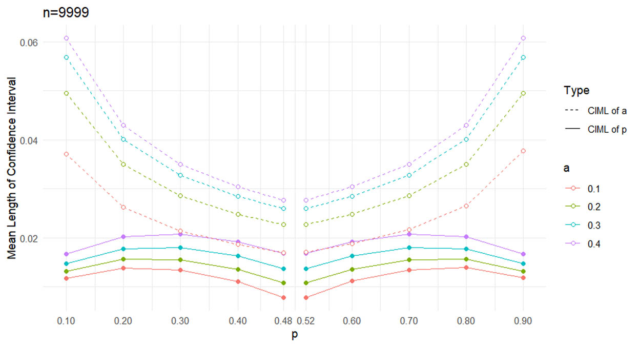
Furthermore, the results presented in Tables 3 and 4 demonstrate a noteworthy symmetry in the CIMLs when comparing parameter pairs equidistant from p = 0.5 for fixed a , i.e., for each fixed value of a , and for p values equidistant from p = 0.5 , the CIMLs for a and p are the same. Figure 1 shows this symmetry for n = 9,999 .

Figure 1

Symmetry in mean lengths of confidence intervals for “p” about p = 0.5 .

The observed behavior of the CIML for a and p can be explained by considering the variance-covariance matrix Σ − 1 from Theorem 6, which governs the precision of the MLEs a ˆ and p ˆ . When p is closer to 0.5, the off-diagonal elements (representing the covariance between a and p ) and the denominators in the variance terms become more influential. As p increases from 0.1 to 0.4 (for p < 0.5 ), the CIML for a decreases, indicating reduced uncertainty in estimating a due to lower variance. For p > 0.5 , as p moves further away from 0.5, the CIML for a increases again because of increased variance terms and covariance between a and p . The symmetry in the CIML for a around p = 0.5 (e.g., similar CIML for p = 0.1 and p = 0.9 ) suggests that confidence intervals widen as p deviates from 0.5 in either direction, reflecting greater difficulty in estimating a at extreme values of p .

For p , the mean length of the confidence intervals is relatively stable across different values, with small fluctuations likely due to the interaction between a and p in the variance terms of Σ − 1 . For small a (e.g., a = 0.1 ), the CIML for p is slightly lower when p is near 0.1 and 0.9 compared to intermediate values, indicating higher certainty in extreme probability scenarios. Given the large sample size ( n = 9,999 ), the confidence intervals are generally narrow, as the variance of the MLEs decreases with increasing sample size, leading to more precise estimates.

Overall, the behavior of the CIML for a and p reflects the interplay between the values of a and p , their interaction in the variance-covariance structure, and the large sample size ensuring narrow confidence intervals. The symmetry around p = 0.5 and the increasing interval lengths as p approaches the extremes illustrate the underlying statistical properties of the MLEs and their variances.

This symmetry reflects the underlying properties of the mixture copula model. The behavior suggests that the model treats the transition probabilities in a symmetric manner around p = 0.5 , ensuring that the statistical characteristics such as interval lengths and CPs remain stable for p values that are symmetrically opposite about 0.5. This property enhances the robustness of the parameter estimation process within the specified range of p .

5.2 Test for independence

5.2.1 Likelihood ratio test for independence

Tables 5 and 7 present the results of the likelihood ratio test for independence in the Markov chain generated by copula model (2.1) and Bernoulli( p ) marginal distribution. These tables provide separate results for p < 1 ⁄ 2 and p > 1 ⁄ 2 , respectively.

Table 5

Likelihood ratio test results

a	p	− 2 log Λ 1	Decision on H 0
0.1	0.1	1.9648	Fail to reject
0.1	0.2	75.3318	Reject
0.1	0.3	465.3507	Reject
0.1	0.4	1302.2148	Reject
0.2	0.1	62.5624	Reject
0.2	0.2	0.5426	Fail to reject
0.2	0.3	91.6928	Reject
0.2	0.4	537.1743	Reject
0.3	0.1	178.0430	Reject
0.3	0.2	85.5790	Reject
0.3	0.3	− 0.6683	Fail to reject
0.3	0.4	143.3914	Reject
0.4	0.1	315.6163	Reject
0.4	0.2	282.6401	Reject
0.4	0.3	93.5413	Reject
0.4	0.4	− 0.7403	Fail to reject
0.5	0.1	598.6498	Reject
0.5	0.2	678.1999	Reject
0.5	0.3	443.8051	Reject
0.5	0.4	175.6443	Reject
0.6	0.1	986.4705	Reject
0.6	0.2	1060.7808	Reject
0.6	0.3	908.5222	Reject
0.6	0.4	520.2437	Reject
0.7	0.1	1243.0918	Reject
0.7	0.2	1596.5124	Reject
0.7	0.3	1581.8311	Reject
0.7	0.4	1243.7897	Reject
0.8	0.1	1548.5890	Reject
0.8	0.2	2291.3934	Reject
0.8	0.3	2551.6879	Reject
0.8	0.4	2361.9013	Reject
0.9	0.1	2466.6171	Reject
0.9	0.2	3305.7161	Reject
0.9	0.3	3631.3346	Reject
0.9	0.4	3835.4538	Reject

Table 7

Likelihood ratio test results

a	p	− 2 log Λ 2	Decision on H 0
0.1	0.6	279.8288	Reject
0.1	0.7	107.8140	Reject
0.1	0.8	16.0485	Reject
0.1	0.9	0.3192	Fail to reject
0.2	0.6	111.3087	Reject
0.2	0.7	17.5196	Reject
0.2	0.8	0.4450	Fail to reject
0.2	0.9	12.1072	Reject
0.3	0.6	38.3697	Reject
0.3	0.7	− 1.3511	Fail to reject
0.3	0.8	15.9764	Reject
0.3	0.9	26.5985	Reject
0.4	0.6	0.0341	Fail to reject
0.4	0.7	17.6239	Reject
0.4	0.8	50.2535	Reject
0.4	0.9	62.1340	Reject
0.5	0.6	16.9398	Reject
0.5	0.7	97.3027	Reject
0.5	0.8	127.9626	Reject
0.5	0.9	165.1340	Reject
0.6	0.6	118.6838	Reject
0.6	0.7	195.6122	Reject
0.6	0.8	209.1521	Reject
0.6	0.9	222.3218	Reject
0.7	0.6	279.7745	Reject
0.7	0.7	328.9172	Reject
0.7	0.8	315.8419	Reject
0.7	0.9	263.6996	Reject
0.8	0.6	522.4635	Reject
0.8	0.7	557.5287	Reject
0.8	0.8	533.2392	Reject
0.8	0.9	284.6627	Reject
0.9	0.6	768.7074	Reject
0.9	0.7	688.8740	Reject
0.9	0.8	545.8894	Reject
0.9	0.9	411.5155	Reject

The Markov chain is generated using true values of a and p , and subsequently, a chi-squared independence test is performed based on the test statistics − 2 log Λ 1 and − 2 log Λ 2 , where Λ 1 and Λ 2 are given by formulae (4.3) and (4.4), respectively. A significance level of α = 0.05 is chosen for the test, implying that the null hypothesis of independence will be rejected if − 2 log Λ i ≥ 3.842 , i = 1 , 2 . Conversely, if − 2 log Λ i < 3.842 , the null hypothesis of independence is not rejected.

The chain is simulated for a total of n + 1 steps, where n is set to 9,999. The iterative process for Table 5 has true values of a ranging from 0.1 to 0.9 with a step of 0.1 and p < 1 ⁄ 2 ranging from 0.1 to 0.4 with a step of 0.1. On the other hand, Table 7 has true values of a ranging from 0.1 to 0.9 with a step of 0.1 and p > 1 ⁄ 2 ranging from 0.6 to 0.9 with a step of 0.1.

The test indicates that when a = p < 1 ⁄ 2 or a = 1 − p ≤ 1 ⁄ 2 , the Markov chain model generated by copula (2.1) and the Bernoulli( p ) marginal distribution transforms into independent Bernoulli trials.

5.2.2 Kolmogorov-Smirnov (KS) distance

We employed the KS distance to compare the copula of the sample with the independence copula. Specifically, we used it to test whether the empirical joint distribution of ( X t , X t + 1 ) deviates significantly from the product of their marginal distributions. The KS distance is given by

KS = sup x ∣ F ˆ ( X t , X t + 1 ) − F ˆ ( X t ) ⋅ F ˆ ( X t + 1 ) ∣ ,

where F ˆ ( X t , X t + 1 ) is the empirical joint distribution function of consecutive states, and F ˆ ( X t ) and F ˆ ( X t + 1 ) are the empirical marginal distribution functions of X t and X t + 1 , respectively.

A large KS distance suggests a significant departure from independence, indicating the presence of dependence in the Markov chain. The results of this test are summarized in Tables 6 and 8.

Table 6

KS distance values

a	p	KS distance	Decision on H 0
0.1	0.1	0.0027	Fail to reject
0.1	0.2	0.0181	Reject
0.1	0.3	0.0603	Reject
0.1	0.4	0.1188	Reject
0.2	0.1	0.0111	Reject
0.2	0.2	0.0009	Fail to reject
0.2	0.3	0.0297	Reject
0.2	0.4	0.0775	Reject
0.3	0.1	0.0203	Reject
0.3	0.2	0.0211	Reject
0.3	0.3	0.0013	Fail to reject
0.3	0.4	0.0433	Reject
0.4	0.1	0.0284	Reject
0.4	0.2	0.0403	Reject
0.4	0.3	0.0286	Reject
0.4	0.4	0.0020	Fail to reject
0.5	0.1	0.0379	Reject
0.5	0.2	0.0611	Reject
0.5	0.3	0.0617	Reject
0.5	0.4	0.0405	Reject
0.6	0.1	0.0507	Reject
0.6	0.2	0.0786	Reject
0.6	0.3	0.0887	Reject
0.6	0.4	0.0781	Reject
0.7	0.1	0.0606	Reject
0.7	0.2	0.0992	Reject
0.7	0.3	0.1177	Reject
0.7	0.4	0.1200	Reject
0.8	0.1	0.0701	Reject
0.8	0.2	0.1189	Reject
0.8	0.3	0.1510	Reject
0.8	0.4	0.1623	Reject
0.9	0.1	0.0916	Reject
0.9	0.2	0.1445	Reject
0.9	0.3	0.1718	Reject
0.9	0.4	0.1969	Reject

Table 8

KS distance values

a	p	KS distance	Decision on H 0
0.1	0.6	0.1188	Reject
0.1	0.7	0.0603	Reject
0.1	0.8	0.0181	Reject
0.1	0.9	0.0027	Fail to reject
0.2	0.6	0.0775	Reject
0.2	0.7	0.0297	Reject
0.2	0.8	0.0009	Fail to reject
0.2	0.9	0.0111	Reject
0.3	0.6	0.0433	Reject
0.3	0.7	0.0013	Fail to reject
0.3	0.8	0.0211	Reject
0.3	0.9	0.0203	Reject
0.4	0.6	0.0020	Fail to reject
0.4	0.7	0.0286	Reject
0.4	0.8	0.0403	Reject
0.4	0.9	0.0284	Reject
0.5	0.6	0.0365	Reject
0.5	0.7	0.0574	Reject
0.5	0.8	0.0559	Reject
0.5	0.9	0.0409	Reject
0.6	0.6	0.0781	Reject
0.6	0.7	0.0887	Reject
0.6	0.8	0.0786	Reject
0.6	0.9	0.0507	Reject
0.7	0.6	0.1200	Reject
0.7	0.7	0.1177	Reject
0.7	0.8	0.0992	Reject
0.7	0.9	0.0606	Reject
0.8	0.6	0.1623	Reject
0.8	0.7	0.1510	Reject
0.8	0.8	0.1189	Reject
0.8	0.9	0.0701	Reject
0.9	0.6	0.1969	Reject
0.9	0.7	0.1718	Reject
0.9	0.8	0.1445	Reject
0.9	0.9	0.0916	Reject

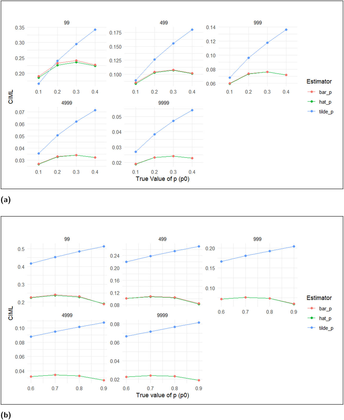
For this test, we defined the null hypothesis H 0 : the consecutive states in the Markov chain are independent, against the alternative hypothesis H 1 : the consecutive states exhibit some form of dependence. We conducted the test at a significance level of α = 0.05 for a sequence of length n = 9,999 . The test shows that when a = p < 1 2 or a = 1 − p ≤ 1 2 , the Markov chain model generated by copula (2.1) with Bernoulli( p ) marginals reduces to a sequence of independent Bernoulli trials.

5.3 Comparison of different estimators for the mean

This section is dedicated to the performance of the different estimators of the Bernoulli parameter. The MLEs are obtained numerically, and their confidence intervals are constructed. The sample mean satisfies the central limit theorem (9). The ( 1 − α ) 100 % confidence intervals for p are therefore

p ¯ ± z α ⁄ 2 p ¯ ( 1 − p ¯ ) n + 1 1 + a − 2 p ¯ 1 − a 1 ⁄ 2 , when p ¯ < 1 ⁄ 2 , p ¯ ± z α ⁄ 2 p ¯ ( 1 − p ¯ ) n + 1 a + 2 p ¯ − 1 1 − a 1 ⁄ 2 , when p ¯ ≥ 1 ⁄ 2 .

The other estimator for the mean ( p ) considered here is the robust estimator proposed by Longla and Peligrad [25]. It is based on a sample of dependent observations and requires some mild conditions to be satisfied on the variance of partial sums. The procedure is as follows: given the sample data ( X t ) 0 ≤ t ≤ n from a stationary sequence ( X t ) t ∈ Z , we generate another random sample ( Y t ) 0 ≤ t ≤ n independently of ( X t ) 0 ≤ t ≤ n and following a standard normal distribution. The Gaussian kernel and the optimal bandwidth h n are used. The optimal bandwidth, as proposed in Longla and Peligrad [25], for our case is

(5.1) h n = 1 ( n + 1 ) 2 1 ⁄ 5 .

To use this estimator, the following conditions must be satisfied (i.) ( X t ) t ∈ Z is an ergodic sequence, (ii.) ( X t ) t ∈ Z has finite second moments, and (iii.) ( n + 1 ) h n var ( p ¯ ) ⟶ 0 as n ⟶ ∞ . These conditions are easy to verify: (i.) the Markov chain X is ψ -mixing and hence ergodic. (ii.) The second condition follows from that V ar ( X 0 ) = p ( 1 − p ) < ∞ and E [ X 0 ] = p . (iii.) Using the variance of X ¯ given by (3.18), we see that

( n + 1 ) 1 ( n + 1 ) 2 1 ⁄ 5 p ( 1 − p ) ( n + 1 ) 1 + a − 2 p 1 − a + O ( 1 ⁄ n ) ⟶ 0 ,

as n ⟶ ∞ . The proposed robust estimator for the mean ( p ) of X is

p ˜ = 1 ( n + 1 ) h n ∑ t = 0 n X t exp − 1 2 Y t h n 2 .

A ( 1 − α ) 100 % confidence interval for p is

p ˜ 1 + h n 2 ± z α ⁄ 2 X ¯ n ( n + 1 ) 2 h n 1 ⁄ 2 .

Tables 9 and 10 present a comparison of the three estimators of p across varying true values of p . Samples of size n + 1 were utilized, and 95% confidence intervals were constructed. CPs were computed based on 400 replications of each of the chains of size n + 1 . Subsequently, the means of the lengths of the 400 confidence intervals were calculated to determine the confidence interval mean length. The results in both tables demonstrate that the estimators are asymptotically equivalent and converge to the true value. Note that we did not include the numerical values of the estimators because 400 numerical values were computed for each estimator in each case, and there is no criterion to choose only one representative from the 400. Relatively narrow confidence intervals reflect a higher level of precision in estimation, while wider confidence intervals indicate greater uncertainty in estimation.

Table 9

Comparison of the performance of p ˆ , p ¯ , and p ˜ for p < 0.5

n	Estimator	p 0
		0.1	0.2	0.3	0.4
99	p ˆ	CIML: 0.1862	CIML: 0.2258	CIML: 0.2355	CIML: 0.2245
		CP: 0.8625	CP: 0.9100	CP: 0.9275	CP: 0.9400
	p ¯	CIML: 0.1896	CIML: 0.2325	CIML: 0.2410	CIML: 0.2272
		CP: 0.9625	CP: 0.9475	CP: 0.9575	CP: 0.9625
	p ˜	CIML: 0.1656	CIML: 0.2399	CIML: 0.2946	CIML: 0.3416
		CP: 0.7875	CP: 0.9000	CP: 0.9325	CP: 0.9500
499	p ˆ	CIML: 0.0828	CIML: 0.1030	CIML: 0.1074	CIML:0.1012
		CP: 0.9050	CP: 0.9150	CP: 0.9450	CP: 0.9300
	p ¯	CIML: 0.0848	CIML: 0.1040	CIML: 0.1078	CIML:0.1016
		CP: 0.9450	CP: 0.9550	CP: 0.9375	CP: 0.9275
	p ˜	CIML: 0.0889	CIML: 0.1264	CIML: 0.1550	CIML: 0.1797
		CP: 0.8825	CP: 0.9325	CP: 0.9250	CP: 0.9675
999	p ˆ	CIML: 0.0591	CIML: 0.0732	CIML: 0.0761	CIML: 0.0717
		CP: 0.9375	CP: 0.9400	CP: 0.9375	CP: 0.9475
	p ¯	CIML: 0.0600	CIML: 0.0735	CIML: 0.0762	CIML: 0.0719
		CP: 0.9375	CP: 0.9700	CP: 0.9575	CP: 0.9550
	p ˜	CIML: 0.0678	CIML: 0.0962	CIML: 0.1179	CIML: 0.1362
		CP: 0.8825	CP: 0.9200	CP: 0.9300	CP: 0.9550
4,999	p ˆ	CIML: 0.0267	CIML: 0.0328	CIML: 0.0341	CIML: 0.0321
		CP: 0.9425	CP: 0.9575	CP: 0.9475	CP: 0.9350
	p ¯	CIML: 0.0268	CIML: 0.0329	CIML: 0.0341	CIML: 0.0321
		CP: 0.9625	CP: 0.9600	CP: 0.9400	CP: 0.9525
	p ˜	CIML:0.0356	CIML: 0.0505	CIML: 0.0619	CIML: 0.0716
		CP: 0.9000	CP: 0.9200	CP: 0.9425	CP: 0.9450
9,999	p ˆ	CIML: 0.0189	CIML: 0.0232	CIML: 0.0241	CIML: 0.0227
		CP: 0.9525	CP: 0.9550	CP: 0.9500	CP: 0.9300
	p ¯	CIML: 0.0190	CIML: 0.0232	CIML: 0.0241	CIML: 0.0227
		CP: 0.9500	CP: 0.9570	CP: 0.9625	CP: 0.9450
	p ˜	CIML: 0.0270	CIML: 0.0383	CIML: 0.0470	CIML: 0.0542
		CP: 0.9025	CP: 0.9000	CP: 0.9500	CP: 0.9500

A fixed value of a = 0.5 was used in all the cases, and 95% confidence intervals were constructed. Est denotes the estimator and p 0 denotes the true value of p .

Table 10

Comparison of the performance of p ˆ , p ¯ and p ˜ for p ≥ 0.5

n	Estimator	p 0
		0.6	0.7	0.8	0.9
99	p ˆ	CIML: 0.2242	CIML: 0.2381	CIML: 0.2286	CIML: 0.1912
		CP: 0.9575	CP: 0.9275	CP: 0.9250	CP: 0.8900
	p ¯	CIML: 0.2272	CIML: 0.2410	CIML: 0.2326	CIML: 0.1896
		CP: 0.9450	CP: 0.9575	CP: 0.9450	CP: 0.9500
	p ˜	CIML: 0.4163	CIML: 0.4529	CIML: 0.4841	CIML: 0.5124
		CP: 0.9450	CP: 0.9525	CP: 0.9575	CP: 0.9700
499	p ˆ	CIML: 0.1013	CIML: 0.1071	CIML: 0.1032	CIML: 0.0832
		CP: 0.9200	CP: 0.9425	CP: 0.9550	CP: 0.9075
	p ¯	CIML: 0.1016	CIML: 0.1077	CIML: 0.1040	CIML: 0.0848
		CP: 0.9575	CP: 0.9475	CP: 0.9475	CP: 0.9400
	p ˜	CIML: 0.2200	CIML: 0.2381	CIML: 0.2543	CIML: 0.2695
		CP: 0.9450	CP: 0.9650	CP: 0.9500	CP: 0.9775
999	p ˆ	CIML: 0.0716	CIML: 0.0759	CIML: 0.0731	CIML: 0.0595
		CP: 0.9275	CP: 0.9175	CP: 0.9400	CP: 0.9225
	p ¯	CIML: 0.0719	CIML: 0.0762	CIML: 0.0735	CIML: 0.0600
		CP: 0.9475	CP: 0.9350	CP: 0.9625	CP: 0.9175
	p ˜	CIML: 0.1664	CIML: 0.1803	CIML: 0.1926	CIML: 0.2042
		CP: 0.9525	CP: 0.9725	CP: 0.9550	CP: 0.9375
4,999	p ˆ	CIML: 0.0321	CIML: 0.0341	CIML: 0.0329	CIML: 0.0268
		CP: 0.9400	CP: 0.9425	CP: 0.9500	CP: 0.9400
	p ¯	CIML: 0.0321	CIML: 0.0341	CIML: 0.0329	CIML: 0.0268
		CP: 0.9550	CP: 0.9275	CP: 0.9525	CP: 0.9625
	p ˜	CIML: 0.0876	CIML: 0.0946	CIML: 0.1012	CIML: 0.1073
		CP: 0.9475	CP: 0.9525	CP: 0.9500	CP: 0.9525
9,999	p ˆ	CIML: 0.0227	CIML: 0.0241	CIML: 0.0233	CIML: 0.0190
		CP: 0.9500	CP: 0.9500	CP: 0.9475	CP: 0.9425
	p ¯	CIML: 0.0227	CIML: 0.0241	CIML: 0.0233	CIML: 0.0190
		CP: 0.9500	CP: 0.9450	CP: 0.9450	CP: 0.9500
	p ˜	CIML: 0.0664	CIML: 0.0717	CIML: 0.0767	CIML: 0.0813
		CP: 0.9700	CP: 0.9725	CP: 0.9700	CP: 0.9650

A fixed value a = 0.5 was used in all the cases, and 95% confidence intervals were constructed. Est denotes the estimator, and p 0 denotes the true value of p .

In both cases of p < 1 ⁄ 2 and p > 1 ⁄ 2 , p ˆ yields the most precise estimates with the shortest mean confidence intervals. The sample mean closely follows p ˆ in precision but exhibits slightly longer mean confidence intervals. Although the robust estimator shows larger mean confidence intervals compared to p ˆ and p ¯ , it still provides reasonable estimates, especially with larger sample sizes. This comparison is presented on the plots in Figure 2(a) and (b).

$Figure 2 CIML for different values of p p : (a) CIML for estimators when p < 1 2 p\lt \frac{1}{2} and (b) CIML for estimators when p > 1 2 p\gt \frac{1}{2} .$

Figure 2

CIML for different values of p : (a) CIML for estimators when p < 1 2 and (b) CIML for estimators when p > 1 2 .

Both the MLE and the robust estimator demonstrate sensitivity to sample size, resulting in initially low CPs. However, as the sample size increases, these probabilities approach the desired 95% level. The CPs for the sample mean ( p ¯ ) consistently approach the desired nominal level, indicating reliable confidence intervals across different sample sizes.

The performance of the robust estimator is less optimal with smaller sample sizes but improves as the sample size increases. The robust estimator is designed to be competitive in data containing noise or outliers; however, the data considered here has neither.

While all three estimators provide asymptotically unbiased estimates for the Bernoulli parameter p , the sample mean ( p ¯ ) generally strikes the best balance between precision and accuracy, making it the preferred choice for estimating p in this context.

6 Conclusion

The mixing properties of copula-based Markov chains are highly dependent on the chosen marginal distributions. Some copulas that do not generate mixing with continuous marginals may generate mixing with discrete marginals, so generalizations should be approached with caution. In this article, we have demonstrated that copulas from the Fréchet (Mardia) family generate ψ -mixing Markov chains for a + b = 1 , which is not the case when the marginals are uniform [ 0 , 1 ] . Understanding these mixing properties is crucial for deriving central limit theorems for sample means, which in turn facilitates the construction of confidence intervals for the sample means based on the standard normal distribution.

Acknowledgments

The authors would like to thank the reviewers for their valuable comments and suggestions, which have greatly contributed to improving this work.

Funding information: The authors state no funding involved.
Author contributions: All authors share full responsibility for the content of this manuscript. They have jointly agreed to its submission, carefully examined the results, and approved the final version for publication.
Conflict of interest: The authors state no conflict of interest.

References

[1] Anderson, W., & Goodman, A. (1957). Statistical inference about Markov chains. The Annals of Mathematical Statistics, 28, 89–110. 10.1214/aoms/1177707039Search in Google Scholar

[2] Bedrick, J., & Aragon, J. (1989). Approximate confidence intervals for the parameters of a stationary binary Markov chain. Technometrics, 31, 437–448. 10.1080/00401706.1989.10488592Search in Google Scholar

[3] Billingsley, P. (1961). Statistical methods in Markov chains. The Annals of Mathematical Statistics, 32, 12–40. 10.1214/aoms/1177705136Search in Google Scholar

[4] Billingsley, P. (1961). Statistical Inference for Markov Processes. Institute of Mathematical Statistics-University of Chicago Statistical Research Monographs, Chicago: University of Chicago Press. Search in Google Scholar

[5] Blum, R., Hanson, L., & Koopmans, L. (1963). On the strong law of large numbers for a class of stochastic processes. Albuquerque, NM: Sandia Corporation. 10.1007/BF00535293Search in Google Scholar

[6] Bradley, R. (2007). Introduction to strong mixing conditions (vol. 1, 2), Kendrick Press. Search in Google Scholar

[7] Brainerd, B., & Chang, M. (1982). Number of occurrences in two-state Markov chains, with applications in linguistics. The Canadian Journal of Statistics, 10, 225–231. 10.2307/3556186Search in Google Scholar

[8] Cogburn, R. (1960). Asymptotic properties of stationary sequences (Vol. 3), Berkeley, CA: University of California Press. Search in Google Scholar

[9] Crow, E. (1979). Approximate confidence intervals for a proportion from Markov dependent trials. Communications in Statistics, Part B-Simulation and Computation, 8, 1–24. 10.1080/03610917908812101Search in Google Scholar

[10] David, F. (1947). A power function for tests of randomness in a sequence of alternatives. Biometrika, 34, 335–339. 10.1093/biomet/34.3-4.335Search in Google Scholar

[11] Darsow, F., Nguyen, B., & Olsen, E. (1992). Copulas and Markov processes. Illinois Journal of Mathematics, 36(4), 600–642. 10.1215/ijm/1255987328Search in Google Scholar

[12] Durante, F., & Sempi, C. (2015). Principles of copula theory. Boca Raton, FL: CRC Press. 10.1201/b18674Search in Google Scholar

[13] Goodman, A. (1958). Simplified run tests and likelihood ratio tests for Markoff chains. Biometrika, 45(1/2), 181–197. 10.1093/biomet/45.1-2.181Search in Google Scholar

[14] Goodman, A. (1959). On some statistical tests for mth order Markov chains, Ann. Math. Statist. 30, 154–164. 10.1214/aoms/1177706368Search in Google Scholar

[15] Ibragimov, A. (1959). Some limit theorems for stochastic processes stationary in the strict sense. Dokl. Akad. Nauk SSSR, 125, 711–714. Search in Google Scholar

[16] Ibragimov, A., & Linnik, V. (1975). Independent and stationary sequences of random processes, Wolters: Nordhoff Publications. Search in Google Scholar

[17] Joe, H. (1997). Multivariate models and multivariate dependence concepts. Boca Raton, FL: CRC Press. 10.1201/b13150Search in Google Scholar

[18] Johnson, C., & Klotz, J. (1974). The atom probe and Markov chain statistics of clustering. Technometrics, 16, 483–493. 10.1080/00401706.1974.10489229Search in Google Scholar

[19] Klotz, J. (1972). Markov chain clustering of births by sex. Proc. Sixth Berkeley Symp. Math. Statist. Prob (vol. 4, pp. 173–185), Berkeley, CA: University of California Press. 10.1525/9780520422001-016Search in Google Scholar

[20] Klotz, J. (1973). Statistical inference in Bernoulli trials with dependence. Annals of Statistics, 1, 373–379. 10.1214/aos/1176342377Search in Google Scholar

[21] Lindqvist, B. (1976). A note on Bernoulli trials with dependence, Scandinavian Journal of Statistics, 5, 205–208. Search in Google Scholar

[22] Longla, M., & Peligrad, M. (2012). Some aspects of modeling dependence in copula based Markov chains. Journal of Multivariate Analysis, 111, 234–240. 10.1016/j.jmva.2012.01.025Search in Google Scholar

[23] Longla, M. (2014). On Dependence Structure of Copula-based Markov Chains. ESAIM: Probability and Statistics, 18, 570–583, DOI: 10.1051/ps/2013052. Search in Google Scholar

[24] Longla, M. (2015). On mixtures of copulas and mixing coefficients. Journal of Multivariate Analysis, 139, 259–265. 10.1016/j.jmva.2015.03.009Search in Google Scholar

[25] Longla, M., & Peligrad, M. (2021). New robust confidence intervals for mean under dependence, Journal of Statistics Planning and Inference, 211, 90–106. 10.1016/j.jspi.2020.06.001Search in Google Scholar

[26] Muia, M. (2024). Dependence and Mixing for Perturbations of Copula-based Markov Chains, Ph.D. thesis, ProQuest, Ann Arbor, MI: University of Mississippi. Search in Google Scholar

[27] Nelsen, R. (2006). Introduction to Copulas. Springer Series in Statistics (2nd ed.), New York: Springer-Verlag. Search in Google Scholar

[28] Philipp, W. (1969). The central limit problem for mixing sequences of random variables. Zeitschrift für Wahrscheinlichkeitstheorie und verwandte Gebiete, 12(2), 155–171. 10.1007/BF00531648Search in Google Scholar

[29] Price, B. (1976). A note on estimation in Bernoulli trials with dependence. Communication in Statistics, Part A-Theory and Methods, 5, 661–671. 10.1080/03610927608827383Search in Google Scholar

[30] Sklar, A. (1959). Fonctions de repartition an dimensions et leurs marges (vol. 8, pp. 119–231), Paris: Publ. inst. statist. University. Search in Google Scholar

[31] Wilks, S. (1938). The large sample distribution of the likelihood ratio for testing com posite hypothese. Ann. Math. Stat. 9, 60–62. 10.1214/aoms/1177732360Search in Google Scholar

Received: 2024-10-19

Revised: 2025-05-11

Accepted: 2025-06-29

Published Online: 2025-08-13

This work is licensed under the Creative Commons Attribution 4.0 International License.

Articles in the same Issue

https://doi.org/10.1515/demo-2025-0015

Keywords for this article

asymptotic normality; dependent Bernoulli trials; Frechet family of copulas; mixing for Markov chains

Creative Commons

BY 4.0