On bivariate Archimedean copulas with fractal support
-
Juan Fernández Sánchez


Abstract
Due to their simple analytic form (bivariate) Archimedean copulas are usually viewed as very smooth and handy objects, which should distribute mass in a fairly regular and certainly not in a pathological way. Building upon recently established results on the Archimedean family and working with iterated function systems with probabilities, we falsify this natural conjecture and derive the surprising result that for every
1 Introduction
Considering Lipschitz continuity and the fact that bivariate copulas are distributions functions (restricted to [0, 1]2) of random vectors
Since then various papers on copulas with fractal support have appeared in the literature, each of them underlining the fact that analytically nice objects (Lipschitz continuous, common marginals, etc.) like copulas may exhibit surprisingly irregular/pathological analytic behavior: In [28], we showed that the result by Fredricks et al. also holds for the subclass of the so-called idempotent copulas (idempotent with respect to the star-product going back to Darsow et al. in [7] and corresponding to the standard composition of transition probabilities well known from the Markov chain setting) and generalized the IFS construction to arbitrary dimensions
While each of the afore-mentioned contributions illustrates that the family
The remainder of this note is organized as follows: Section 2 gathers notation and preliminaries, Section 3 presents some auxiliary results on Cantor functions needed in the sequel. All main results are presented in Section 4. Several graphics and an example corresponding to the classical middle third Cantor set illustrate the chosen procedures and underlying ideas.
2 Notation and preliminaries
For every metric space
As already mentioned,
A Markov kernel from
holds for
As a special case, the latter yields that
holds for every
Archimedean copulas can be expressed via generators
To simplify notation in what follows, we will work with the convention
to which we will refer as the (strict or nonstrict) Archimedean copula induced by
In what follows, we will let
According to [24] for every Archimedean copula
have that
for every
Before providing an explicit expression of the Markov kernel of a general (nonstrict) Archimedean copula, we first recall some analytic properties of generators that will be used in the sequel: For every generator
To simplify notation, for every
is a Markov kernel of
Moreover we have
As shown in [13,24], the Kendall distribution function
We will directly use these expressions in the next sections in order to show that the probability measure
Remark 2.1
Our construction of Archimedean copulas with fractal support in Section 4 is based on nonstrict generators, which are continuously differentiable, so the (two-sided) derivative
Keeping notation simple, for (continuously) differentiable generators
is continuous on
As a last key component, we recall the definition of an IFS and some main results about IFSs [5,11,12,21]. Suppose for the following that
It can be shown [5,12,21] that
The attractor
An IFS together with a vector
The so-called Hutchison metric
where
The fixed point
Attractors of IFSs are strongly interrelated with symbolical dynamical systems via the so-called address map [5,21]: For every
To simplify notation in what follows, we will write
it is straightforward to verify that
Suppose now that
then [21]
and extending in the standard way to full
3 Auxiliary results on Cantor functions
Since for the construction of Archimedean copulas with fractal support, we will work with Cantor functions, we recall their construction via IFSs (only consisting of two functions) and then derive some properties needed in the sequel. For every
set
Obviously
holds. Defining
with
Note that by using the Hutchinson operator, we obviously have
Considering that the IFSP construction of
For confirming that the function
which either follows geometrically by using symmetry (the endo- and the hypergraph of
implying
Example 3.1
For the case
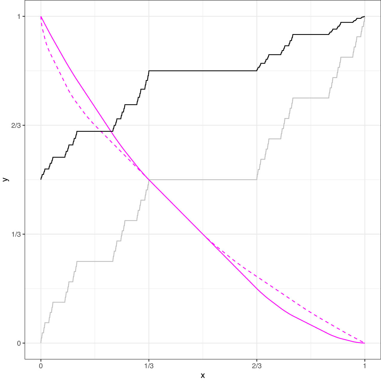
Approximation of the classical (middle third) Cantor function
4 Constructing bivariate Archimedean copulas with fractal support
Let
Then obviously we have
Letting
i.e., the copula
for every
![Figure 2
3D-plot of (an approximation of) the copula
A
r
0
{A}_{{r}_{0}}
considered in Examples 3.1 and 4.3; the lines depict the graphs of the function
f
t
{f}^{t}
with
t
∈
0
,
1
6
,
1
3
,
1
2
,
2
3
,
5
6
t\in \left\{\phantom{\rule[-0.95em]{}{0ex}},0,\frac{1}{6},\frac{1}{3},\frac{1}{2},\frac{2}{3},\frac{5}{6}\right\}
.](/document/doi/10.1515/demo-2025-0013/asset/graphic/j_demo-2025-0013_fig_002.jpg)
3D-plot of (an approximation of) the copula
We are now going to show that the Hausdorff dimension of the support of
for every interval
Lemma 4.1
Letting
Proof
Notice that each of the intervals
Having this, using
Lemma 4.2
The support
Moreover, the support of the probability measure
Proof
Considering that
Considering
follows, which directly yields
(ii) For sufficiently small
Continuity of
Considering that
(í) Proceeding in the same manner shows that for every
Since the set
which completes the proof of the first assertion. The second assertion follows from equivalence (18).□
Example 4.3
For the case
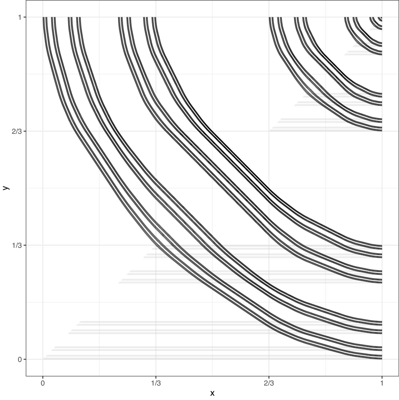
Approximation of the support of the copula
Lemma 4.4
The support
Proof
We will use the fact that bi-Lipschitz transformtions [12] preserve the Hausdorff dimension and proceed as follows: Define the sets
Then proceeding as with the support of
obviously
for every
Using countable stability of the Hausdorff dimension (again see [12]) therefore yields
Having that, considering that both the sets
which completes the proof.□
Summing up, we can finally formulate and prove our main result:
Theorem 4.5
For every
Proof
Considering the fact that the aforementioned mapping
Remark 4.6
Recently established results focusing on the interplay of Archimedean copulas and the so-called Williamson measures [19] allow for alternative ways to construct Archimedean copulas with fractal support. One may, for instance, start with the classical Cantor measure
Acknowledgments
The second author gratefully acknowledges the support of the WISS 2025 project ‘IDA-lab Salzburg’ (20204-WISS/225/197-2019 and 20102-F1901166-KZP).
-
Author contributions: Both authors have accepted responsibility for the entire content of this manuscript and consented to its submission to the journal, reviewed all the results, and approved the final version of the manuscript. JFS: conceptualization and methodology. WT: conceptualization, methodology, and writing.
-
Conflict of interest: The authors state no conflict of interest.
-
Data availability statement: Data sharing is not applicable to this article as no datasets were generated or analysed during the current study.
References
[1] de Amo, E., Díaz Carrillo, M., & Fernández-Sánchez, J. (2011). Measure-Preserving Functions and the Independence Copula. Mediterr. J. Math. 8, 431–450, DOI: https://doi.org/10.1007/s00009-010-0073-9. 10.1007/s00009-010-0073-9Search in Google Scholar
[2] de Amo, E., Díaz Carrillo, M., & Fernández-Sánchez, J. (2012). Copulas and associated fractal sets. Journal of Mathematical Analysis and Applications, 386, 528–541, DOI: https://doi.org/10.1016/j.jmaa.2011.08.017. 10.1016/j.jmaa.2011.08.017Search in Google Scholar
[3] de Amo, E., Díaz Carrillo, M., Fernández-Sánchez, J., & Salmerón, A. (2012). Moments and associated measures of copulas with fractal support. Applied Mathematics and Computation, 218, 8634–8644, DOI: https://doi.org/10.1016/j.amc.2012.02.025. 10.1016/j.amc.2012.02.025Search in Google Scholar
[4] De Amo, E., Díaz Carrillo, M., Fernández-Sánchez, J., & Trutschnig, W. (2013). Some results on homeomorphisms between fractal supports of copulas. Nonlinear Anal-Theor, 85, 132–144, DOI: https://doi.org/10.1016/j.na.2013.02.027. 10.1016/j.na.2013.02.027Search in Google Scholar
[5] Barnsley, M. F. (1993). Fractals everywhere. Cambridge: Academic Press. Search in Google Scholar
[6] Bishop, C. J., & Peres, Y. (2016). Fractals in Probability and Analysis. Cambridge: Cambridge University Press. 10.1017/9781316460238Search in Google Scholar
[7] Darsow, W. F., Nguyen, B., & Olsen, E. T. (1992). Copulas and Markov processes. Illinois Journal of Mathematics, 36, 600–642. https://api.semanticscholar.org/CorpusID:119359664. 10.1215/ijm/1255987328Search in Google Scholar
[8] Dudley, R. M. (2002). Real Analysis and Probability. Cambridge: Cambridge University Press. 10.1017/CBO9780511755347Search in Google Scholar
[9] Durante, F., & Sempi, C. (2015). Principles of Copula Theory. Chapman and Hall/CRC. 10.1201/b18674Search in Google Scholar
[10] Durante, F., Fernández Sánchez, J., & Trutschnig, W. (2020). Spatially homogeneous copulas. Annals of the Institute of Statistical Mathematics, 72, 607–626, DOI: https://doi.org/10.1007/s10463-018-0703-8. 10.1007/s10463-018-0703-8Search in Google Scholar
[11] Edgar, G. A. (1990). Measure, Topology and Fractal Geometry. Heidelberg New York: Springer Berlin. 10.1007/978-1-4757-4134-6Search in Google Scholar
[12] Falconer, K. (2003). Fractal Geometry, Mathematical Foundations and Applications, 2nd Edition, New York and London: John Wiley and Sons. 10.1002/0470013850Search in Google Scholar
[13] Fernández Sánchez, J., & Trutschnig, W. (2015). Singularity aspects of Archimedean copulas. Journal of Mathematical Analysis and Applications, 432, 103–113, DOI: https://doi.org/10.1016/j.jmaa.2015.06.036. 10.1016/j.jmaa.2015.06.036Search in Google Scholar
[14] Fernández Sánchez, J., & Trutschnig, W. (2023). A link between Kendallas tau, the length measure and the surface of bivariate copulas, and a consequence to copulas with self-similar support. Dependence Model, 11, 20230105, DOI: https://doi.org/10.1515/demo-2023-0105. 10.1515/demo-2023-0105Search in Google Scholar
[15] Fredricks, G., Nelsen, R., & Rodríguez-Lallena, J. A. (2005). Copulas with fractal supports. Insurance: Mathematics and Economics, 37, 42–48, DOI: https://doi.org/10.1016/j.insmatheco.2004.12.004. 10.1016/j.insmatheco.2004.12.004Search in Google Scholar
[16] Hatano, K. (1971). Notes on Hausdorff dimensions of Cartesian product sets. Hiroshima Mathematical Journal, 1, 17–25, DOI: https://doi.org/10.32917/hmj/1206138139. 10.32917/hmj/1206138139Search in Google Scholar
[17] Kallenberg, O. (1997). Foundations of modern probability. New York Berlin Heidelberg: Springer Verlag. Search in Google Scholar
[18] Kannan, R., & Krueger, C. K. (1996). Advanced analysis on the real line. New York: Springer Verlag. Search in Google Scholar
[19] Kasper, T., Dietrich, N., & Trutschnig, W. (2024). On convergence and mass distributions ofmultivariate Archimedean copulas and their interplay with the Williamson transform. Journal of Mathematical Analysis and Applications, 529, 127555, DOI: https://doi.org/10.1016/j.jmaa.2023.127555. 10.1016/j.jmaa.2023.127555Search in Google Scholar
[20] Klenke, A. (2007). Probability Theory - A Comprehensive Course. Berlin Heidelberg: Springer Verlag. Search in Google Scholar
[21] Kunze, H., LaTorre, D., Mendivil, F., & Vrscay, E. R. (2012). Fractal Based Methods in Analysis. New York Dordrecht Heidelberg London: Springer. 10.1007/978-1-4614-1891-7Search in Google Scholar
[22] McNeil, A., & Nešlehová, J. (2009). Multivariate Archimedean Copulas, d-monotone functions and ℓ1-norm symmetric distributions. Annals of Statistics, 37, 3059–3097, DOI: https://doi.org/10.1214/07-AOS556. 10.1214/07-AOS556Search in Google Scholar
[23] Mai, J. F., & Scherer, M. (2011). Bivariate extreme-value copulas with discrete Pickands dependence measures. Extreme, 14, 311–324, DOI: https://doi.org/10.1007/s10687-010-0112-8. 10.1007/s10687-010-0112-8Search in Google Scholar
[24] Nelsen, R. B. (2006). An Introduction to Copulas. New York: Springer Series in Statistics. Search in Google Scholar
[25] Pollard, D. (2001). A Useras Guide to Measure Theoretic Probability. Cambridge: Cambridge University Press. 10.1017/CBO9780511811555Search in Google Scholar
[26] Rudin, W. (1966). Real and Complex Analysis. New York: McGraw-Hill. Search in Google Scholar
[27] Trutschnig, W. (2011). On a strong metric on the space of copulas and its induced dependence measure. Journal of Mathematical Analysis and Applications, 384, 690–705, DOI: https://doi.org/10.1016/j.jmaa.2011.06.013. 10.1016/j.jmaa.2011.06.013Search in Google Scholar
[28] Trutschnig, W., & Fernández-Sánchez, J. (2012). Idempotent and multivariate copulas with fractal support. Journal of Statistical Planning and Inference, 142, 3086–3096, DOI: https://doi.org/10.1016/j.jspi.2012.06.012. 10.1016/j.jspi.2012.06.012Search in Google Scholar
[29] Trutschnig, W., Schreyer, M., & Fernández-Sánchez, J. (2016). Mass distributions of two-dimensional extreme-value copulas and related results. Extremes, 19, 405–427, DOI: https://doi.org/10.1007/s10687-016-0249-1. 10.1007/s10687-016-0249-1Search in Google Scholar
© 2025 the author(s), published by De Gruyter
This work is licensed under the Creative Commons Attribution 4.0 International License.
Articles in the same Issue
- Research Articles
- Tree-based conditional copula estimation
- Fast estimation of Kendall's Tau and conditional Kendall's Tau matrices under structural assumptions
- On bivariate Archimedean copulas with fractal support
- A point on discrete versus continuous state-space Markov chains
- Dependence modeling in general insurance using local Gaussian correlations and hidden Markov models
- Review Article
- Generalized Hoeffding-Fréchet functionals and mass transportation