Dependence modeling in general insurance using local Gaussian correlations and hidden Markov models
-
Zabibu Afazali


Abstract
This article introduces a hybrid framework that combines local Gaussian correlation (LGC) with hidden Markov models (HMMs) to model dynamic and nonlinear dependencies in general insurance claims, thereby addressing the limitations of static copula methods. When applied to Kenyan motor insurance claims (2008–2021) and Norwegian home insurance data (2012–2018), the proposed LGC-HMM approach captures regime-specific, nonlinear dependency patterns, revealing distinct stable and crisis periods through structural breaks in the dependency structure. Diagnostic checks confirm the HMM’s ability to reduce residual serial dependence, validating the latent state dynamics. Regime-aware value-at-risk (VaR) and tail VaR estimates derived from the LGC-HMM, using a proposed simulation procedure, outperform static copula models by adapting to structural changes, demonstrating robust forecasting performance. Visualization of forecasts via LGC maps further illustrates evolving tail dependencies. These findings support improved risk diversification and crisis-sensitive pricing strategies in actuarial practice.
1 Introduction
Risk assessment and estimating claim dependencies are paramount for effective pricing, reserving, and risk management in the insurance industry. Various recent methods and techniques have been developed for modeling insurance claim dependencies. Based on the findings of Cossette et al. [14], Bolance et al. [10], Bolané et al. [9], it is apparent that a robust dependence modeling framework is essential for determining the allocation of risk capital to each line of business (LoB) or business segments. Copula-based models have become increasingly popular when modeling the dependence of insurance claims. Among the prominent works in this field is Joe [26], where copulas were applied to model the tail dependence between large insurance losses. It was found that assessing risks accurately requires capturing extreme dependence structures. Further advancements in copula-based approaches include the work of Embrechts et al. [16], who introduced the concept of Archimedean copulas to model dependence in insurance portfolios. Their findings demonstrated the suitability of Archimedean copulas in capturing tail dependencies, allowing for better risk assessment and diversification analysis. Diers et al. [15] used the Bernstein copula to model dependencies between six insurance LoBs, and MFarri and Moutanabbir [32] used a mixed Bernstein copula, which represents a generalization of the well-known Archimedean copulas. The Bernstein Copula is flexible in mapping in-homogeneous dependence structures and can approximate any copula arbitrarily well. Previous studies [15,40] noted that akin to other nonparametric estimators, the Bernstein copula suffers from drawbacks, including bias-variance trade-off and the inability to model asymptotic tail dependence.
To date, insurers understand that diversification is at the foundation of the insurance business, and as such, developing tools and motivations to enable them to understand the value of dependency modeling is an important research area in the field of insurance and statistics [19]. Copula models, while frequently employed for depicting dependency structures, typically entail only a single parameter, which can be challenging to interpret. Their methodology for gauging dependence is often rudimentary, relying on simulated observations and subsequent examination of scatter diagrams, which inadequately quantifies dependence [6].
Alexeev et al. [1] noted that one of the primary objectives of general insurance providers is to assess the total risk associated with a portfolio of losses when LoBs are correlated. Their research provides valuable insight into the dependency between insurance LoBs using copula functions and skewed generalized hyperbolic marginal distributions. In their study and many others, such as Lane [29] and Vernic [47], they observed that the data were still positively skewed even after a logarithmic transformation. Nevertheless, in practice, some regulatory requirements, such as Solvency II, still propose a log-normal distribution for losses in the standard formula for solvency capital requirement [41]. These findings necessitate an excellent alternative approach to model dependence structure, and one possibility is the local Gaussian correlation (LGC) [45], whose advantages are in its flexibility, ease of application, and interpretation, whose methodology is presented in more detail in Section 2. The local Gaussian correlation (LGC) expands Gaussian analysis to nonlinear settings while retaining standard correlation interpretations. Moreover, it offers an efficient means to estimate and visually represent dependency structures. In addition, the LGC enables describing the dependence structure through localized correlation estimates.
In formulating the LGC formula, local approximations of bivariate Gaussian densities are achieved through likelihood estimation employing a bivariate correlation function. Each data point encompasses the correlation coefficient characterizing the local Gaussian approximation. The LGC employs a Gaussian kernel, serving as a smoothing mechanism that assigns weights to neighboring data points proportionate to their proximity to the central point. Weightage diminishes with increasing distance from the central point, ensuring that distant data points exert lesser influence on the resultant estimation [37]. In addition, we introduce a novel approach for modeling time-varying dependence in claim payouts by integrating the LGC with hidden Markov models (HMMs). Gundersen et al. [22] applied this method in financial markets, demonstrating that bear market regimes exhibit reduced yet asymmetric dependence, indicating the loss of diversification benefits during crisis periods. We introduce the application of their methodology to modeling dependencies in insurance portfolio.
Insurance claim data provides a dynamic narrative of events and interactions, providing a valuable source of sequential information. For insurers to mitigate financial volatility and assess risks accurately, capturing time dependencies in claim payout data is essential. As such, Araichi et al. [2] used the generalized autoregressive conditional sinistrality model to analyze the evolution of time-dependent relationships and used a copula function to aggregate risks over time. The study by Oflaz [36] found that a diversification effect could be gained on solvency capital when time-varying dependence models are used. The integration of LGC with HMM offers an alternative novel approach to capture time-varying dependence in claim payouts. We employ a hybrid modeling framework that combines HMMs with LGC to capture both the latent regime-switching behavior and the nonlinear, time-varying dependence structures observed in insurance claims data. While HMMs are powerful for detecting structural breaks and modeling unobserved change points caused by external shocks such as the COVID-19 pandemic or political instability [12,34], they typically rely on assumptions about dependence (e.g., constant or linear correlations) that may not hold in real-world insurance applications [23,49]. To overcome this limitation, we incorporate LGC, a flexible and fully nonparametric measure of dependence that captures local features of the joint distribution, including asymmetries and tail dependencies, without imposing global constraints like linearity or elliptical copulas [38,45]. This is especially important in the context of multivariate insurance claims, where dependence between lines of business can evolve not only across regimes, but also within regimes, in response to subtle changes in the economic environment, policyholder behavior, or market conditions. By combining HMMs and LGC, our model offers a robust and interpretable framework for uncovering hidden states while simultaneously capturing the fine-grained, time-local dependence structures that classical time series and copula-based models tend to overlook [13,30]. This dual-layer approach enhances the model’s ability to provide early warnings and regime-specific risk insights, which are critical for actuarial decision-making and regulatory response.
This article’s results are critical for understanding temporal dependencies in insurance claim data, as highlighted by Araichi et al. [2] who used Copulas. This enables more accurate risk assessment and empowers insurers to adapt strategies that mitigate financial volatility, and realize diversification benefits, even during times of crisis in financial markets. For application to risk management in insurance, our study goes further to compare our approach with copula-based models by estimating value at risk (VaR). In recent studies, researchers Ghosh et al. [20] and Diers et al. [15] have shown that using copulas is effective for modeling the relationship between insurance claims and for calculating VaR. We generated observations from the LGC density and calculated VaRs, comparing them with VaRs obtained from selected copulas, including the independence copula.
The article’s subsequent sections are organized as follows: Section 2 provides an overview of the Methods and Materials, detailing the application of LGC for dependence modeling and the integration of HMMs to capture potential time-varying dependencies. It also elaborates on using LGC to test for independence between claims payout of insurance LoBs and examine differences in dependence structures across regimes. We furthermore present a novel simulation technique from the LGC density in this section, while Section 2.5 comprehensively describes the datasets utilized in the analysis. Section 3 presents the results, discussion, and visualizations of the prevailing dependence structures and HMM time series plots. In Section 3.3, we provide a risk modeling application by comparing VaRs estimates from LGC model and well-known copula models. Finally, Section 4 presents a discussion and some concluding remarks, underscoring the importance of understanding and modeling dependencies between insurance claim types for effective risk management. In this article, we use the words “state” and “regime” interchangeably.
2 Materials and methods
2.1 LGC
Let
where
The density
The variables themselves are not required to follow a Gaussian distribution, as the local Gaussian approach will approximate a specific region of the dataset to adhere to Gaussian density characteristics. Thus, LGC provides a localized Gaussian approximation that captures subtle, region-specific relationships in the data.
With
This construction can be easily extended to multivariate cases. However, a direct multivariate implementation often faces dimensionality issues, which cause estimates to deteriorate rapidly. As a result, [38] introduced a simplification by estimating each local correlation as a bivariate problem by considering only the pair of observation vectors. Therefore, the
Extra conditions are needed to ensure that 2 is well represented. Tjøstheim and Hufthammer [45] demonstrated that for a given neighborhood characterized by a bandwidth
can be obtained by minimizing a likelihood related penalty function
that measures the difference between
In our analysis of insurance data, we define
We used the LGC R package “lg” to fit the LGC model, facilitating the calculation and visualization of LGC coefficients, enabling a localized examination of dependencies. We have included sample code in the supplementary material for further reference on how to fit the LGC model. For further insights into the “lg” R package, we refer the reader to the article by Otneim [37].
2.2 LGC test for independence
The LGC theory, as outlined by Berentsen et al. [5], facilitates the construction of an independence test between pairs of variables. The LGC method provides a nuanced measure of dependence, focusing specifically on local regions of the data, and contrasts sharply with conventional global tests that can overlook subtle variations in dependence. The local measure of dependence evaluates disparities between the data and the assumption of independence. Thus, it offers a sensitive tool for identifying dependencies that manifest locally rather than globally. Such localized detection is crucial for accurately understanding and modeling risk factors, which often do not exhibit constant relationships across different claim scenarios.
The hypothesis tested is given as follows:
We use bootstrapping to test local independence, estimating the null distribution of LGC by resampling from empirical marginal distributions. This resampling approach provides a reliable empirical basis for comparing observed local correlations against the assumption of independence. It allows multiple tests across different data regions, revealing areas where variables deviate significantly from independence and enhancing our understanding of dependence patterns.
Let
where
By choosing a set
2.2.1 Bootstrap procedure for LGC test for independence
The main idea is to compare the observed statistic
We assume that pairs
where
Let
which is approximated by
where
2.2.2 Choice of kernel and bandwidth selection
We use the Gaussian kernel for density estimation due to its smoothness, finite support, simplicity, and optimal asymptotic properties. The kernel plays a critical role in shaping the local window over which the density is estimated, thereby influencing the sensitivity of the local correlation estimate. Several options exist for the bandwidth selection methods [37], each with its approach to determining the optimal bandwidth for kernel density estimation. These methods include the relatively simplistic plugin and cross-validation (CV) methods. We opted for a data-driven bandwidth method. Specifically, we employed the approach used by [44], which is equal to 1.1 times the global standard deviation, determined empirically from the data. This bandwidth method provides a balance between oversmoothing and undersmoothing, allowing the kernel to adapt more precisely to variations in the local structure of the data. Such a principled bandwidth selection enhances the credibility of the LGC estimation, ensuring that the resulting dependence measures are both statistically sound and practically meaningful.
2.3 Integration of LGC and HMMs
HMMs are often used in indirect observation studies of discrete-valued processes [33]. HMMs are particularly effective in modeling systems that switch between unobservable (hidden) states, which can influence observed outcomes in complex ways. By using HMMs, we can model hidden regimes underlying observable data, allowing us to model temporal, dynamic, and time-varying dependence [31]. The LGC-HMM framework is ideal for settings like insurance, where underlying risk regimes such as economic conditions or policy changes are not directly observed but impact claim behavior [31,36]. HMMs offer distinct advantages for analyzing insurance claim time series due to their ability to model unobserved state transitions and time-varying dependencies inherent in claims data [49]. While traditional autoregressive models or multivariate approaches assume static relationships, HMMs explicitly capture shifts in underlying risk regimes, which are critical in insurance contexts where external factors (e.g., regulatory changes, economic cycles, pandemics) alter claim dynamics over time [23]. Moreover, insurance claims often follow patterns influenced by hidden variables such as shifts in policyholder behavior or emerging fraud trends, which HMMs can probabilistically infer through latent states, enabling dynamic adjustments to dependence structures [11]. Furthermore, unlike ARMA models that assume fixed parameters, HMMs allow parameters to switch between states, accommodating abrupt changes in claim severities [24]. The claim datasets considered in this article contain structural breaks or change points, as shown in the figures in Appendix C, further justifying the application of HMMs in this context.
HMMs have diverse applications, including speech recognition, bioinformatics, and, more recently, financial risk management through analysis of stock prices and modeling market volatility [22,24]. Insurance data often exhibits varying patterns over time, showing high claim frequency and severity phases, followed by periods of reduced activity. Oflaz [36] employs HMMs to identify these changing patterns by permitting the hidden states to transition over time. This ability to segment time series into distinct, interpretable phases makes HMMs especially powerful for modeling regime-dependent characteristics in actuarial applications. This approach enables HMMs to effectively capture changes in dependence structures and adapt to different market conditions. However, traditional HMMs may fall short in detecting fine-grained, local dependencies that vary within regimes.
To address this, we propose an integrated framework that combines LGC with HMMs. While HMMs identify the broader hidden regimes, LGC captures the evolving, local dependence within each regime. This dual-layer modeling approach provides a more nuanced understanding of both global regime shifts and local variations in dependence structures.
In addition to using direct numerical maximization (DNM) as an estimation method for the HMMs, we utilize the template model builder (TMB) package in R. TMB is particularly suited for fitting complex latent variable models like HMMs due to its computational efficiency and automatic differentiation capabilities. For a detailed tutorial on employing TMB with HMM using DNM, we direct readers to Bacri et al. [4].
2.3.1 The hidden Markov model
A HMM is a probabilistic model that consists of two components:
a hidden state process
an observed process
In this article, we focus on a general
where
That is,
Then the likelihood function for the observation sequence
where
Intuitively, the computation begins with the stationary distribution
For practical regime classification, we employ local decoding, which assigns states at each time point based on the smoothed posterior probabilities derived from the forward-backward algorithm (Appendix D). While global decoding methods such as the Viterbi algorithm offer an alternative by determining the single most probable overall state path [17,39], we find that they yield regime sequences nearly identical to those obtained via local decoding in our context. We favor local decoding for its interpretability, robustness to small likelihood changes, ability to reflect uncertainty at each time step, and capacity to capture smooth regime transitions features, particularly relevant to the structure of insurance claim data [49].
2.4 LGC across regimes
To assess time-varying and nonlinear dependence structures, we combine the regime-switching model with the LGC framework. This allows us to describe distinct regimes and examine whether the dependence structure between claim payouts differs across them. The motivation for this approach stems from the need to move beyond global dependence measures like Pearson correlation, which may mask localized or regime-specific features in the data. By estimating LGC maps within each regime identified by the HMM, we can detect subtle but meaningful variations in dependency structures.
Let
The subset of observations belonging to regime
Each regime-specific sample
For each regime
To formally assess differences across regimes, we perform pairwise comparisons between the LGC maps. For each pair of regimes
Unlike traditional correlation comparison tests, this method evaluates the entire dependence surface, allowing detection of complex and asymmetric variations. The use of the full grid ensures that nonlinear and local features are not overlooked.
Grid points are indexed by
where
The weight function
2.4.1 Simulation procedure from local Gaussian density
We introduce a novel simulation technique for the LGC density, as detailed in Algorithm 1. This approach employs local covariance estimates to generate bivariate data, maintaining the original dependence structure, as adapted from the study by Silverman [43] (pp. 142–144). We draw a new sample from a bivariate normal distribution with the mean equal to the original
| Algorithm 1 Simulating from LGD |
|---|
|
Require: Bivariate dataset
|
|
Ensure: New dataset of
|
|
|
|
|
|
|
|
|
|
|
|
|
|
|
|
|
|
|
|
|
|
|
|
|
|
|
2.5 Data description
We used data from two leading insurance firms: a Kenyan dataset from 2008 to 2021, covering periods of political unrest and the COVID-19 pandemic, and a Norwegian dataset from 2012 to 2018, characterized by economic stability. This allows us to explore how different economic conditions impact dependencies in insurance claims.
Table 1 shows that the Kenyan dataset displays characteristics of a positively skewed distribution with heavy tails and high variability for certain LoBs. Also, some LoBs indicate a distribution with thinner tails and a flatter peak compared to the normal distribution.
Descriptive statistics for monthly claim payouts in millions of Kenyan shillings
| LoBs |
|
Mean | SD | CV | Median | Min | Max | Range | Skewness | Kurtosis | se |
|---|---|---|---|---|---|---|---|---|---|---|---|
| EN | 174 | 1.27 | 1.56 | 1.22 | 0.62 |
|
6.46 | 6.76 | 1.56 | 1.59 | 0.15 |
| FI | 174 | 4.91 | 5.80 | 1.18 | 3.08 |
|
26.49 | 27.63 | 1.60 | 1.59 | 0.15 |
| LI | 174 | 0.69 | 0.83 | 1.20 | 0.49 |
|
3.49 | 5.40 | 0.88 | 1.77 | 0.08 |
| MC | 174 | 19.47 | 13.77 | 0.71 | 16.57 | 0.75 | 56.21 | 55.46 | 0.63 |
|
1.35 |
| MP | 174 | 36.74 | 23.89 | 0.65 | 39.40 | 0.81 | 99.76 | 76.98 | 0.31 |
|
2.34 |
| WC | 174 | 6.98 | 5.11 | 0.73 | 5.37 | 0.32 | 21.33 | 21.01 | 0.75 |
|
0.50 |
| PA | 174 | 4.70 | 6.38 | 1.36 | 1.82 |
|
24.31 | 27.43 | 1.46 | 0.95 | 0.63 |
In Table 2, the descriptive statistics from the weekly datasets from both Kenya and Norway are shown. The Automobile LoBs from Kenyan data have lower skewness values and standard errors compared to homeowners’ insurance LoBs.
Descriptive statistics for weekly claim payouts automobile LoBs (MP and MC) in millions of Kenyan shillings and homeowner insurance LoBs (HI in 10 million and CI in millions of Norwegian Krone)
| LoBs |
|
Mean | SD | CV | Median | Min | Max | Range | Skewness | Kurtosis | se | ADF (
|
|---|---|---|---|---|---|---|---|---|---|---|---|---|
| MC | 699 | 0.17 | 0.09 | 0.53 | 0.15 |
|
0.46 | 0.53 | 0.48 |
|
0.00 | 0.01 |
| MP | 699 | 0.09 | 0.03 | 0.33 | 0.09 | 0.02 | 0.18 | 0.16 | 0.44 | 0.09 | 0.00 | 0.01 |
| HI | 314 | 0.88 | 0.70 | 0.69 | 0.69 | 0.01 | 3.31 | 3.30 | 1.17 | 1.05 | 0.43 | 0.04 |
| CI | 314 | 0.66 | 0.71 | 1.07 | 0.41 | 0.00 | 2.95 | 2.95 | 1.29 | 0.96 | 0.04 | 0.01 |
The augmented Dickey-Fuller (ADF) test results indicate that all four claim series commercial, private, house, and content – are stationary at the 5% level or better. This suggests that their statistical properties remain stable over time, at least in the weak sense of unit-root stationarity, satisfying a key assumption for time series modeling. While classical HMMs assume a stationary hidden state process and conditional stationarity within regimes, they do not require global stationarity of the observed data. The ADF results therefore align well with the HMM framework. Furthermore, the rolling statistics and change point detection plots in Appendices B.1 in Figure A4(a)–(f) provide additional support for regime-switching modeling. These figures highlight clear shifts in mean levels and volatility across time, with visible structural breaks suggesting the presence of distinct latent states. Together, the statistical test results and visual diagnostics justify the application of HMMs to capture the dynamic, state-dependent nature of insurance claim behavior.
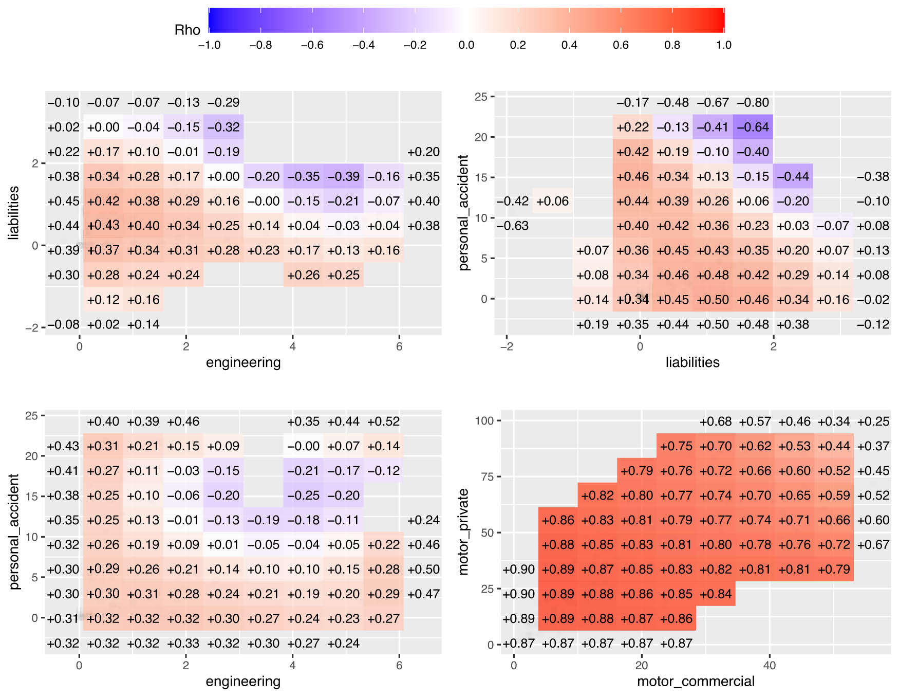
LGC maps claim payouts of different pairs of LoBS for Kenya data.
Our analysis is divided into three parts. First, we used the LGC to model dependency structures of seven LoBs using 174 monthly average claim payouts in millions of Kenyan shillings. These lines of business include motor private (MP), motor commercial (MC), workers’ compensation (WC), fire industrial (FI), liabilities (LI), engineering (EN), and personal accidents (PA). We calculate the local correlations and perform the independence test using Pearson correlation (linear) and LGC test (both linear and nonlinear)
Second, we utilized LGC and HMMs to analyze the time-varying temporary dependence in 699 weekly average claim payouts for auto insurance (motor commercial and motor private LoBs) and 315 claim payouts for homeowner’s insurance (house and content LoBs) from Kenya and Norway, respectively. Both datasets were adjusted for inflation.
Finally, we used the auto insurance LoB data to demonstrate a risk management application by simulating from the fitted LGC model and calculating VaRs. We fit copulas to the data and compute the VaRs using the Monte Carlo simulation approach and compare the VaR results of the LGC model with those of the corresponding copulas.
3 Results
The findings provide an analysis of local correlations among different LoBs and regimes in general insurance. In Section 3.1, we present local Gaussian correlation LGC maps and a table summarizing tests for both linear and nonlinear dependence based on aggregated monthly claims payouts using the Kenyan data. The LGC maps illustrate varying correlation structures across different regions, while the table details statistical test results assessing the dependence. Section 3.2 includes Gaussian HMM plots and LGC plots for original and regime-specific data based on weekly claims payout from Kenya on motor insurance LoBs and Norway on home owners insurance LoBs, The results of the bootstrap test to measure asymmetric dependence structure are presented in Table A3 in appendix A.3, and finally, Section 3.3 covers risk modeling using value-at-risk where we present a risk management application. We also present results on structural breaks analysis in Appendix B and additional results on parameter estimates A.1, model comparisons A.2, A.3, diagnostic checks A.4, and short-term forecasts A.4.1
3.1 Dependence modeling using LGC for general Insurance LoBs
Figure 1 shows LGC maps revealing nonlinear relationships between LoB pairs: liabilities vs engineering (
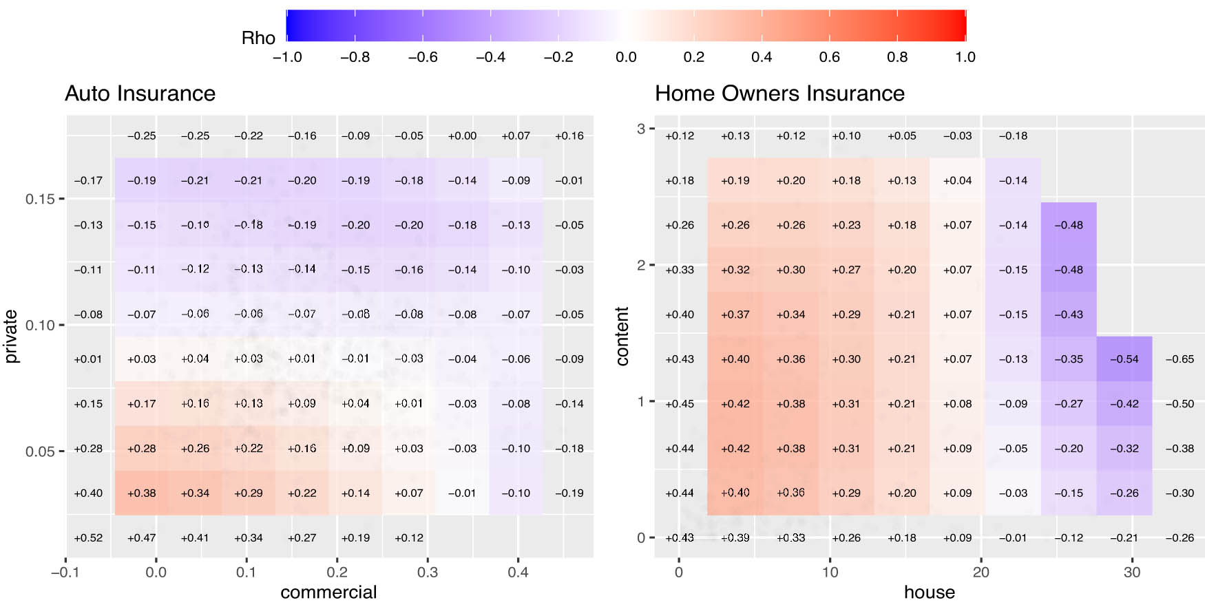
LGC maps of average weekly claim payouts of auto and homeowners insurance of LoBS.
Pair-wise correlation with p-values of ordinary correlation test and LGC test for independence
| Variables pairs | Pearson’s
|
|
|
|---|---|---|---|
| Engineering vs fire-industrial | 0.43 | 0.00*** | 0.00*** |
| Engineering vs liabilities | 0.14 | 0.16 | 0.00*** |
| Engineering vs motor-commercial | 0.34 | 0.00*** | 0.00*** |
| Engineering vs motor-private | 0.42 | 0.00*** | 0.00*** |
| Engineering vs workers-compensation | 0.40 | 0.00*** | 0.00*** |
| Engineering vs personal accident | 0.20 | 0.05* | 0.02** |
| Fire-industrial vs liabilities | 0.43 | 0.00*** | 0.00*** |
| Fire-industrial vs motor-commercial | 0.51 | 0.00*** | 0.00*** |
| Fire-industrial vs motor-private | 0.56 | 0.00*** | 0.00*** |
| Fire-industrial vs workers-compensation | 0.40 | 0.00*** | 0.00*** |
| Fire-industrial vs personal-accidents | 0.25 | 0.01** | 0.00*** |
| Liabilities vs motor-commercial | 0.27 | 0.01** | 0.00*** |
| Liabilities vs motor-private | 0.44 | 0.00*** | 0.00*** |
| Liabilities vs worker-compensation | 0.37 | 0.00*** | 0.00*** |
| Liabilities vs personal-accidents | 0.17 | 0.08* | 0.00*** |
| Motor-commercial vs motor-private | 0.78 | 0.00*** | 0.00*** |
| Motor-commercial vs workers-compensation | 0.66 | 0.00*** | 0.00*** |
| Motor-commercial vs personal-accidents | 0.47 | 0.00*** | 0.00*** |
| Motor-private vs workers-compensation | 0.70 | 0.00*** | 0.00*** |
| Motor-private vs personal-accidents | 0.49 | 0.00*** | 0.00*** |
| Workers-compensation vs personal-accidents | 0.36 | 0.00*** | 0.00*** |
Significance level: ***(1%), **(5%), *(10%).
The standard Pearson correlation test assessed linear dependencies, while the LGC test examined both linear and nonlinear dependencies based on the statistics in Section 2.2 and equation (4). All four graphs in Figure 1 indicate a positive correlation in the lower left tail (low payouts) and a weak or negative correlation in the upper right tail (high payouts). A moderate to weak correlation appears in the center. The nonparametric LGC independence test results in Table 3 reveal these nonlinear relationships, highlighting local correlations that traditional methods might overlook. Table 3 presents Pearson’s
3.2 Dependence modeling using LGC-HMM framework for weekly claims of Motor and Home insurance LoBs
Figure 2 presents the LGC maps of weekly claim payouts for auto and homeowners insurance from Kenya and Norway before applying regime-switching models. The plots reveal nonlinear and heterogeneous dependencies across different claim amount ranges. For auto insurance, local correlations range from moderately negative (
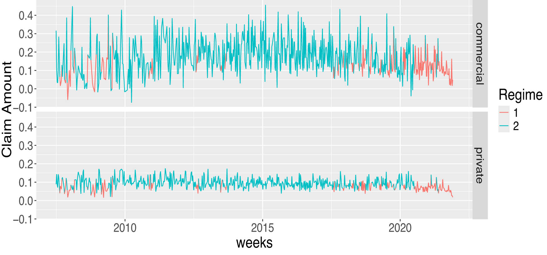
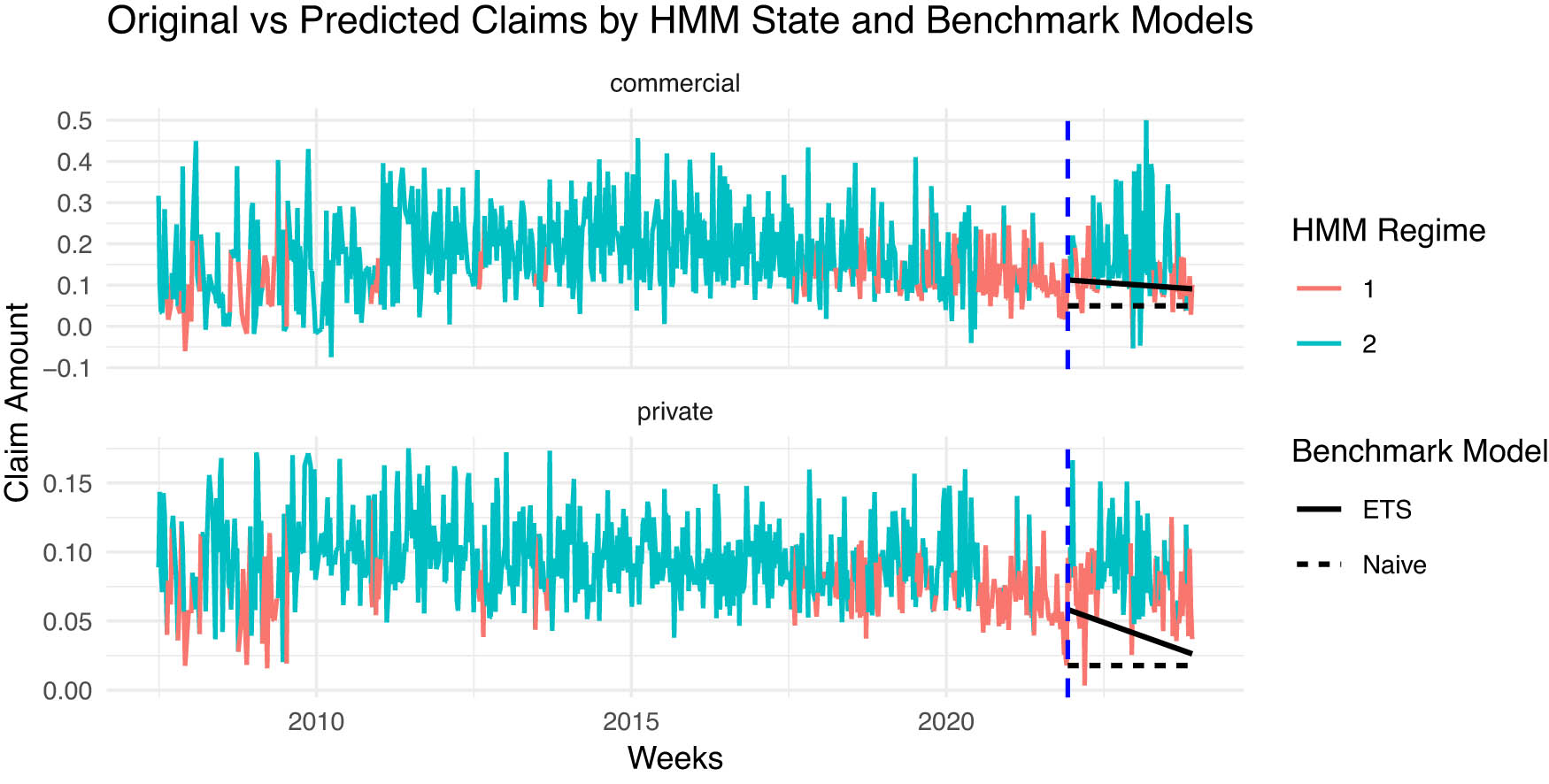
Two-regime time-varying HMM plot for automobile insurance LoBs.
Regime-specific correlation and LGC independence test results
| Regime | Automobile | Home insurance | ||
|---|---|---|---|---|
| Pearson
|
LGC
|
Pearson
|
LGC
|
|
| 1 | 0.168* | 0.04 | 0.262** | 0.00 |
| 2 |
|
0.00 |
|
0.00 |
| All |
|
0.00 | 0.163 | 0.00 |
Significance level: ***(1%), **(5%), *(10%).
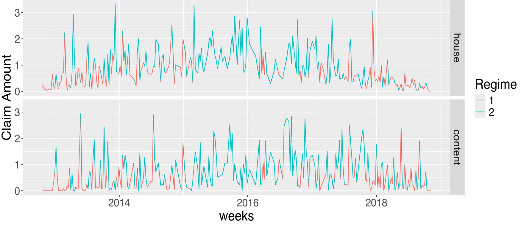
Two-regime time-varying HMM plot of house and content insurance.
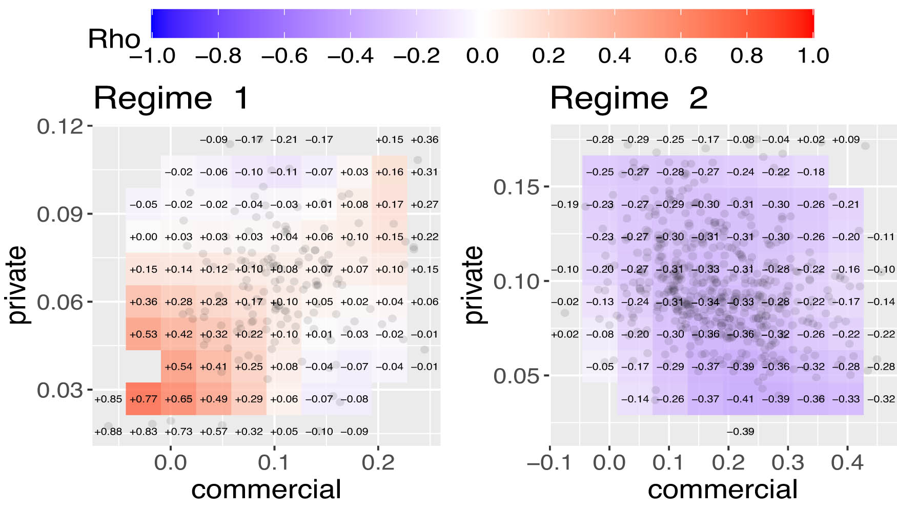
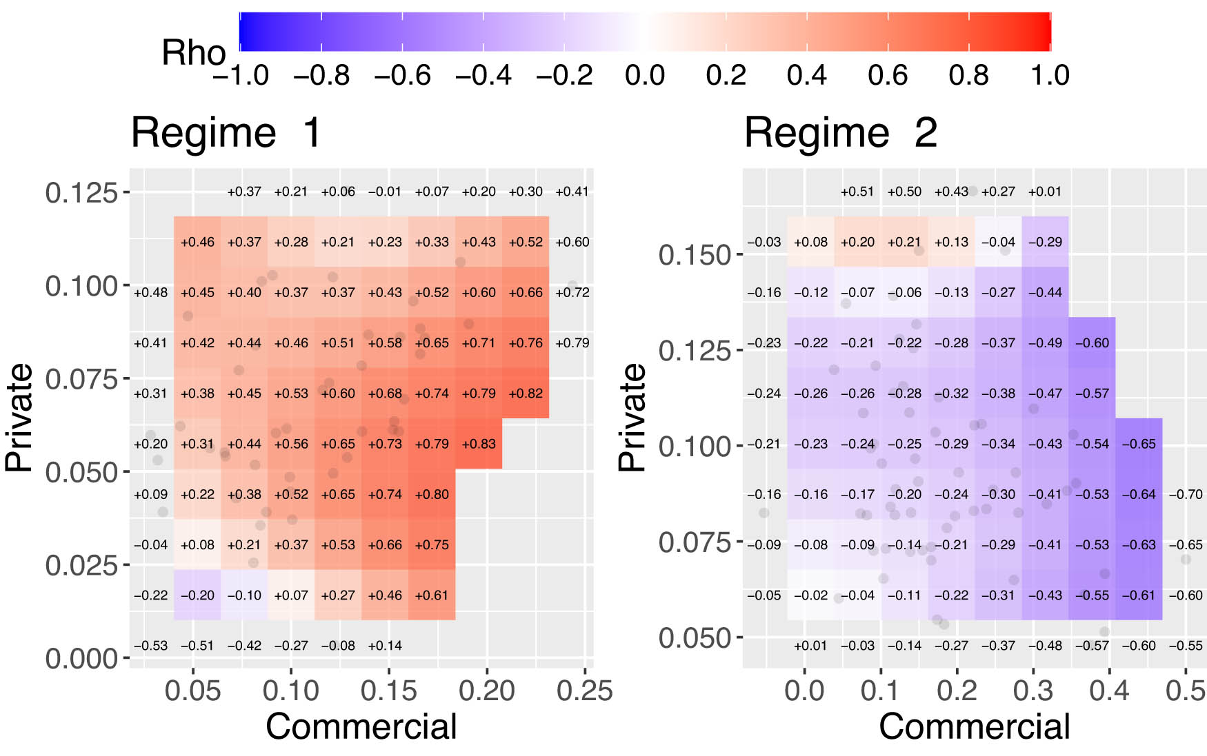
LGC plots of showing nature of time-varying dependence for each of the two regimes for Auto Insurance.
The Gaussian-HMM classified both datasets into two regimes as presented in Figures 3 and 4. In a supplementary material, we present results for the three-regime Gaussian HMM and the t-distribution HMM. By comparing the HMM classifications in Figure 3 with historical events in Kenya, it is found that the HMM can effectively identify crisis periods. Regime 1 is associated with the 2007–2008 Kenyan political crisis [12], the COVID-19 outbreak in 2021, and short periods in regime 1, which could be weeks with terrorist attacks [34] or strikes. Regime 2 appears to represent periods of economic stability or noncrisis periods and claim payout are higher in that period. For home insurance data in Figure 4, regime 1 indicates lower payouts compared to regime 2, without clear patterns except in the period around the end of 2015 to early 2016 where all observations were in regime 2. This outcome could be related to the fall of the oil price in 2015 that impacted Norway’s economy [25].
In Table 4, we compare regimes 1 and 2 by their average weekly claims payouts. Both show nonnormality, indicated by high skewness and kurtosis coefficients. Regime 2 has notably higher volatility, with larger variances and kurtosis for both LoBs. This is emphasized by higher standard errors in regime 2 compared to regime 1 in both LoBs and datasets.
Descriptive statistics for weekly claim payout from automobile and Homeowners insurance LoBs with corresponding regime-specific statistics
| LoB | Regimes |
|
Mean | SD | Median | Min | Max | Skew | Kur | SE |
|---|---|---|---|---|---|---|---|---|---|---|
| Commercial | Regime 1 | 154 | 0.11 | 0.05 | 0.10 |
|
0.24 | 0.17 | 0.26 | 0.00 |
| Regime 2 | 555 | 0.18 | 0.10 | 0.18 |
|
0.46 | 0.26 |
|
0.00 | |
| Original data | 699 | 0.17 | 0.09 | 0.15 |
|
0.46 | 0.53 | 0.48 |
|
|
| Private | Regime 1 | 154 | 0.07 | 0.02 | 0.07 | 0.02 | 0.12 |
|
0.20 | 0.00 |
| Regime 2 | 555 | 0.10 | 0.03 | 0.09 | 0.02 | 0.18 | 0.47 |
|
0.00 | |
| Original data | 699 | 0.09 | 0.03 | 0.09 | 0.02 | 0.18 | 0.44 | 0.09 | 0.00 | |
| House | Regime 1 | 114 | 0.42 | 0.29 | 0.37 | 0.01 | 1.09 | 0.38 |
|
0.03 |
| Regime 2 | 200 | 1.23 | 0.73 | 1.15 | 0.10 | 3.31 | 0.72 | 0.03 | 0.06 | |
| Original data | 314 | 0.88 | 0.70 | 0.69 | 0.01 | 3.31 | 1.17 | 1.05 | 0.04 | |
| Content | Regime 1 | 114 | 0.18 | 0.17 | 0.13 | 0.00 | 0.58 | 0.77 |
|
0.02 |
| Regime 2 | 200 | 1.03 | 0.74 | 0.98 | 0.00 | 2.95 | 0.65 |
|
0.06 | |
| Original data | 314 | 0.66 | 0.71 | 0.41 | 0.00 | 2.95 | 1.29 | 0.96 | 0.04 |
In Table 5, the null hypothesis of independence was rejected in both regimes, with p-values
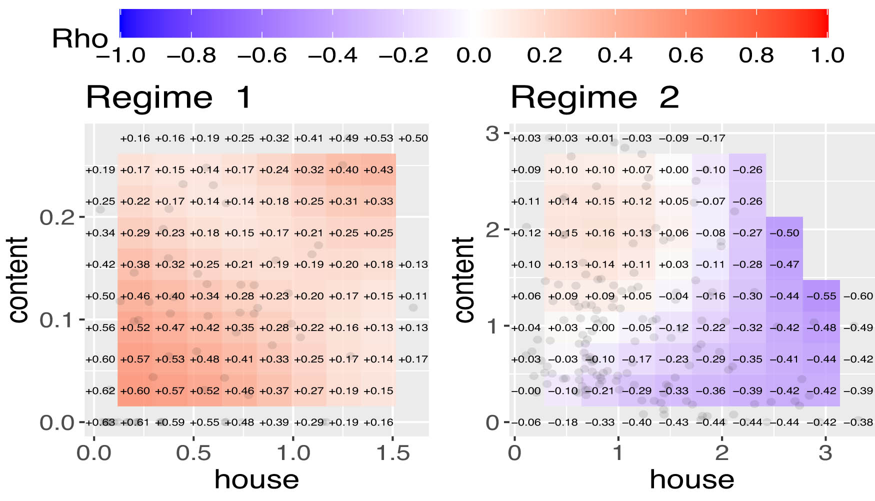
LGC plots showing nature of time varying dependence for each of the two regimes in Home owners Insurance.
The results for testing whether the dependence structure between the claim payouts varies across the regimes using the test statistic described in Section 2.4 and detailed in equation (5) gives a
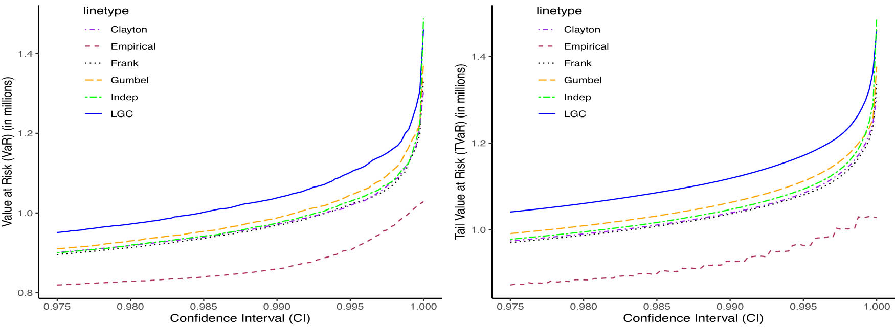
VaR and TVaR at different confidence intervals for No Regime data.
The plots in Figure 5 show regime-specific LGC maps for auto data from Kenya. The results reveal that in regime 1, the local correlations are predominantly positive, particularly in the lower left tail, while they tend to be close to zero or negative in the lower right tail and upper left corner. This pattern indicates the existence of nonlinear tail dependence. In addition, Table 5 shows that in regime 2, the correlation is negative, with a Pearson correlation coefficient of
Furthermore, in regime 1, the LGC test for independence yields a
The aforementioned analysis indicates that using HMMs and LGC to examine dependencies reveals a significant difference in the dependence patterns between the two regimes. These methodologies have enhanced our understanding of complex structures and temporal dynamics, helped us identify local correlations and transitions over time, and improved our comprehension of risk relationships.
3.3 Risk modeling using value-at-risk and tail value at risk
To quantify potential extreme losses in insurance claims, we employ two widely used risk measures. The VaR at confidence level
The Tail Value-at-Risk (also called Expected Shortfall) at level
We analyzed weekly data from Kenya, combining claims from two business lines (motor private and motor commercial) into a single portfolio with equal weights. We modeled the joint distribution of claims using copulas and LGC densities, generating 50,000 simulated observations per model. These simulations were transformed using the inverse lognormal distribution with a log-mean of 0.5 and a log-standard deviation of 0.2. Based on the transformed data, we estimated VaR and TVaR at various confidence levels. Historical estimates of VaR and TVaR, for a model called “Empirical,” were included as benchmarks alongside the copula-based and LGC-based risk measures.
Table 6 reports 99% VaR and TVaR estimates in millions of Kenyan Shillings for several models under three scenarios: No Regime (full sample), Regime 1, and Regime 2. The regime structure is inferred from the fitted HMM in (Figure 3) and supported by LGC dependence maps (Figure 5). The LGC model delivers the highest VaR and TVaR estimates across the No regime and Regime 1 cases, confirming its sensitivity to changes in dependence structure and its ability to capture heightened tail risk, especially in Regime 1. In contrast, the historical VaRs, i.e., the “Empirical” model provide the lowest estimates, reflecting limited capacity to account for evolving dependence dynamics. The Independence model shows minimal variation across regimes, underscoring its inability to detect shifts in tail dependence. The Clayton and Gumbel copulas are excluded from Regime 2 due to their restriction to positive dependence, making them unsuitable for regimes with negative or weakening dependencies. The Frank copula performs moderately well, with lower estimates in Regime 2 reflecting a shift to less severe joint tail events. Figures 7, 8, and 9 visually demonstrate the LGC model’s ability to adapt to structural changes in dependence, with its curves consistently lying above other models in the tail regions, especially under regime-specific scenarios. The results in Figures 7–9 visually illustrate how risk estimates, both VaR and TVaR, increase with higher confidence intervals across all scenarios, as expected. In the No Regime and Regime 1 cases, the Independence copula yields consistently lower risk estimates due to its zero-dependence assumption, which fails to capture actual tail dependence and may thus underestimate extreme losses.
99% VaR and TVaR for different copulas in millions of Kenyan Shillings under No Regime and Regime scenarios
| No Regime | Regime 1 | Regime 2 | ||||
|---|---|---|---|---|---|---|
| Model | VaR | TVaR | VaR | TVaR | VaR | TVaR |
| Independence | 0.968880 | 1.034113 | 0.968880 | 1.034113 | 0.977789 | 1.047075 |
| LGC | 1.037779 | 1.118604 | 1.059460 | 1.144846 | 0.943067 | 1.012367 |
| Frank | 0.975142 | 1.042112 | 0.995103 | 1.065286 | 0.915325 | 0.986832 |
| Clayton | 0.972135 | 1.038845 | 0.991025 | 1.061449 | — | — |
| Gumbel | 0.987532 | 1.062863 | 1.026035 | 1.125845 | — | — |
| Empirical | 0.859667 | 0.927649 | 0.896448 | 0.931381 | 0.834478 | 0.863790 |
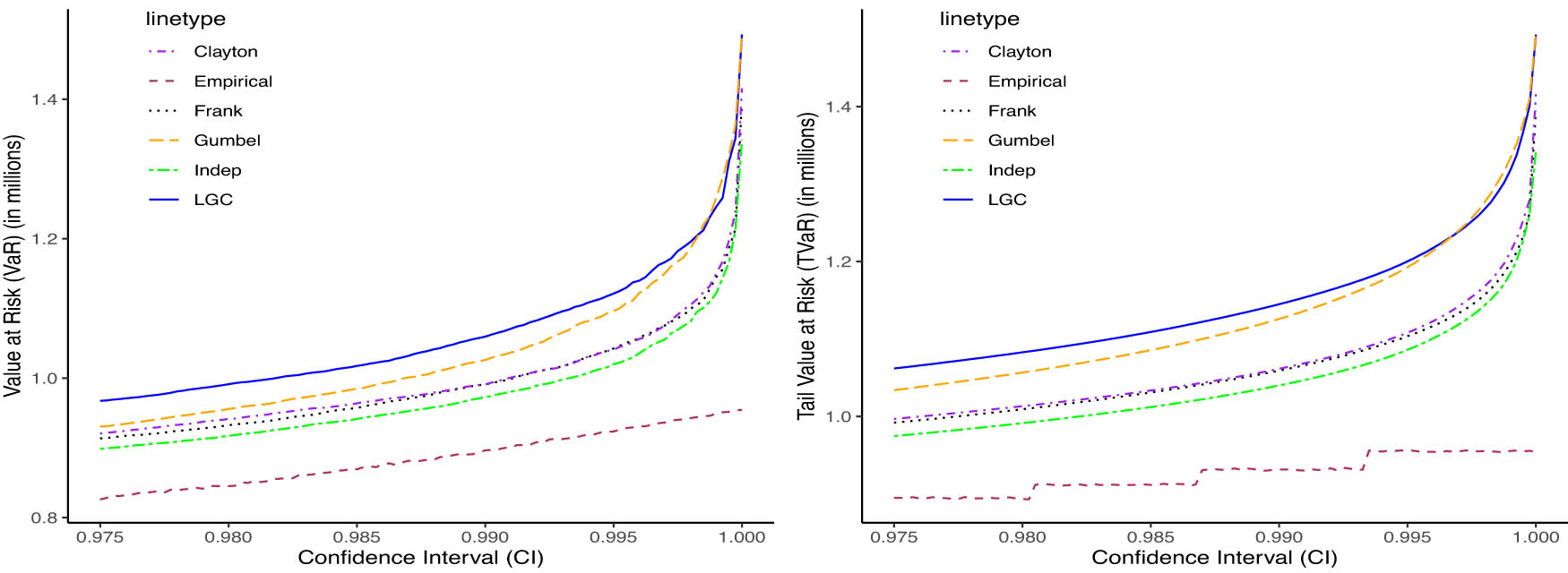
VaR and TVaR at different confidence intervals for Regime 1 data.
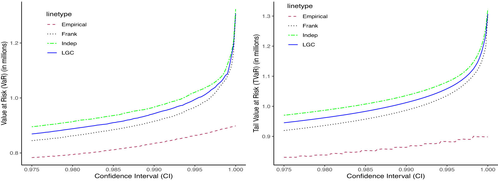
VaR and TVaR at different confidence intervals for Regime 2 data.
The empirical (historical) model also produces low estimates across all scenarios, as it does not incorporate structural dynamics or tail dependencies, limiting its responsiveness to shifts in joint behavior. In contrast, the LGC model demonstrates clear sensitivity to changing dependence structures, adapting its estimates to underlying regime characteristics and consistently producing higher, more cautious values. In Regime 2, where negative dependence dominates, the Independence model overestimates risk by ignoring diversification effects. The Frank copula adjusts more effectively, capturing the benefits of negative correlation and yielding significantly lower VaR and TVaR estimates. Notably, the LGC model remains robust across all regimes, flexibly responding to positive and negative dependence structures.
4 Discussion and conclusion
This study introduces a novel framework that integrates LGC with HMMs to model regime-dependent dependencies in insurance data. The combination of LGC and HMM allows for flexible modeling of nonlinear, asymmetric dependencies that evolve over time. Unlike standard copula models or constant-correlation frameworks, the LGC-HMM captures localized dependence structures and transitions between latent states. This addresses a known limitation in traditional HMMs, which often assume homogeneous dependence within each regime.
Our results reveal that dependence structures between claim lines vary significantly across regimes. These findings are consistent with Gundersen et al. [22], who emphasize the importance of modeling regime-specific and asymmetric dependence. In particular, we observe that dependencies intensify during high-risk regimes – an effect often overlooked by traditional models. This regime-specific view of dependence is especially relevant for dynamic risk assessment and stress testing in nonlife insurance.
From a practical standpoint, the LGC-HMM framework supports risk-sensitive decision-making. By identifying periods in which dependencies between lines of business strengthen, the model facilitates more accurate assessments of joint tail risk. This capability is especially valuable for dynamic solvency capital allocation under regulatory frameworks such as solvency II. It enables insurers to recognize when diversification benefits deteriorate, prompting timely adjustments to capital buffers or reinsurance strategies. Furthermore, incorporating regime-switching behavior captures cyclical or structural market shifts, enhancing the model’s utility for pricing, reserving, and portfolio management.
Our work builds upon prior applications of HMMs in insurance, including Norberg [36], Bulla and Bulla [11], and Mamon and Elliott [32], which focused on capturing unobserved risk factors and structural changes. However, these studies typically relied on linear or Gaussian dependence assumptions within regimes. By integrating LGC, we contribute to the semiparametric dependence modeling literature [38,44] and extend recent work by Gundersen et al. [22] to nonlife insurance applications.
While LGC does not require global Gaussian dependence, our current framework assumes Gaussian emissions within each regime. This may reduce robustness in the presence of heavy-tailed claims a common feature in insurance. As noted by Gundersen et al. [22], failing to account for leptokurtosis can lead to underestimated risks. Future extensions could consider Student-
Nevertheless, the robustness of the proposed framework to leptokurtosis is supported by the findings of Gundersen et al. [22], who show that replacing Gaussian regime-wise distributions with heavy-tailed alternatives such as the Student-
In addition, the assumption of geometrically distributed regime durations in standard HMMs may not adequately reflect real-world insurance cycles. Incorporating hidden semi-markov models, as demonstrated by Shi et al. [42] in weather-related claims, allows for more flexible state duration modeling. Covariate-driven or time-varying transition probabilities may also increase the model’s adaptability.
While our model primarily addresses joint tail risk through the use of VaR and TVaR, a promising direction for future research is the integration of conditional value-at-risk (CoVaR) to assess systemic risk spillovers across lines of business. As introduced by Tobias and Brunnermeier [46], CoVaR measures the risk of one component conditional on another being in distress, making it particularly suitable for analyzing interdependencies and systemic vulnerabilities. However, implementing CoVaR within our current LGC-HMM framework poses significant computational challenges, given the presence of regime-switching behavior and the complexity of time-varying dependence structures [8]. As such, we defer this extension to future work. Nevertheless, our results already demonstrate that the LGC model effectively captures nonlinear dependence and regime-specific tail dynamics, providing a robust foundation for advancing systemic risk modeling.
In conclusion, the LGC-HMM framework significantly advances modeling dynamic, regime-dependent structures in insurance data. By capturing localized, nonlinear dependencies and adapting to structural shifts, it yields more accurate and responsive VaR and TVaR estimates, particularly under high-risk regimes. Integrating LGC with regime-switching dynamics gives actuaries a powerful and interpretable tool for modern risk assessment and crisis-sensitive pricing. While the model demonstrates strong empirical performance, certain data limitations, such as potential reporting lags and aggregation effects, may affect the accuracy of regime identification and predictive precision. Addressing these challenges presents an avenue for future refinement and validation across broader datasets and insurance contexts.
Acknowledgments
We extend our gratitude to our sponsors, the MATH4SDG project’s principal investigators, and the participants and organizers of the 2023 Actuarial Finance and Risk Conference (AFRIC). Z. Afazali sincerely thank EMS-Simons for Africa for the additional financial support for this research, which included funds for extended research visits and child support. We are also grateful to the anonymous reviewers and the editorial team for their constructive feedback and valuable suggestions, which significantly improved the quality of this work.
-
Funding information: This work has been supported by the Mathematics for Sustainable Development (MATH4SDG) project, which is a research and development project running in the period 2021–2026 at Makerere University-Uganda, the University of Dar es Salaam-Tanzania, and the University of Bergen-Norway, funded through the NORHED II program under the Norwegian Agency for Development Cooperation (NORAD, project no 68105).
-
Author contributions: Zabibu conceptualized the study, conducted the primary analysis, and drafted the manuscript under the supervision of Bård, Juma, and Saint, who provided critical feedback. Kristian collaborated with Zabibu to review and update the computational codes. All authors reviewed the results, approved the final manuscript, and consented to its submission.
-
Conflict of interest: The authors declare no conflicts of interest.
-
Data availability statement: The datasets presented in this article are publicly available at https://doi.org/10.6084/m9.figshare.25904902. The the supplementary material comprises extra LGC maps, a three-regime HMM extension, results of model comparisons, and R code for the implementation of the models.
Appendix A Additional results
In this appendix, we present additional results on parameter estimates for the HMMs and copula models, model comparisons between HMMs with different number of regimes, diagnostic checks, and short-term forecast from the fitted models.
A.1 HMM parameters for two regime HMM
The Table A1 presents the HMM parameter estimates for auto and homeowners insurance on the original scale. In both datasets, State 1 represents a high-claim regime with larger means than State 2. Homeowners’ insurance shows significantly higher mean values and greater variability, as indicated by larger variances and covariances, suggesting more volatile claim behavior. Transition probabilities reveal that auto insurance is more likely to switch from high- to low-claim states, while homeowners insurance shows a more balanced and persistent risk pattern. These differences highlight the need for tailored risk management approaches across the two insurance lines.
Estimated HMM parameters
| Parameter | Auto insurance | Homeowners insurance | ||
|---|---|---|---|---|
| Estimate | Std. error | Estimate | Std. error | |
|
Mean vector
|
||||
|
|
0.1115 | 0.0081 | 3.6835 | 0.4116 |
|
|
0.1838 | 0.0068 | 11.0889 | 0.5603 |
|
|
0.0690 | 0.0036 | 0.1018 | 0.0172 |
|
|
0.0978 | 0.0019 | 0.9183 | 0.0585 |
|
Covariance elements
|
||||
|
|
0.0601 | 0.0951 | 2.7764 | 0.1179 |
|
|
0.0002 | 0.0021 | 1.0210 | 0.0145 |
|
|
0.0204 | 0.1105 | 0.0958 | 0.1598 |
|
|
0.0975 | 0.0340 | 7.1368 | 0.0537 |
|
|
|
0.0020 | 0.9011 | 0.0566 |
|
|
0.0272 | 0.0359 | 0.7123 | 0.0530 |
|
Transition probabilities
|
||||
|
|
0.2364 | 0.5924 | 0.2298 | 0.2171 |
|
|
0.7636 | 0.4754 | 0.4969 | 0.2462 |
A.2 Copula parameters and goodness-of-fit test
We fit copulas to the original data and regime-specific data; then computed VaRs presented in Section 3.3, and in Table A2. The goodness-of-fit test was conducted using Cramér–von Mises statistic (Sn) within a parametric bootstrap framework [18]. This approach assesses the discrepancy between the empirical copula and the fitted copula model, with p-values indicating the model’s adequacy in capturing the dependence structure.
Comparison of copula parameters, statistics, and
| Data type | Copula type | Parameter | Statistic |
|
|---|---|---|---|---|
| Original | Gumbel | 1.0950 | 0.0388 | 0.0814 |
| Clayton | 0.0953 | 0.0502 | 0.0045 | |
| Frank | 0.0082 | 0.0369 | 0.0265 | |
| Gaussian | 0.0208 | 0.0383 | 0.0245 | |
| Regime 1 | Gumbel | 1.0959 | 0.0206 | 0.5070 |
| Clayton | 0.3014 | 0.0164 | 0.7048 | |
| Frank | 0.7454 | 0.0193 | 0.5579 | |
| Gaussian | 0.1526 | 0.0178 | 0.6429 | |
| Frank |
|
0.0200 | 0.3462 | |
| Regime 2 | Gaussian | 0.0292 |
|
0.1054 |
The goodness-of-fit test results indicate that copula models perform differently across data regimes. For the original data, the Clayton copula shows a poor fit, while the Gumbel, Frank, and Gaussian copulas exhibit weak evidence of poor fit. In Regime 1, all copulas fit the data well, with high p-values indicating no significant issues. However, in Regime 2, both the Gumbel and Clayton copulas show poor fits, while the Frank copula and the Gaussian copula provide reasonable fits. The Frank copula shows near-zero dependence across original data (0.008), weak positive dependence in regime 1 (0.745), and strong negative dependence in regime 2 (
A.3 Comparison of two regime and three regime HMM results
From Table A3, in the case of the three-regime HMM, we observed no difference in dependence between all paired regimes for the automobile data. However, for homeowners’ insurance data, a significant difference in dependence structure was noted between pairs of regimes 1 and 2, and regimes 1 and 3, while no difference in dependence structure was observed between regimes 2 and 3. The HMM time plot and LGC maps for the three-regime HMM model are in supplementary material. Upon comparing the two-regime and three-regime HMM across both datasets using AIC and BIC, for the automobile data, the two-regime model is superior to a three-regime model. Conversely, for homeowners’ insurance LoBs, the results favor a three-regime model over a two-regime model. However, due to model complexity and few observations in one of the regimes, a two-regime model is still preferred.
Results of model comparisons and bootstrap dependence tests for 2- regime and 3 regime HMM for automobile and homeowners insurance LoBs
| Data type | Model type | regimes
|
LLK | AIC | BIC |
|
|---|---|---|---|---|---|---|
| Auto insurance average claim cost per week | 2-regime normal |
|
|
4178.574 | 4187.883 | 0.000 |
| Auto insurance average claim cost per week | 3-regime normal |
|
-2133.32 | 4272.639 | 4286.623 | 0.379 (1 and 2) 0.443 (1 and 3) 0.243 (2 and 3) |
| Homeowner’s insurance claims cost per week | 2-regime normal |
|
|
892.6551 | 883.3991 | 0.000 |
| Homeowner’s insurance claims cost | 3-regime normal |
|
|
788.811 | 774.927 | 0.000 (1 and 2) 0.000 (1 and 3) 0.313 (2 and 3) |
A.4 Diagnostic checks using auto correlation functions (ACF)
Let
In the Figure A1(a) and (b), the original series for all LoBs exhibit significant autocorrelation, indicating strong temporal dependence in claim patterns. After HMM model fitting, the residual ACFs show a marked reduction in autocorrelation, particularly for the private auto and home content lines, suggesting adequate model performance.
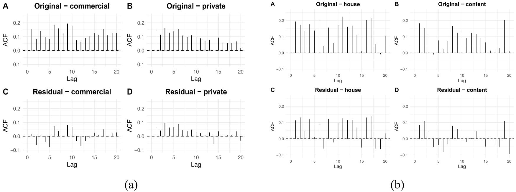
ACFs of original and residuals of HMM model for both auto and home insurance data. (a) Auto insurance LoBs and (b) home insurance LoBs.
A.4.1 Forecast dynamics and regime-specific dependencies in auto insurance claims
As figure A2 shows that Regime 1 and Regime 2 exhibit distinct dynamics in commercial and private claim amounts, with the dashed vertical line marking the forecast period’s start. Benchmark forecasts include the Naive model, which uses the last observed value, and exponential smoothing (ETS) with exponentially weighted averages. HMM forecasts reveal regime-dependent variations missing in these benchmarks. Figure A3 displays LGC maps from HMM forecasts, highlighting strong positive local dependence in Regime 1 and weaker or negative dependence in Regime 2, especially at higher commercial claim levels. These results indicate structural shifts in predicted claims across regimes.
Actual and forecasted weekly auto insurance claims by HMM regime and benchmark models.
LGC maps for HMM-based predicted claims showing regime-specific local dependence between commercial and private claims under regime 1 (left) and regime 2 (right).
B Rolling mean, rolling standard deviation, and change point detection
To analyze structural changes and volatility in weekly insurance claims, we apply rolling statistics and change point detection. Rolling mean and standard deviation, computed over a fixed window
Structural breaks are identified using the PELT algorithm, which minimizes a penalized cost function:
where
B.1 Empirical evidence of regime changes in claim behavior
The Figures A4(a), (c), and (e) show variations in house and content insurance claims over time. The rolling mean and standard deviation plots highlight fluctuations in claim amounts from 2012 to 2018. House claims are more volatile with frequent spikes, while content claims show moderate variability. Change point detection plots reveal structural breaks in mean levels for both LoBs, indicating shifts in claim behavior. The Figures A4(b), (d), and (f) show significant variations in commercial and private insurance claims over time. Since 2015, commercial claims exhibit an upward trend and increased volatility, reflecting greater sensitivity to external changes. In contrast, private claims are stable but show fluctuations in mean and variability, indicating cyclical behavior. Change point detection plots demonstrate distinct mean-level shifts for both claim types, suggesting varying claim dynamics. These findings highlight dynamic risk patterns and support models that capture time-varying structures in insurance data.
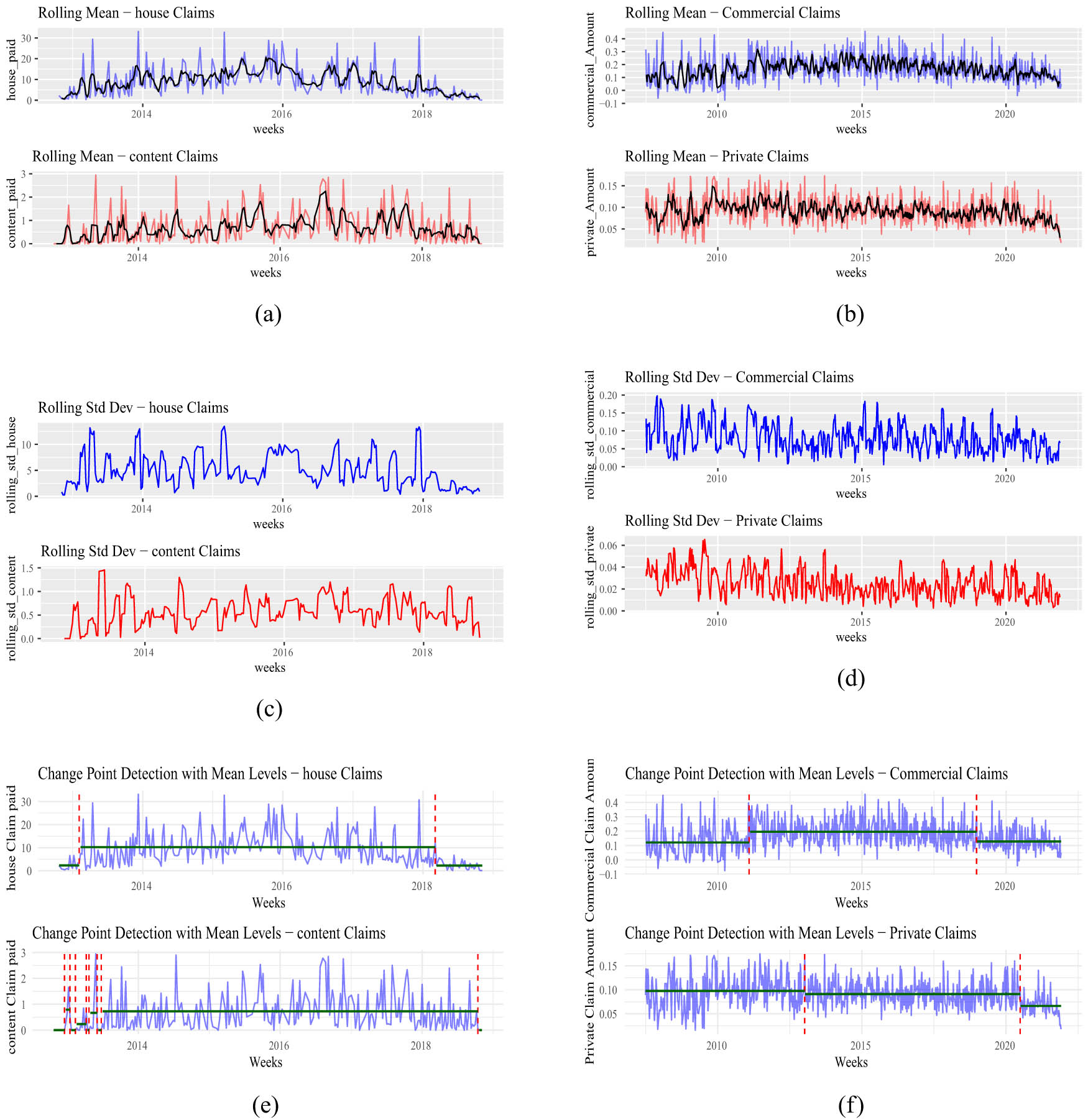
Rolling mean, rolling standard deviation, and change points plots for auto and home insurance claims (commercial, private, house, and content) from 2008 to 2021. (a) rolling mean (house an content), (b) rolling mean (commercial and private), (c) rolling std dev (house an content), (d) rolling std dev (commercial and private), (e) change points (house and content), and (f) change points (commercial and private).
C Estimating the LGC parameters
The minimization of
where
We define the population value
In [45], the authors demonstrated that if a unique population vector
Both the population vectors
As
If we assume that
by the ergodic theorem in the time series case or by the law of large numbers.
Let
Therefore, ignoring solutions that yield
D Estimation of the likelihood using forward and backward algorithms
The forward algorithm enables a recursive computation of the likelihood. Define
where the recursion is given by
After processing all observations, the likelihood is obtained as follows:
Similarly, the backward algorithm computes
with recursion
for
The forward and backward probabilities are defined for
The smoothing probabilities, corresponding to the conditional probability of being in regime
In this article, we employ local decoding, where the most probable regime at each time
Thus, the most probable regime at time
E Bootstrap test procedure
We rely on bootstrap testing for its robustness in handling small sample sizes and uncertain data distributions. By sidestepping strict assumptions and leveraging resampling techniques, the bootstrap testing enhances the reliability of our analysis, allowing for a more nuanced understanding of inter-line dependencies within insurance claim payouts. The bootstrap procedure employed here works as follows: From the set of observations
where
References
[1] Alexeev, V., Ignatieva, K., & Liyanage, T. (2019). Dependence modelling in insurance via copulas with skewed generalised hyperbolic marginals. Studies in Nonlinear Dynamics & Econometrics, 25(2), 20180094. 10.1515/snde-2018-0094Search in Google Scholar
[2] Araichi, S., de Peretti, C., & Belkacem, L. (2017). Reserve modelling and the aggregation of risks using time varying copula models. Economic Modelling, 67, 149–158. 10.1016/j.econmod.2016.11.016Search in Google Scholar
[3] Avanzi, B., Taylor, G., & Wong, B. (2016). Correlations between insurance lines of business: An illusion or a real phenomenon? some methodological considerations. ASTIN Bulletin: The Journal of the IAA, 46(2), 225–263. 10.1017/asb.2015.31Search in Google Scholar
[4] Bacri, T., Berentsen, G. D., Bulla, J., & Hølleland, S. (2022). A gentle tutorial on accelerated parameter and confidence interval estimation for hidden Markov models using template model builder. Biometrical Journal, 64(7), 1260–1288. 10.1002/bimj.202100256Search in Google Scholar PubMed PubMed Central
[5] Berentsen, G. D., Kleppe, T. S., & Tjøstheim, D. B. (2014). Introducing local gauss, an r package for estimating and visualizing local Gaussian correlation. Journal of Statistical Software, 56, 1–18. 10.18637/jss.v056.i12Search in Google Scholar
[6] Berentsen, G. D., Støve, B., Tjøstheim, D., & Nordbø, T. (2014). Recognizing and visualizing copulas: an approach using local Gaussian approximation. Insurance: Mathematics and Economics, 57, 90–103. 10.1016/j.insmatheco.2014.04.005Search in Google Scholar
[7] Bernardi, M., Catania, L., & Petrella, L. (2014). t-student copula mixtures and tail dependence: An application to systemic risk. Journal of Econometrics, 182(2), 364–378. Search in Google Scholar
[8] Bernardi, M., Maruotti, A., & Petrella, L. (2017). Multiple risk measures for multivariate dynamic heavy-tailed models. Journal of Empirical Finance, 43, 1–32. 10.1016/j.jempfin.2017.04.005Search in Google Scholar
[9] Bolancé, C., Bahraoui, Z., & Artís, M. (2014). Quantifying the risk using copulae with nonparametric marginals. Insurance: Mathematics and Economics, 58, 46–56. 10.1016/j.insmatheco.2014.06.008Search in Google Scholar
[10] Bolance, C., Guillen, M., Pelican, E., & Vernic, R. (2008). Skewed bivariate models and nonparametric estimation for the cte risk measure. Insurance: Mathematics and Economics, 43(3), 386–393. 10.1016/j.insmatheco.2008.07.005Search in Google Scholar
[11] Bulla, J., & Bulla, I. (2006). Stylized facts of financial time series and hidden semi-markov models. Computational Statistics & Data Analysis, 51(4), 2192–2209. 10.1016/j.csda.2006.07.021Search in Google Scholar
[12] Cheeseman, N. (2008). The kenyan elections of 2007: An introduction. Journal of Eastern African Studies, 2(2), 166–184. 10.1080/17531050802058286Search in Google Scholar
[13] Chua, C. L., & Tsiaplias, S. (2018). A Bayesian approach to modeling time-varying cointegration and cointegrating rank. Journal of Business & Economic Statistics, 36(2), 267–277. 10.1080/07350015.2016.1166117Search in Google Scholar
[14] Cossette, H., Gaillardetz, P., Marceau, EE, & Rioux, J. (2002). On two dependent individual risk models. Insurance: Mathematics and Economics, 30(2), 153–166. 10.1016/S0167-6687(02)00094-XSearch in Google Scholar
[15] Diers, D., Eling, M., & Marek, S. D. (2012). Dependence modeling in non-life insurance using the Bernstein copula. Insurance: Mathematics and Economics, 50(3), 430–436. 10.1016/j.insmatheco.2012.02.007Search in Google Scholar
[16] Embrechts, P., McNeil, A., & Straumann, D. (2002). Correlation and dependence in risk management: properties and pitfalls. Risk Management: Value at Risk and Beyond, 1, 176–223. 10.1017/CBO9780511615337.008Search in Google Scholar
[17] Forney, G. D. (1973). The viterbi algorithm. Proceedings of the IEEE, 61(3), 268–278. 10.1109/PROC.1973.9030Search in Google Scholar
[18] Genest, C., & Favre, A.-C. (2007). Everything you always wanted to know about copula modeling but were afraid to ask. Journal of hydrologic engineering, 12(4), 347–368. 10.1061/(ASCE)1084-0699(2007)12:4(347)Search in Google Scholar
[19] Genest, C., & Scherer, M. (2020). Insurance applications of dependence modeling. Dependence Modeling, 8(1), 93–106. 10.1515/demo-2020-0005Search in Google Scholar
[20] Ghosh, I., Watts, D., & Chakraborty, S. (2022). Modeling bivariate dependency in insurance data via copula: A brief study. Journal of Risk and Financial Management, 15(8), 329. 10.3390/jrfm15080329Search in Google Scholar
[21] Grimmett, G., & Stirzaker, D. (2020). Probability and random processes. Oxford, United Kingdom: Oxford University Press. Search in Google Scholar
[22] Gundersen, K., Bacri, T., Bulla, J., Hølleland, S., Maruotti, A., & Støve, B. (2024). Testing for time-varying nonlinear dependence structures: Regime-switching and local Gaussian correlation. Scandinavian Journal of Statistics, 51(3), 1012–1060. 10.1111/sjos.12744Search in Google Scholar
[23] Hamilton, J. D. (1989). A new approach to the economic analysis of nonstationary time series and the business cycle. Econometrica: Journal of the Econometric Society, 57(2), 357–384. 10.2307/1912559Search in Google Scholar
[24] Huang, X., & Tang, H. (2022). Measuring multi-volatility states of financial markets based on multifractal clustering model. Journal of Forecasting, 41(3), 422–434. 10.1002/for.2820Search in Google Scholar
[25] International Monetary Fund. (2016). Norway: 2016 Article IV Consultation Press Release; Staff Report; and Statement by the Executive Director for Norway. Technical Report 16/214, Washington, D.C: International Monetary Fund. 10.5089/9781498345026.002Search in Google Scholar
[26] Joe, H. (1997). Multivariate models and multivariate dependence concepts. Monographs on Statistics & Applied Probability. Boca Raton, Florida: C&H/CRC. 10.1201/b13150Search in Google Scholar
[27] Killick, R., & Eckley, I. A. (2014). Changepoint: An r package for changepoint analysis. Journal of Statistical Software, 58(3), 1–19. 10.18637/jss.v058.i03Search in Google Scholar
[28] Killick, R., Fearnhead, P., & Eckley, I. A. (2012). Optimal detection of changepoints with a linear computational cost. Journal of the American Statistical Association, 107(500), 1590–1598. 10.1080/01621459.2012.737745Search in Google Scholar
[29] Lane, M. N. (2000). Pricing risk transfer transactions1. ASTIN Bulletin: The Journal of the IAA, 30(2), 259–293. 10.2143/AST.30.2.504635Search in Google Scholar
[30] Langrock, R., & Zucchini, W. (2011). Hidden markov models with arbitrary state dwell-time distributions. Computational Statistics & Data Analysis, 55(1), 715–724. 10.1016/j.csda.2010.06.015Search in Google Scholar
[31] Mamon, R. S., & Elliott, R. J. (2007). Hidden Markov models in finance (vol. 4). New York, USA: Springer. 10.1007/0-387-71163-5Search in Google Scholar
[32] MFarri, F., & Moutanabbir, K. (2022). Risk aggregation and capital allocation using a new generalized archimedean copula. Insurance: Mathematics and Economics, 102, 75–90. 10.1016/j.insmatheco.2021.11.007Search in Google Scholar
[33] Michelot, T. (2022). hmmtmb: Hidden markov models with flexible covariate effects in r. arXiv: http://arXiv.org/abs/arXiv:2211.14139. Search in Google Scholar
[34] Miller E. (2013). Al-Shabab Attack on Westgate Mall in Kenya. Technical report. National Consortium for the Study of Terrorism and Responses to Terrorism. USA: University of Maryland.Search in Google Scholar
[35] Norberg, R. (1993). Prediction of outstanding liabilities in non-life insurance. Astin Bulletin: The Journal of the IAA, 23(1), 95–115. 10.2143/AST.23.1.2005103Search in Google Scholar
[36] Oflaz, Z. (2016). Bivariate hidden markov model to capture the dependency in claim estimate. (Master’s thesis). Ankara, Turkey: Middle East Technical University. Search in Google Scholar
[37] Otneim, H. (2021). lg: An r package for local Gaussian approximations. R Journal, 13(2), 15. 10.32614/RJ-2021-079Search in Google Scholar
[38] Otneim, H., & Tjøstheim, D. (2017). The locally Gaussian density estimator for multivariate data. Statistics and Computing, 27, 1595–1616. 10.1007/s11222-016-9706-6Search in Google Scholar
[39] Rabiner, L. R. (1989). A tutorial on hidden markov models and selected applications in speech recognition. Proceedings of the IEEE, 77(2), 257–286. 10.1109/5.18626Search in Google Scholar
[40] Sancetta, A., & Satchell, S. (2004). The bernstein copula and its applications to modeling and approximations of multivariate distributions. Econometric theory, 20(3), 535–562. 10.1017/S026646660420305XSearch in Google Scholar
[41] Scherer, M., & Stahl, G. (2021). The standard formula of solvency ii: A critical discussion. European Actuarial Journal, 11, 3–20. 10.1007/s13385-020-00252-zSearch in Google Scholar
[42] Shi, Y., Punzo, A., Otneim, H., & Maruotti, A. (2025). Hidden semi-markov models for rainfall-related insurance claims. Insurance: Mathematics and Economics, 120, 91–106. 10.1016/j.insmatheco.2024.11.008Search in Google Scholar
[43] Silverman, B. W. (1986). Density estimation for statistics and data analysis (Vol. 26). New York, USA: CRC Press. Search in Google Scholar
[44] Støve, B., Tjøstheim, D., & Hufthammer, K. O. (2014). Using local Gaussian correlation in a nonlinear re-examination of financial contagion. Journal of Empirical Finance, 25, 62–82. 10.1016/j.jempfin.2013.11.006Search in Google Scholar
[45] Tjøstheim, D., & Hufthammer, K. O. (2013). Local Gaussian correlation: A new measure of dependence. Journal of Econometrics, 172(1), 33–48. 10.1016/j.jeconom.2012.08.001Search in Google Scholar
[46] Tobias, A., & Brunnermeier, M. K. (2016). Covar. The American Economic Review, 106(7), 1705. 10.1257/aer.20120555Search in Google Scholar
[47] Vernic, R. (2006). Multivariate skew-normal distributions with applications in insurance. Insurance: Mathematics and economics, 38(2), 413–426. 10.1016/j.insmatheco.2005.11.001Search in Google Scholar
[48] Zeileis, A., & Grothendieck, G. (2005). zoo: S3 infrastructure for regular and irregular time series. Journal of Statistical Software, 14(6), 1–27. 10.18637/jss.v014.i06Search in Google Scholar
[49] Zucchini, W., MacDonald, I. L., & Langrock, R. (2016). Hidden Markov models for time series: An introduction using R. New York, USA: CRC Press. 10.1201/b20790Search in Google Scholar
© 2025 the author(s), published by De Gruyter
This work is licensed under the Creative Commons Attribution 4.0 International License.
Articles in the same Issue
- Research Articles
- Tree-based conditional copula estimation
- Fast estimation of Kendall's Tau and conditional Kendall's Tau matrices under structural assumptions
- On bivariate Archimedean copulas with fractal support
- A point on discrete versus continuous state-space Markov chains
- Dependence modeling in general insurance using local Gaussian correlations and hidden Markov models
- Review Article
- Generalized Hoeffding-Fréchet functionals and mass transportation