Effect of Magnetic Field on the Unsteady Boundary Layer Flows Induced by an Impulsive Motion of a Plane Surface

1 Introduction

The first Stokes problem is a fundamental solution in practical fluid mechanics. It is one of the few exact solutions to the unsteady Navier–Stokes equations [1], [2], [3], [4], [5], [6]. This problem simply describes the evolution of the velocity field near an infinite plane surface, which is suddenly set in motion with a velocity U₀ (constant) in its own plane in an unbounded mass of a viscous medium. The prime objectives of the study were to calculate the surface shear stress and the penetration depth of the velocity field into the fluid body. However, the solution of the first Stokes problem can be easily obtained in terms of the complementary error function owing to the independence of the plate velocity from time t. We note that the first Stokes problem will be more complicated as well as interesting when the surface velocity is an arbitrary function of time t. In this case, whether the plate velocity U(t) will be uniformly accelerated or decelerated depends completely on the functional forms of U(t), which can be determined by the values of the unsteadiness parameter β as well as the values of the velocity indices p and q.

It is shown that there exist mainly two different forms of the plate velocity U(t) for which the similarity solution of this unsteady flow problems will be valid.

1. One form is U(t) = At−γ, where A and γ (= p/2q) are real constants. This includes particular cases of the renowned work of Stokes, known as the first Stokes problem of an infinite plane surface impulsively set in motion with a uniform velocity U₀ (= A when γ = 0), and the solution of the corresponding flow equation (γ ≥ 0) was given by Watson [7] in terms of the parabolic-cylinder function.

2. Another form of interest is U(t) = Ae^kt, where k > 0 and the whole fluid over the surface is assumed to have been at rest at t = −∞. This corresponds formally to the case of (i) when γ gets a large negative value, i.e. when γ → −∞.

The motivation for the present study came in part from the work of Watson [7], where he neglected the solutions of the governing boundary layer equation (see (21) in [7]) to the values of γ < 0. In fact, he considered both the values of p and q as positive in his analysis. However, the effect of a negative value of γ (when p and q get values in opposite signs) on this flow field has a physical significance, which we will discuss in detail in the corresponding section of this analysis. Moreover, we have not found any physical discussion about the existence of the solution to the problem (see (24) in [7]) for the values of γ > 0. In fact, an unsteady flow problem always has an unsteadiness parameter that differentiates the unsteady flow problem from the steady one as well [8], [9]. We note that the authors Stokes and Watson did not explicitly name the unsteadiness parameter β in their analyses. Consequently, the discussions about the effects of the parameters β as well as q and γ (< 0) on this flow field are also not found in their analyses. Indeed, a negative value of γ (when p and q are in opposite signs) uniformly accelerates the plate velocity and hence the fluid flow within the layer, whereas a positive value of γ (when p and q are in the same sign) decelerates the flow and ultimately separation appears inside the layer after a certain critical value of γ(>0) depending upon the values of q and β.

Separation is the dissociation of the boundary layer flows from the bounding surface. In fact, separation arises inside the layer when a section of the flow nearest to the surface reverses in the direction of the flow owing to the accumulation of vorticities over the plate surface. Separation within the flow is highly undesirable as it undergoes a huge loss of energy. Hence, the control of separation has an immense importance for the performance of the most modern vehicles with airy surroundings as well as several technologically important devices involving fluid flows. Magnetohydrodynamics (MHD) is the branch of fluid dynamics that studies the motion of an electrically conducting fluid (such as plasma, liquid metals, saltwater, and electrolytes) in the presence of a magnetic field. Application of the transverse magnetic field is one of the most effective approaches for controlling the flow separation inside the layer. In this case, the magnetic field suppresses the vorticity layer, which originates within the flow owing to the deceleration of the flow. As a result, the onset of separation is delayed or completely removed, which depends on the values of the applied magnetic field. The suppression of the flow separation by use of the transverse magnetic field has been found in the papers published by Leibovich [10], Buckmaster [11], and Katagiri [12] for rear stagnation-point flow, and by Katagiri [13] and Dholey [14] for unsteady forward stagnation-point flow.

The basic concept behind MHD flow is that the magnetic field can induce an electric current in a moving conductive fluid, which, in turn, polarises the fluid and reciprocally changes the magnetic field itself. The combined magnetic fields (applied and induced) interact with the induced current density J, which gives rise to a Lorentz force (J × B) per unit volume [15]. This suggests that the Lorentz force (external body forces) may essentially affect the fluid motion as well as the critical conditions for the onset of flow separation inside the layer. Therefore, it is interesting to investigate how the magnetic field in association with q and β affect the part ‘motion due to an infinite plane’, which is now characterised only by the parameter p(=−4γ≤0) in the paper published by Watson [7]. Extensive studies addressing the hydromagnetic flows near a suddenly accelerated flat plate in the presence of a transverse magnetic field are found in the open literature. Some relevant studies are those of Rossow [16], Nanda and Sundaram [17], Soundalgekar [18], Pop [19], Fetecau et al. [20], and Dholey [21], among others. Most important, there is no such study in the literature addressing the unsteady laminar boundary layer flows owing to the impulsive motion of an infinite plane surface in conjunction with the unsteady parameter β and the flow indices parameters (p, q) in the presence as well as the absence of the magnetic field.

Therefore, the objective of this study was to explore the influence of the magnetic field (in addition to the parameters β, p, and q) on the unsteady boundary layer flows generated by the impulsive motion of an infinite plane surface in an unbounded mass of viscous fluid. Magnetic field performed an important role in the distribution of the velocity profiles, which shows the powerful stabilising influence of the magnetic field on the boundary layer flows. The concerning issue of the constant surface velocity case has also been considered, and the present results have been compared with the corresponding results reported by Stokes [1], p. 127]. The present analysis is focused on a new class of similarity transformations that enables a thorough investigation of the influence of the parameters β, p, q, and M on this flow dynamics as well. An analytic solution (separation profile) corresponding to the critical condition of separation is obtained, which, to our knowledge, has not yet been found within the available literature. The prime objective of this study was therefore to quantify the proper amount of the magnetic field above which the reverse flow does not occur inside the layer resulting in the stable flow.

2 Governing Hydromagnetic Equations

We consider the laminar unsteady boundary layer flow of an incompressible viscous and electrically conducting fluid over an infinite plane surface coinciding with the plane y = 0, the flow being confined to the region y > 0. The fluid layer above the plate surface is assumed to be of infinite extent and initially is at rest. We introduce the Cartesian coordinates (x, y) such that the x-axis is measured along the plate surface and the y-axis is perpendicular to it. It is assumed that the plate surface is impulsively started in the x-direction by a given (constant) velocity U₀ and then moves with a variable velocity U(t), which generates a two-dimensional parallel flow of the fluid near the plate surface. As there is no motion in the y-direction, the components of the velocity will be found in the form q = (u(y, t), 0, 0), which automatically satisfies the continuity equation. Moreover, the pressure is constant in the whole space.

An external magnetic field B(t) fixed to the fluid is applied along the y-direction. Here, we neglect the influence of the induced magnetic field as compared to the imposed magnetic field by assuming the magnetic Reynolds number R_m to be very small. Hence, the applied magnetic field only contributes to the Lorentz force (J × B), whose component in the x-direction is −σB²u/ρ [12], [14].

Under the above assumptions along with the usual boundary layer approximations, the governing hydromagnetic equation for the unsteady flows of an electrically conducting viscous fluid with constant physical properties is given by

where ν, σ, and ρ are the kinematic coefficients of viscosity, electrical conductivity, and density of the fluid, respectively. The pertinent boundary conditions are

Further, an initial condition on u(0, t) must be prescribed for a well-posed problem and let the surface and the fluid be assumed to be stationary [i.e. u(0, t) = 0] everywhere for time t ≤ 0.

3 Non-Dimensionalisation of the Hydromagnetic Equation

Before solving the problem, we are interested in rewriting the boundary value problems (1) and (2) in non-dimensional form. For this, we have used the following non-dimensional quantities:

Here, we accept the more general forms of the plate velocity U¯(t¯) and the magnetic field B(t¯) as

where B₀ is the magnetic field strength and (p, q) are real, but not all of them zero, as the flow is unsteady. Furthermore, g(t¯)(>0) is unknown, which will be resolved during the progress of the solution strategy.

Substituting (3) and (4) into (1) and (2), and after rejecting the bar sign for clarity, the governing hydromagnetic equation (1) and the boundary condition (2) transform into the following non-dimensional forms:

where M(=(σB02ν/ρU02)1/2) is the magnetic parameter (Hartmann number) that measures the strength of the magnetic field. Note that this parameter has a significant stabilising influence on the flow dynamics, which is shown in Section 9.

4 Similarity Solutions

Here, at first, we make an attempt to obtain the unknown function g(t), which gives a suitable form of U(t) as given in (4). This form of U(t) will help us to determine the conditions for the existence of the similarity solutions as the fluid velocity u(y, t) originates solely from the plate velocity U(t). Hence, one may consider the general form of u(y, t) as U(t)f(η), where f(η) is the similarity function and η is the dimensionless similarity variable. However, the intuitive knowledge for obtaining the similarity solutions of an unsteady boundary layer flow problem suggests the new forms of the dependent variable f(η) and the similarity variable η, which are given below [8], [22]:

where n is any real value.

The boundary layer problems (5) and (6) now transform into the following boundary value problems:

when the condition n = q is satisfied. Here, a dash and a dot denote the differentiations with respect to η and t, respectively. It is a well-established fact that for the existence of the self-similar solution, (8) must be an ordinary differential equation of f as a function η alone. Therefore, we must have

where β (=β0ν/U02) is a dimensionless parameter that measures the unsteadiness of the flow. Moreover, (8) requires that β₀ be a non-zero constant. Integrating (10), we get

where t₀ is a constant reference value of time t(>t0) and one may consider this value as zero. Now, from (4), we get the suitable forms of the dimensionless plate velocity U(t) as

which has been pointed out in Section 1. Here, the real time t is counted just after the initial reference value of time t₀. Substituting (11) and (12) into (7), we get the similarity transformations for the system (5) and (6), as follows:

Using (15), one can obtain the stream function ψ(η, t), as given below:

For p = 1 and q = 0.5, (17) coincides with (6) in [21], where Dholey investigated the influence of the magnetic field on the unsteady flow and heat transfer of a viscous fluid over a suddenly accelerated flat plate when β > 0. In his analysis, the existence of the plate velocity U(t) was found either in the range (0 ≤ t < t₀) or (t₀ < t < ∞) accordingly as the values of (q, β) are in same sign or opposite signs (see Fig. 2 of [21]). The first case was considered by Dholey [21] when p = 2q. Here, we have considered the value of time t > t₀. Therefore, the sign values of (q, β) will be opposite to each other, which will be discussed in the following section.

5 Limitations on the Values of p and q

We note that the values of the velocity indices (p, q) and the unsteadiness parameter β (≠ 0) are imposed into the flow system by the velocity of the plate surface U(t). Most important, this plate velocity does not fit well for all values of p, q, and β. Therefore, an important part of this paper is to clear the demarcation on the values of p, q, and β for which the plate velocity (13) and (14), and hence the similarity solutions (15) and (16), are expected to be valid for this kind of flow problems. Thus, for solving the governing equation (8) subjected to (9), one must follow the following criteria for choosing the values of the parameters p, q, and β:

1. When q ≠ 0, the signs of the values of q and β will always be opposite to each other (i.e. qβ < 0 always), as the plate velocity U(t) as given in (13) is real for all values of (p, q). This suggests that in either of the cases: (a) q is positive when β is negative or (b) q is negative when β is positive. Indeed, this restriction is removed for the values of γ(=p/2q)=0,±1,±2,…. The zero value of γ (implies p = 0) corresponds to the flow for a uniform plate velocity U(t) = 1, independent of the values of time t, was considered by Stokes [1], p. 127].

2. When (p, q) ≠ (0, 0), the value of γ will be positive or negative accordingly, as the values of p and q are in same sign or in opposite signs. Here, for non-integer values of γ, the choice of the values of q must depend on the values of β as mentioned in (i). For any value of γ < 0, (13) ensures the existence of the plate velocity for all values of time t > t₀, whereas for γ ≥ 1, the plate velocity tends to zero for large values of time t. Hence, for γ > 0, we select such values of (p, q) depending on β for which the existence of the plate velocity will be found for all of time t. Following the criterion (i), we delineate Figure 1, which conveys information about the plate velocity U(t) for unlike values of p. The figure confirms that for negative values of β, the plate velocity tends to be zero in the limiting values of t only when p ≥ 2q, and for positive values of β it will be p ≤ 2q. Therefore, in the present analysis, we restrict ourselves to the case either in p < or > 2q corresponding to β < or > 0 for selecting the value of p when q is given.

3. When q = 0 and for any value of pβ > 0, the functional form of U(t) as given in (14) confirms the existence of the plate velocity for any value of t > t₀, whereas for pβ < 0, the plate velocity tends to zero for large values of t. Besides this, for q = 0 and pβ < 0, (8) reduces to an equation of unresisted simple harmonic motion, the solution of which cannot fulfil the free boundary condition of (9). Hence, for this case, we choose the signs of the values of p and β as always the same, which means that pβ > 0. However, this result is true only for the non-magnetic case [see (18)].

Figure 1:

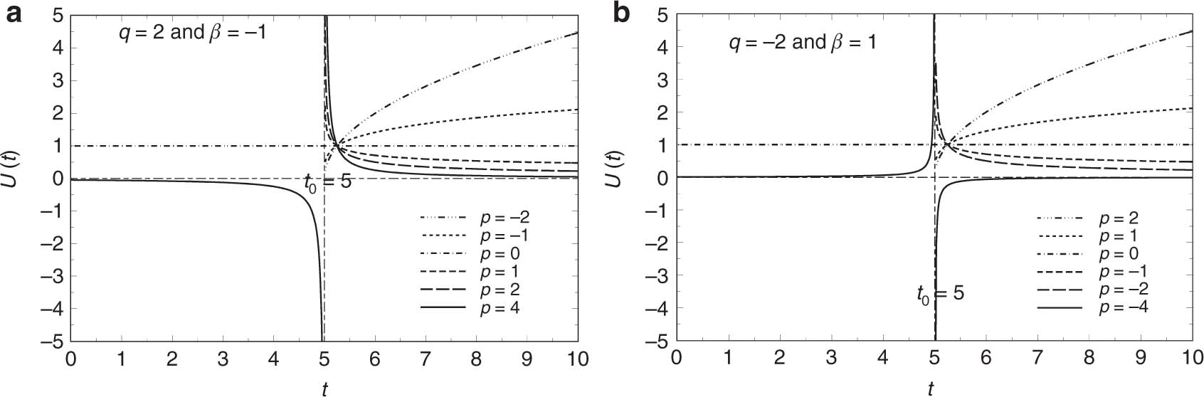
Temporal variation of the dimensionless plate velocity U(t) for various values of p when (a) q = 2 and β = −1 and (b) q = −2 and β = 1. For t > t₀, the plate velocity confirms the existence of the boundary layer flow either in p < or > 2q corresponding to β < or > 0. Here, the exceptional case is p = 0 for which the plate velocity is independent of time t.

6 Some Particular Cases

The self-similar solutions (15) and (16) for the boundary value problems (8) and (9) depend highly on the parametric values of M, p, q, and β, especially on the product values of qβ(<0). Here, we deduce the following two particular cases by considering the special values of these parameters.

1. For p = 0, qβ = −2, and M = 0, (8) and (9) reduce to the equations of the first Stokes problem of an infinite plane surface suddenly set into motion in its own plane with a uniform velocity U = 1 [1], p. 127].

2. For q = 0, (8) becomes a simple second-order linear ordinary differential equation, which provides us an analytic solution after using (9), as given below:

   (18)f(η)=e−pβ+M2η provided (pβ+M2)>0.

In addition with pβ = 1 and M = 0, the reduced form of (8) along with its solution (18) come to the same thing that was reported by Watson in his analysis [6], p. 359].

Thus, it can be confirmed that the above two results are the special cases of our present study, where we generalise the part ‘motion due to an infinite plane’ of the paper by Watson [7] as well as the first Stokes problem by incorporating the parameter β into the unsteady flow dynamics and extended these problems in the magnetic case. It is noticeable that (18) is the exact solution of the unsteady Navier–Stokes equations.

The surface shear stress τ_w is given by

The dimensionless surface shear stress, i.e. the skin-friction coefficient C_f(=τw/ρU02), is then obtained from (19) by using (11) and (12) as

From the outer boundary condition of (9), it is obvious that the fluid velocity f(η) becomes zero as η tends to infinity. Thus, the shear layer thickness δ₁ corresponds to the value of y, as such distance η_s of η where f(η) reached its limiting value (= 0.01, say). The non-dimensional shear layer thickness δ (=δ1U0/ν) is then obtained by using (15) and (16) as

Equation (21) accounts for the depth of penetration of the momentum to the fluid body. It is proportional to the square root of the product of qβ(<0) and t (t₀ < t < ∞). We note that for a large value of this product, δ tends to be infinity, the effect of which is the whole field above the plate surface eventually taking on the surface velocity. On the contrary, for small values of it, we will definitely get the boundary layer flow structure for this flow problem. Furthermore, for q = 0, we will always have the boundary layer flow character only when the condition in (18) is fulfilled.

7 Function Transformations

A suitable transformation of the function f(η) as f(η) = h(z) along with f′(η) = h˙(z) |qβ/2| and f′′(η)=h¨(z)|qβ/2|, where z=|qβ/2| η, can remodel the governing equation (8) [after using (10)] into the following forms:

For β > 0:

For β < 0:

where a dot denotes the derivative with respect to stretched (or compressed) variable z and p = 2α|q|. The corresponding boundary conditions are obtained as

For M = 0, (22), (23), and (26) corroborate with (20)–(22) in [7]. In this case, the above equations fail to show the influence of the unsteadiness parameter β on this flow dynamics, as they are free from β.

8 Analytic Solution and Critical Condition for Separation

An analytic solution is rare in the unsteady Navier–Stokes equations due to their inherent non-linearity. However, the self-similar (8), along with (9) and (10), conceives a closed-form analytic solution that is obtained in terms of the first kind confluent hypergeometric function F11(a;b;z) as

when the conditions qβ < 0, (pβ+M2)/2qβ≥0, and (pβ+qβ+M2)/2qβ gets a value greater than or equal to zero except (3/2) is satisfied. Here, f(η) satisfies the outer boundary condition at η = k. This implies that k is a large positive value (i.e. k → ∞), which is taken as 50 without any loss of generality. From (27), the wall velocity gradient f′(0) is obtained as follows:

When (pβ+qβ+M2)/2qβ=3/2, i.e. when pβ+M2=2qβ, we have F11(32;32;12qβk2)=e12qβk2→0 because qβ < 0 and k → ∞. This corresponds to a singularity in the solutions of the boundary layer equation as given in (27). Hence, for continuous solutions, we restrict ourselves to the values of p, q, and β in (pβ+qβ+M2)/2qβ<3/2, i.e. in (pβ+M2)<2qβ, which satisfies the condition as stated in (ii) in the non-magnetic case (M = 0). This relation confirms that the magnetic parameter increases the domain of continuous solution to this flow problem.

Also, for the special relation

equation (27) becomes the form

with

as F11(12;12;12qβη2)=e12qβη2 and F11(12;12;12qβk2)=0. It is well known that the separation within the flow appears for the vanishing wall shear stress, i.e. for f′(0)=0. Equations (31) as well as (28) ensure that f′(0)=0 for all non-zero values of p, q, and β, while M may or may not be zero. Most important, this result would not be materialised until (29) is satisfied. The relationship (29) is therefore called the critical condition of separation for this flow problem, from which one can easily obtain the critical value of any one of the physical parameters when the others are known and the corresponding velocity profile is called the separation profile.

Again, for p = 0, qβ = −2, and M = 0, we have the relations F11(0;12;−η2)=1 and erf(η)=2π∫0ηe−t2dt=2πηF11(12;32;−η2), which reduce (27) into the following form:

Equation (32) gives us the values of f′(0)=−2/π≈−1.12838 and the boundary layer thickness δ=2ηs(t−t0)=3.642772(t−t0). However, (32) is the same as that was obtained by Stokes in his analysis (see (5.97) in [1], p. 127]). Therefore, it may be concluded that the analytic solution (27) along with (28) can be used to investigate the problem considered in the present paper. However, we are not aware of any existing experimental data with which our present results may be compared.

9 Results and Discussion

The numerical results obtained from (27) and (28) for various values of the parameters p, q, β, and M are shown in the form of figures from which one can easily estimate the effects of these parameters on this flow field. We again notice that the parameters p and q are real but cannot be zero together. Therefore, we can discuss the central findings of this analysis in the three cases below.

9.1 Results for p = 0

Here, we consider only the zero value of p for which the plate surface moves with a constant velocity U (= 1), and consequently the fluid flow over the plate surface will be governed by the parameters q, β, and M. We note that the influence of q as well as β on these flow dynamics can be retrieved from the effect of qβ(<0). Increasing |qβ| when qβ < 0 is equivalent to either increasing q(>0) for a fixed negative value of β or increasing |β| when β < 0 for a fixed positive value of q. This indicates that such a two-parameter approach is needless and even misleading. However, to elucidate the gross effect of qβ(<0) on this flow field, we depict Figure 2, which displays the variation of f(η) with η for the non-magnetic case only. Here, we have considered the special value of qβ = −2 only to authenticate our numerical results as that presented by Stokes in his analysis. Velocity at a given position decreases steadily with an increase in |qβ| and consequently the shear layer thickness decreases. This result is closely associated with the change of scale of the distance in the y-direction, which diminishes continuously with an increasing value of |qβ| when qβ < 0 and resulting in the decrease of the fluid velocity inside the layer.

Figure 2:

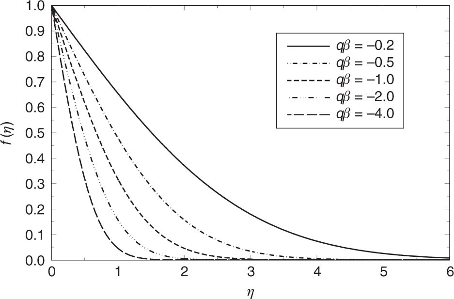
Variation of f(η) against η for various values of qβ(<0) when M = 0 and p = 0. The curve for qβ = −2 is the solution of the first Stokes problem. The velocity as well as the shear layer thickness decrease steadily with the increase in |qβ| when qβ < 0, owing to the decrease of the scale of the distance in the η-direction.

The effect of the externally applied magnetic field on the velocity profiles for a given value of qβ = −2 is shown in Figure 3. The velocity at a given position diminishes consistently as the strength of the magnetic field increases. This result ensures that the magnetic field has a strong influence on the fluid velocity even for all values of q and β when qβ(<0). Interestingly enough, the fluid velocity inside the layer is degraded faster at a large value of M with a low penetration into the fluid body. This result is physically significant and the physical reason behind such result is elucidated as follows. For an electrically conducting fluid, the influence of Lorentz force causes a loss of energy in the MHD flow owing to the complicated interaction between the flowing fluid and the electromagnetic field through the Lorentz force, introducing a significant amount of resistive force into this kind of flow problem. In fact, an increasing value of M is an implication of the more considerable influence of the Lorentz resistive force into the flow system. Thus, increase in M results in an increase of the magnitude of the wall velocity gradient, which, in turn, leads to decrease in the fluid velocity inside the layer that causes in the decrease of the penetration depth of the velocity field into the fluid body.

Figure 3:

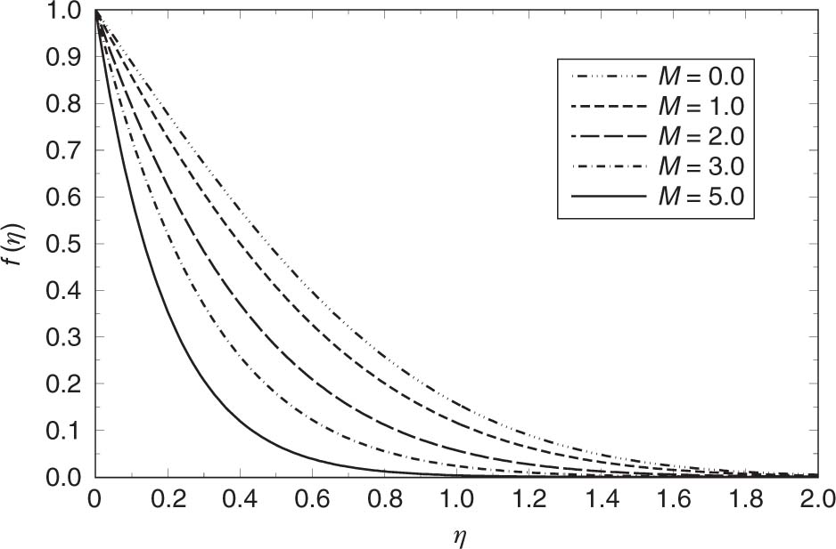
Variation of f(η) against η for various values of M when qβ = −2 and p = 0. The curve for M = 0 is the solution of the first Stokes problem. The maximum depth of penetration of the fluid flow is found in the absence of magnetic field.

9.2 Results for q = 0

For this special value of q (= 0), the plate velocity highly depends on time t, whereas the similarity variable η and the magnetic field B are completely free from that. Moreover, the governing boundary layer equation (8) visualises a closed-form analytic solution under a certain condition as given in (18). When M = 0, this condition strongly recommends the same sign of p and β, which means that pβ is always positive, whereas for non-zero values of M, they can also take values with opposite signs but up to a certain limit of the value of pβ(<0) for which the condition identified in (18) remains unchanged. It is perfectly understandable that the velocity f(η) will be decreased with an increasing value of pβ(>0) in both magnetic and non-magnetic cases. One more important point to note here is that the fluid velocity will be increased with an increasing value of |pβ| when pβ<0, only in the presence of a magnetic field. Thus, we see that there is no need to draw the figures in these perceptible cases.

In order to investigate the pivotal role of pβ(≠0) in combination with the magnetic parameter M on the velocity profiles, we have plotted the variation of f(η) against η for two dissimilar values of pβ (= −0.5 and 0.5) corresponding to three given values of M (= 0.8, 1.5, and 2.0) in Figure 4. For a fixed value of pβ, irrespective of its sign, the velocity at a given location decreases with the increase of M. Moreover, for a fixed value of M, the fluid velocity for any negative value of pβ is always higher than that of the same positive value of pβ, and this effect is more stringent for small values of (pβ+M2)>0. This stems from the fact that for a given non-zero value of M, the velocity gradient near the wall [i.e. f′(0)=−pβ+M2] increases continuously with an increasing value of |pβ| when pβ < 0, which, in turn, leads to increase in the fluid velocity inside the layer. Just the opposite result is true for pβ > 0. A small value of (pβ+M2) means the wall velocity gradient tends to be zero-minus (i.e. negative); however, it will never be zero owing to the condition as stated in (18). The novelty that arises from this figure [also from (18)] is that the velocity of the fluid flow tends to be zero in the limiting values of pβ and M (i.e. either for pβ → ∞ or M → ∞ or both). Thus, for a large value of M, a very thin layer of the fluid flow adjoining the plate surface will occur in any given value of pβ(≠0). Moreover, the largeness of M depends significantly on the values of pβ as a negative value of pβ thickens the layer, whereas a positive value of that does the reverse. Hence, we come to this conclusion that a well-suited boundary layer flow is possible by adjusting the suitable amounts of values of M and pβ. Finally, we can conclude that the magnetic field extends the domain of the analytic solution, as it can remove the restriction of sign (positive) on selecting the values of pβ but up to a certain limiting value of pβ(<0) depending upon the values of M.

Figure 4:

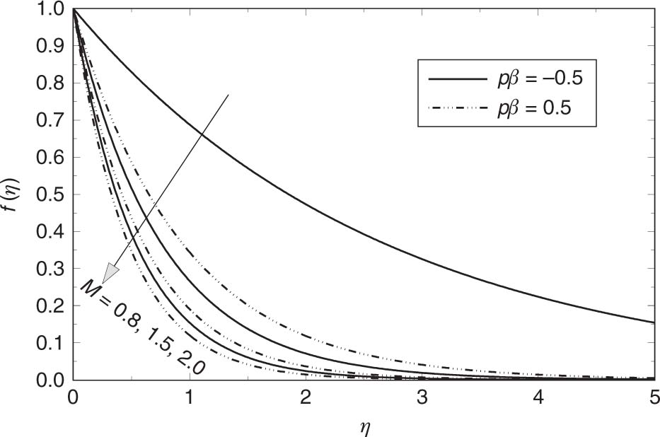
Variation of f(η) against η for two dissimilar values of pβ (= −0.5 and 0.5) corresponding to three fixed values of M (= 0.8, 1.5, and 2.0). The fluid velocity for a given value of pβ(>0) is always lower than that of the same negative numerical value of pβ as the wall velocity gradient (f′(0)=−pβ+M2) decreases continuously with an increasing value of pβ > 0.

From the above three examples (Figs. 2–4), it is clear that the effect of the parameters qβ(<0) and pβ(>0) is to reduce the fluid flow inside the layer, resulting in the increase of the magnitude of the wall velocity gradient. Moreover, the presence of the magnetic field enhances the effect of qβ(<0) as well as pβ(>0), and it also enlarges the solution domain by incorporating the negative values of pβ into the flow system. Here, the magnitude of the velocity gradient decreases with an increasing value of |pβ| when pβ < 0; however, it will never be zero owing to the condition in (18). Thus, we see that in the above two cases (Sections 9.1 and 9.2), there is no chance of getting a vanishing surface shear stress, the condition for the separation of flow inside the layer, for any given value of qβ(<0) and pβ in the presence as well as in the absence of the magnetic field. Hence, we can conclude that the solutions of the governing boundary layer equation (8) along with (9) and (10), especially for the above two cases, always have the boundary layer flow character without separation.

9.3 Results for Non-Zero Values of pand q

We have already discussed in detail the effects of the parameters qβ(<0) and pβ separately on this flow field by considering the special value of p = 0 and q = 0, respectively. We have found a continuous flow without separation inside the boundary layer after satisfying the condition in (18). This result is, however, no longer valid for all non-zero values of (p, q). In fact, separation appears inside the layer after a definite value of p depending upon the values of q and β. Moreover, the presence of the magnetic field suppresses the separation as well. This inspired us to examine the influence of magnetic field on this flow dynamics in addition to the non-zero values of (p, q), albeit following the conditions for the existence of the similarity solution as given in (i) and (ii).

Figure 5a demonstrates the variation of f′(0) versus p corresponding to three different values of q (= 0.5, 1 and 2) when β = −1 for both non-magnetic (M = 0) and magnetic (M = 2) cases. The surface shear stress, namely f′(0), increases steadily with an increase in p but up to the certain restricted value of p < (2qβ − M²)/β (= r, say), which satisfies the condition as stated in (ii) when M = 0. There exists a critical value p_c of p, dependent on q, β, and M, at which f′(0) becomes zero. Below this critical value, the surface shear stress is always negative and it decreases steadily with the decrease of p, however large p(<0) may be. Moreover, beyond this critical value, i.e. for p_c < p < r, the surface shear stress is always positive. The physical interpretation of these results is as follows. Here, the fluid flow is originated solely from the impulsive motion of an infinite plane surface moving with a velocity U(t) = C(t−t0)−γ, where C=(−2qβ)−γ and γ = p/2q. It ensures that for a given value of qβ (< 0) with q (> 0), the plate velocity will be increased with the increase of |p| when p < 0. This results in the enhancement of the dragging force of the plate surface on the fluid body, which, in turn, leads to decrease in the wall velocity gradient. Just the opposite clarification holds true for p(>0), so that the wall velocity gradient increases with an increasing value of p(>0) but up to the value of p < r. Owing to the decrease of the plate velocity with p(>0), the exerting force of the plate surface on the fluid body reduces and finally vanishes at a definite value of p within the range (0 < p < r). Indeed, it is the critical value of p(=pc) for which the flow separation appears inside the layer. However, after this critical value of p, the scenario of the dragging force changes dramatically, which means that the fluid body now exerts a dragging force on the plate surface. As a result, one must find the positive wall velocity gradient together with the flow separation inside the layer.

Figure 5:

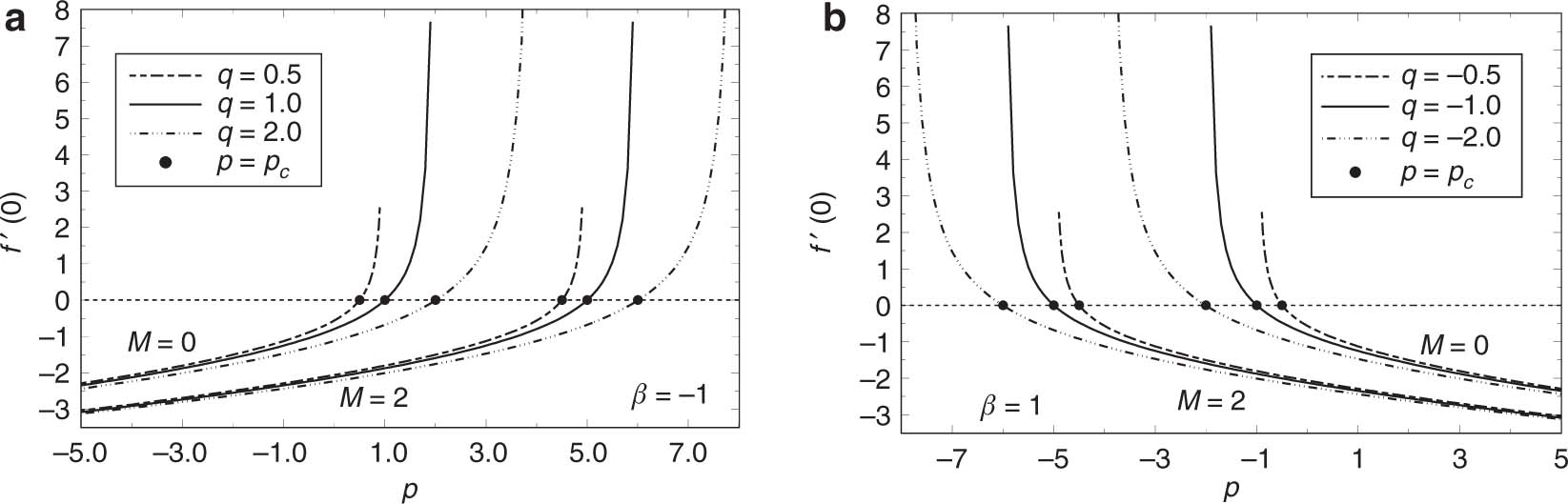
Variation of f′(0) with p at selected values of M and q when (a) β = −1 and (b) β = 1. The critical values p = p_c at which f′(0) vanish are indicated. The values of p_c can easily be obtained from (29). One figure is the mirror image of the other owing to the reflection symmetry of f: f(η,−p,q+,β−,M)=f(η,p,q−,β+,M).

Figure 5b shows the same variation along with the same values of qβ(<0) as used in Figure 5a when β = 1. It seems that the Figure 5b is a mirror image of Figure 5a. However, a closer look at these figures discloses the fact that the range of p (−∞ < p < r) for a fixed negative value of β is completely opposite (i.e. r < p < ∞) to the same positive numerical value of β. This is because the governing boundary layer equation (8) [after using (10)] conceives the reflection symmetry property: f(η,−p,q+,β−,M)=f(η,p,q−,β+,M), where the superscripts (+) and (−) denote the positive and negative values of the corresponding parameter, respectively. It is noticeable that the parameters q as well as M enlarge the solution domain by increasing the range of p with more negative velocity gradient at the wall, which, in turn, leads to delay in the separation inside the layer. Finally, we can conclude that the present flow field can be made more stable by considering the higher values of q and also by applying the high magnetic field into the system.

Here, the most important feature that comes into the view is the analytic solution (separation profile) under a certain condition (called the critical condition for separation) depending upon the non-zero values of (p, q) [see (29) and (30)]. However, from (29), it is easily discovered that the flow separation appears [f′(0) becomes zero] inside the layer at the value of p=(qβ−M2)/β. One can easily check that the critical values of p_c as indicated in Figure 5 are authenticated by this relation. Most important, this relation assures that in the non-magnetic case, the flow separation does not depend directly on the values of β; however, the value of q, whether positive or negative, depends completely on selecting the values of β as qβ < 0. Moreover, in this case, the flow separation arises at the value of p = q, whatever is the value of β. This feature is clearly shown in Figure 6a and b – one is the reflection symmetry of the other. Due to this reflection symmetry, we need to discuss the results with any one of them.

Figure 6:

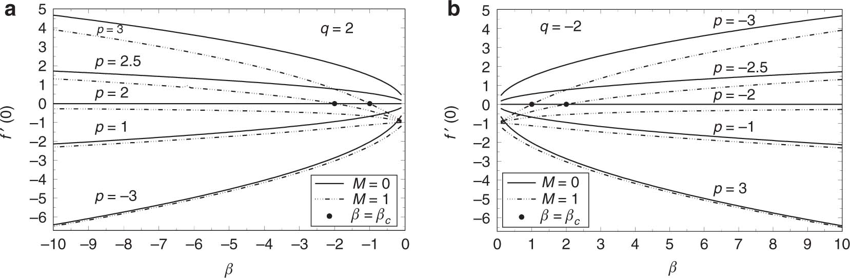
Variation of f′(0) against β at selected values of M and p when (a) q = 2 and (b) q = −2. The solid lines for p = q = 2 and p = q = −2 are the zero wall shear stress profiles for negative and positive values of β, respectively. The critical value β = β_c at which f′(0) vanishes in the presence of a magnetic field is indicated. The values of β_c validate the separation condition (29).

Figure 6a displays the variation of the surface shear stress f′(0) over the range (−10 ≤ β < 0) for several values of p when q = 2 in both the magnetic and non-magnetic cases. The surface shear stress is negative over the whole range of β(<0) only when p < q(=2=pc) for both cases, whereas it is positive in the non-magnetic case only for the values of p in (q < p < r). However, in the presence of a magnetic field, the velocity gradient for this range (q < p < r) may be either positive or negative depending on the values of β(<0). This implies the existence of a critical value of β, say β_c, as indicated in the figure, at which the wall velocity gradient is zero. Above this critical value, the velocity gradient is always negative and below this value it is positive. Here, the critical values of β for the curves p = 2.5 and 3 are β_c = −2 and −1, respectively. Obviously, for the fixed values of q and M, the critical value of β increases with the increase of p (> q). Further calculations reveal that for any given value of p in (q < p < r), the critical value β_c decreases rapidly with an increasing value of M. We note that the critical values of β_c rather agree with the separation condition as given in (29). Thus, we see that the magnetic field delays the flow separation, which indicates the more stable flow inside the layer. The stabilising effect of M on β(<0) is stringent for large positive values of p, whereas this effect is less significant for large negative values of p. This is because for the given values of p(<0) and q(>0), the plate velocity increases continuously with the increase of |β| when β < 0. Hence, the effect of a very large value of β(<0) in comparison with M leads the flow, and simultaneously the influence of a small value of M(=1) on this flow field will be insignificant. Finally, we can infer that the separation of the boundary layer flow can be removed completely by applying a proper amount of magnetic field strength M_c (say) depending upon the values of p, q, and β. As the value of p(>pc) increases, a high value of M_c is required to obtain the negative wall velocity gradient. This result is also true for the increasing value of |β| when β < 0. Just the opposite result is true for the increasing value of q (> 0). Most important, one should obtain the value of M_c by using the same condition as given in (29).

Owing to the reflection symmetry f(η,−p,q+,β−,M)=f(η,p,q−,β+,M), we only need to present the velocity profiles for q⁺ and β⁻. Figure 7a shows the similarity profiles f(η) with η for several values of p when q = 2, β = −1, and M = 0. The curve for p = 0 is the solution of the first Stokes problem. Here, we have taken the special value of p(=0) only to bring contrast to the variation of the boundary layer flows between negative and positive values of p as well. From this figure, it is clear that the velocity at a given location decreases with the increase of |p| when p < 0, and it increases with the increase of p(>0). The profile for p = 2 is the zero-wall-shear-stress profile (separation profile). Actually, it is the critical value of p (for the fixed values of q = 2 and M = 0) at which flow separation occurs. For any given value of p > 2, a reverse flow near the wall is observed in the variation of f(η). This is because the velocity gradient near the wall increases with an increasing value of p as the plate velocity decreases continuously with the increase of p, and this has already been explained in the discussion of Figure 5a.

Figure 7:

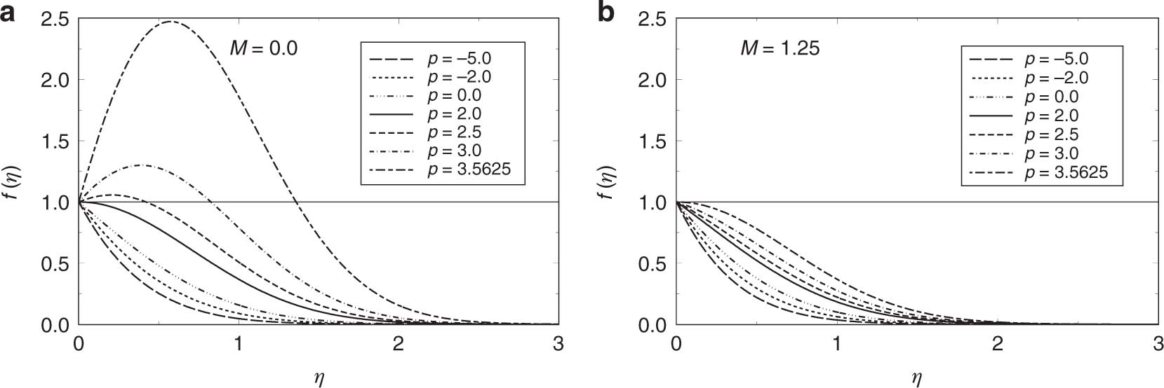
Variation of f(η) with η for several values of p(<2q) when q = 2 and β = −1 in (a) non-magnetic case (M = 0) and (b) magnetic case (M = 1.25). The profiles for p = 0 and 2 are, respectively, the profile of the first Stokes problem and the profile of separation in the non-magnetic case only. The profile for p = 3.5625 shows the reverse flow in the non-magnetic case, while it is the separation profile in the magnetic case.

Figure 7b displays the same variation along with the same values of p, q, and β as considered in Figure 7a for a fixed of M = 1.25, i.e. in the magnetic case. Here, the flow separation appears at a large value of p = 3.5625, in sharp contrast to the non-magnetic case where it occurred at the value of p = 2. The novelty that comes from the figure is that the reverse flow (which is exposed in the non-magnetic case; see Fig. 7a) can be completely removed by the use of a proper amount of magnetic field (M = 1.25), and we have pointed out such possibility earlier. Indeed, it is the critical value of M, which is obtainable from (29) when the other physical parameters are known (p = 3.5625, q = 2 and β = −1). Thus, we see that for a given value of p in (pc<p<r), there is a critical value of M below which the reverse flow always exists inside the layer and above that value no reverse flow occurs. This is because the externally applied magnetic field creates the Lorentz resistive force that tends to slow down the flow and essentially makes the boundary layer thinner. This thinning effect is more pronounced for higher values of M as well as decreasing values of p. This result is, however, true for the whole range of β(<0) in both magnetic and non-magnetic cases. This is demonstrated in Figure 8, which shows that the thinning effect of the magnetic field is more prominent for large positive values of p and small negative values of β. However, for the large negative values of β and for a given value of p, irrespective of its sign, the boundary layer thickness remains practically the same in both cases. This result is plausible and the physical reason for this fact is directly related to the fluid velocity within the layer.

Figure 8:

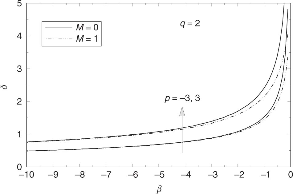
Variation of the dimensionless shear layer thickness δ against β(<0) for several values of M and p when q = 2. For any value of β < 0, shear layer thickness δ for a negative value of p is always lower than the same positive numerical value of p for both magnetic and non-magnetic cases.

We conclude our discussion by making some comments on this flow problem where the plate velocity is a function of time t and controlled by the parameters p and q. It is well known [1], p. 128] that the wall shear stress is negative when the plate is suddenly set into motion with a constant velocity in its own plane in an infinite mass of viscous fluid, which is otherwise at rest, i.e. for p = 0 in our present study. An outstanding result that emerges from our present study is that for any given value of q⁺, the plate velocity increases with the decrease of p⁻, whereas it decreases with the increase of p⁺ relative to its starting velocity (constant) at p = 0. Thus, we see that the present flow problem is accelerating or decelerating according to the values of p < or > 0. For accelerating flow, the plate surface always exerts a dragging force on the fluid body. As a result, the surface shear stress is always negative, which leads to the continuous flow inside the boundary layer. This implies that p⁻ has a powerful stabilising effect on these flow dynamics. This stabilisation effect is more pronounced with an increasing value of |p| when p < 0. For this reason, the present flow problem will continue even after a very large value of p⁻.

Conversely, the plate velocity continuously decreases from its starting velocity (i.e. the plate velocity for p = 0) with an increasing value of p⁺, resulting in an increase in the surface shear stress. This trend (negative surface shear stress) persists until we reach a certain critical value of p(=pc) at which the surface shear stress vanishes and flow separation occurs inside the layer. Interestingly enough, after this critical value of p(=pc), the surface shear stress is always positive. In this case, the boundary layer is divided into two regions: one is the reverse flow region [f(η) > 1 located from the wall to a finite range of η] and the other is the forward flow region, which approaches zero (free boundary condition) for very large values of η. The reverse flow zone increases with an increasing value of p⁺ (see Fig. 7). This suggests that the dragging force plays a vital role in controlling the behaviour of the flow structure over the plate surface. Physically, positive wall shear stress means that the fluid body exerts a dragging force on the plate surface owing to the deceleration of the surface velocity. This deceleration effect is pronounced with an increasing value of p⁺, and ultimately the plate velocity (and hence the fluid flow over the plate surface) dies out after a certain value of p⁺ depending upon the values of M and q⁺. Here, the key role of q⁺ is to reduce the value of p⁺, which leads to a delay in flow separation inside the layer.

10 Conclusion

A new class of similarity transformations, (15) and (16), have been devised for the unsteady laminar boundary layer flows of an electrically conducting viscous fluid over a flat plate moving in its own plane with a time-dependent velocity U(t). The conditions for the existence of the similarity solutions, essentially depending on the values of p, q, and β, are prescribed. The solution of the governing hydromagnetic equation (8) resulting from the suitably defined similarity variable in (15) is obtained in terms of the first kind confluent hypergeometric function F11(a;b;z). Our analysis is based on the solution of (8) in the limit of a low magnetic Reynolds number. We have examined in detail the influence of the parameters p, q, β, and M on the surface shear stress, given through f′(0) as well as on the similarity velocity profile f(η) of this flow problem. For p = 0, the current results are similar to the reported exact solution of the first Stokes problem. Furthermore, for q = 0, the governing hydromagnetic equation (8), provides us an analytic solution in a given condition (pβ+M2) > 0. The present analysis confirms that the surface shear stress is always negative in cases of both p = 0 and q = 0, where the results are the flow without separation. On the contrary, for non-zero values of (p, q), f′(0) can either be positive or negative, which depends on the values of p, q, β, and M. This indicates the existence of flow separation inside the boundary layer. The zero surface shear stress, which is the condition of flow separation, arises in the relation (pβ+M2=qβ). The most important feature of this study is the division of the existing solution range of p depending upon the separation criterion of vanishing wall shear stress. From this division criterion, one can easily recognise the possible flow behaviour (flow with or without separation) of this flow problem. Finally, we can conclude that the stabilising influence of the magnetic field plays an important role in making the flow stable by suppressing the reverse flow arising inside the layer.

Acknowledgement

The author is very grateful to the editors and referees for their valuable time spent on reading this paper. The author would also like to convey thanks to Mrs. A. Dholey and Dr. S. K. Garai for their kind cooperation during the work. This work was supported by the Science and Engineering Research Board (Funder Id: http://dx.doi.org/10.13039/501100001843, grant no. EMR/2016/005533) of India.

Nomenclature

A

real constant

B

magnetic field

C

dimensionless real positive constant

C_f

skin-friction coefficient

f

similarity function

g

an arbitrary function of time t

J

current density

k

positive constant

M

Hartmann number (magnetic parameter)

M_c

critical value of M

n

a real number

p, q

real numbers

p_c

critical value of p

q

fluid velocity vector

r

a real number =(2qβ−M2)/β

R_m

magnetic Reynolds number

t

time

t₀

constant reference value of t

u

fluid velocity in the x-direction

U

surface velocity

U₀

velocity scale

x, y

Cartesian coordinates

z

stretched (or compressed) variable

Greek symbols

β

unsteadiness parameter

γ

a real constant = p/2q

δ

dimensionless shear layer thickness

η

dimensionless distance normal to the plate surface

μ

dynamic coefficient of viscosity

μ₀

magnetic permeability

ν

kinematic coefficient of viscosity

ρ

fluid density

σ

electrical conductivity

τ_w

shear stress at the plate surface

Subscripts

c

critical

0

scale/reference value of the corresponding variable

w

surface (wall)

Superscripts

′

derivative with respect to η

˙

derivative with respect to t in Section 4

˙

derivative with respect to z in Section 7

⁻

dimensionless quantities

⁺

positive value of the corresponding parameter

⁻

negative value of the corresponding parameter

References

[1] H. Schlichting and K. Gersten, Boundary-Layer Theory, Springer-Verlag, New York 2000.10.1007/978-3-642-85829-1Suche in Google Scholar
[2] R. I. Panton, Incompressible Flow, Wiley, USA 1995.Suche in Google Scholar
[3] I. G. Currie, Fundamental Mechanics of Fluids, McGraw-Hill, New York 1993.Suche in Google Scholar
[4] F. M. White, Viscous Fluid Flow, McGraw-Hill, New York 1991.Suche in Google Scholar
[5] D. P. Telionis, Unsteady Viscous Flows, Springer, New York 1981.10.1007/978-3-642-88567-9Suche in Google Scholar
[6] L. Rosenhead, Laminar Boundary Layers, Clarendon Press, Oxford, UK 1963.Suche in Google Scholar
[7] E. J. Watson, Proc. R. Soc. Lond. A 231, 104 (1955).10.1098/rspa.1955.0159Suche in Google Scholar
[8] S. Dholey, Fluid Dyn. Res. 47, 1 (2015).10.1088/0169-5983/47/3/035504Suche in Google Scholar
[9] S. Dholey, Phys. Fluids 30, 1 (2018).10.1063/1.5022545Suche in Google Scholar
[10] S. Leibovich, J. Fluid Mech. 29, 401 (1967).10.1017/S0022112067000916Suche in Google Scholar
[11] J. Buckmaster, J. Fluid Mech. 38, 481 (1969).10.1017/S0022112069000292Suche in Google Scholar
[12] M. Katagiri, J. Phys. Soc. Jpn. 27, 1045 (1969).10.1143/JPSJ.27.1045Suche in Google Scholar
[13] M. Katagiri, J. Phys. Soc. Jpn. 27, 1662 (1969).10.1143/JPSJ.27.1662Suche in Google Scholar
[14] S. Dholey, ZAMM 96, 707 (2016).10.1002/zamm.201400218Suche in Google Scholar
[15] J. A. Shercliff, A Textbook in Magnetohydrodynamic, Pergamon Press, Oxford, UK 1965.Suche in Google Scholar
[16] V. J. Rossow, Phys. Fluids 3, 395 (1960).10.1063/1.1706048Suche in Google Scholar
[17] R. S. Nanda and A. K. Sundaram, ZAMM 13, 483 (1962).10.1007/BF01601075Suche in Google Scholar
[18] V. M. Soundalgekar, Appl. Sci. Res. 12, 151 (1965).10.1007/BF02923392Suche in Google Scholar
[19] I. Pop, Rev. Roum. Phys. 12, 865 (1967).Suche in Google Scholar
[20] C. Fetecau, R. Ellahi, M. Khan, and N. A. Shah, J. Porous Media 21, 589 (2018).10.1615/JPorMedia.v21.i7.20Suche in Google Scholar
[21] S. Dholey, Sadhana 44, 1 (2019).10.1007/s12046-018-0983-ySuche in Google Scholar
[22] S. Dholey and A. S. Gupta, Phys. Fluids 25, 1 (2013).10.1063/1.4788713Suche in Google Scholar
© 2020 Walter de Gruyter GmbH, Berlin/Boston
Artikel in diesem Heft
- Frontmatter
- Atomic, Molecular & Chemical Physics
- The Reaction and Microscopic Electron Properties from Dynamic Evolutions of Condensed-Phase RDX Under Shock Loading
- Trace Hydrogen Sulphide Gas Sensor Based on Cu/rGO Membrane-Coated Photonic Crystal Fibre Michelson Interferometer
- Dynamical Systems & Nonlinear Phenomena
- A General Viscous Model for Some Aspects of Tropical Cyclonic Winds
- Nonlinear Pull-in Instability of Rectangular Nanoplates Based on the Positive and Negative Second-Order Strain Gradient Theories with Various Edge Supports
- Hydrodynamics
- On the Heat Flow Through a Porous Tube Filled with Incompressible Viscous Fluid