A double clustering algorithm for financial time series based on extreme events

1 Introduction

In the analysis of the relationship between financial returns, the lower tail dependence quantifies the risk of investing on assets for which extremely negative returns could occur simultaneously. This is a very important issue for portfolio selection. Financial institutions have to offer to their customers the chance of investing money in a number of assets. But these assets should be poorly associated in the negative performances, in the sense that a fall in the quotations of an asset should not affect the quotations of the other assets. In order to have a measure of the association between two assets, some classical statistical tools are inadequate. The correlation coefficient is the main measure of association for quantitative data, but it has revealed its limit in this context. The correlation coefficient summarizes the linear relationship between two variables considering the entire probability distributions. However, in presence of non-linear relationships and when the interest is focused on the extremely low values of the variables, it is appropriate to adopt some specific association measures (see [16] for a comprehensive survey). In recent years literature has given much importance to the tail dependence, that is, the dependence between extreme values (see [18]). In particular, we can consider the upper tail dependence, when the interest lies in the very high values, and the lower tail dependence, when the interest is in the very low values.

Portfolio selection techniques are heavily affected by the estimated association of the potential assets. The classical approach has been designed by Markowitz [21] and is known as mean-variance approach (the resulting portfolio is known as mean-variance portfolio). Given n assets, the rationale of the mean-variance approach is that of choosing the weights of the assets, in such a way that the resulting portfolio has a specific expected value and the lowest possible variance. Since the variance is an indicator of the variability, and then of the risk, the solution of the Markowitz problem provides a diversified portfolio satisfying a fairly general criterion of minimization of the risk, based on linear correlation as association measure between returns. However, in the last decades a number of contributions has been presented in literature enriching the range of opportunities. Another measure of risk built on the entire distribution of the returns has been proposed by Bernardo and Ledoit [3], and later popularized by Keating and Shadwick [19] as Omega. A largely used alternative approach is the minimization of the Conditional Value-at-Risk (CVaR). The Value-at-Risk (VaR) is certainly the most popular measure of financial risk, largely used by financial institutions. It is defined as a threshold loss value, such that the loss on the portfolio over a given time horizon can exceed this value with a given (low) probability. The CVaR is the expected loss given that a loss greater than the VaR has occurred. The problem of minimizing the CVaR has been introduced by Rockafellar and Uryasev [24] and Krokhmal, Palmquist and Uryasev [20].

When the aim is the composition of a portfolio with low association in the extremely low values of the assets, the lower tail dependence coefficient has a dominant role. In [6] we have proposed to classify the assets in groups according to their association between very low returns, measured by the lower tail dependence coefficient. As a result, we have clusters composed of assets with a strong association between extremely low returns, while the assets belonging to different groups present a weak association between extremely low returns. The topic has been also faced by other authors. In [13], Durante, Pappadà and Torelli have proposed to carry out a clustering procedure based on the conditional Spearman’s correlation coefficient, and in [14] they have suggested a non-parametric estimation of the tail dependence coefficients, while in [12] Durante and Pappadà have clustered time series according to the pairwise Kendall distribution. A different approach has been studied by DiTraglia and Gerlach [11] exploiting a result from Extreme Value Theory to estimate the tail dependence and use it in portfolio selection.

The problem of time series clustering has also been explored in the literature from different perspectives; see, e.g., [23, 2, 5, 22, 15, 25, 4].

In terms of portfolio selection, we have introduced in [6] the strategy of picking one asset from each of the groups, such that the resulting portfolios are composed of assets with a low probability of a joint collapse. The weights of the selected assets are estimated using one of the known techniques. This research line has been further developed in [9] pursuing the idea that the lower tail dependence coefficients are not time-invariant, but have their own dynamics. As a result, the possible portfolios one can compose also change over time.

Up to now, the strategies proposed in this framework are designed to take into account only the dependence of returns in the lower tail, as it is considered the most crucial issue to prevent severe losses from occurring in financial crisis periods. In this paper we propose to go beyond this point and take into account the association of returns both in the lower and in the upper tail, so as to compose portfolios able to protect against crisis periods, while taking the best of booms. In detail, we present a development of the basic strategy ‘pick one asset from each cluster’, proposed in [6, 9]. More specifically, we propose to exploit the results of a second clusterization of the same assets based on the upper tail dependence coefficients. The idea is that of selecting assets which belong to different lower tail dependence-based clusters and, possibly, to a unique upper tail dependence-based cluster. If the last condition cannot be satisfied, we request to get as close as possible. In this case, for each possible selection derived from the lower tail dependence-based clusters, we compute the heterogeneity Gini index according to the position of the assets in the upper tail dependence-based clusters. At the end we opt for the selection which minimizes the Gini index. The rationale behind this strategy is that of selecting a well-diversified portfolio for crisis period that, at the same time, can take advantage of positive extreme events.

The paper is organized as follows. Section 2 describes the clustering procedure and presents the methods for finding the weights to compose a portfolio. In Section 3 the results of an extensive simulation study are illustrated. An application to a real dataset is discussed in Section 4 and, finally, Section 5 concludes.

2 Time series clustering on tail dependence

In this paper we refer to the clustering procedure proposed in [6], where time series of financial returns are clustered using a dissimilarity measure based on tail dependence coefficients, focusing either on the lower or on the upper tail. The dissimilarity measure is defined as

where {ri⁢t}t=1,…,T and {rj⁢t}t=1,…,T denote the time series of returns of two assets i and j, and λ^i⁢j is their estimated (lower or upper) tail dependence coefficient. For details about the estimation of tail dependence coefficients by means of copula functions, see [17, 16].

Given the time series of the returns of p assets, in the following we will denote by Λ^ the p×p symmetric matrix containing the (upper or lower) tail dependence coefficients between all the possible pairs of returns. The diagonal of Λ^ is composed of ones. Later, when we will need to distinguish between lower and upper tail dependence, the matrix will be denoted as Λ^L and Λ^U, respectively.

Given Λ^, the clustering procedure is composed of two steps. In step 1, starting from the dissimilarity matrix Δ^=(δ^i⁢j)i,j=1,…,p=-log⁡(Λ^), an optimal representation of the p time series {r1⁢t},…,{rp⁢t} as p points 𝐲1,…,𝐲p in ℝq is found by means of multidimensional scaling (MDS). The term optimal means that the Euclidean distance matrix D=(di⁢j)i,j=1,…,p, with di⁢j=∥𝐲i-𝐲j∥, of the p points 𝐲1,…,𝐲p in ℝq has to fit as closely as possible the dissimilarity matrix Δ^. The extent to which the interpoint distances di⁢j “match” the dissimilarities δ^i⁢j is measured by an index called stress, which should be as low as possible. The algorithm of MDS works for a given value of the dimension q, which has to be given in input. So, it is proposed to start with the dimension q=2 and then to repeat the analysis by increasing q until the minimum stress of the corresponding optimal configuration is lower than a given threshold s¯. In step 2, the p points 𝐲1,…,𝐲p in ℝq are clustered using a k-means algorithm. In [6] we have shown simulation studies where this two-step procedure outperforms the application of hierarchical clustering directly on the dissimilarity matrix Δ^. However, this is still an open issue. For example, Durante, Pappadà and Torelli [13, 14] propose a similar approach where the use of hierarchical clustering instead of the k-means algorithm allows them to avoid the MDS step.

The clusters obtained with this procedure are composed of assets characterized by high tail dependence in the (lower or upper) tail. We point out (see [6, 8, 7, 9]) that the clustering solution may be exploited for a preliminary decision about which stocks should be included in a portfolio. In other words, the idea is to use the clustering solution to select a small number of stocks to invest on, from among the p stocks available. Then, a portfolio is constructed by estimating proper weights using the common portfolio selection techniques (see Section 2.1).

When the clustering solution based on the lower tail is used, the selection is made by including in the portfolio assets belonging to different lower tail-based clusters, that allows to counterbalance possible extreme losses. On the other hand, the clustering solution based on the upper tail may be used, as well. In this case the opposite strategy should be followed: investing on assets belonging to the same upper tail-based cluster allows to take advantage of simultaneous extreme profits. In [6, 8, 7, 9] we have shown examples where portfolios including the stocks selected by means of lower tail-based clusters outperform the classical portfolio selection strategies. Instead, the performance of portfolios built relying on the upper tail-based clusters has not been explored so far, because the latest years financial situation suggested to protect from bears rather than take advantage of bulls.

In this paper we propose to select the stocks to include in the portfolio relying both on the lower tail-based and upper tail-based clusters. Again, a defensive approach is adopted, in the sense that the upper tail-based clusters are used as a second-best criterion to be exploited once the requirements based on the lower tail-based clusters have been fulfilled.

The proposed procedure is described in the next subsection.

3 Simulation study

In this section we describe the results of a simulation study investigating how the whole proposed procedure works. The main aim is to understand how effective the idea to exploit the clustering solution for portfolio selection is.

In Sections 3.1 and 3.2, we will describe the data generating process and the results obtained in the two phases, the clustering and the portfolio selection, of the proposed procedure.

As far as it concerns the data generating process, it is worth pointing out that to define a multivariate random variable able to allow different lower and upper tail dependence structures is a challenging task. Up to our knowledge, at the moment there is in the literature no procedure able to generate multivariate data with two (different) given matrices of lower and upper tail dependence coefficients. Some studies in this sense can be found in [1, 10], but they are not suited to the multivariate structure needed in this study. So, we will define a new random variable by joining two different multivariate Student-t variables, determining the behavior of the lower and the upper tail in a separate fashion.

In Section 3.2 the results of the portfolio selection are described, focusing on the out-of-sample performance of the proposed portfolios compared to two benchmark alternatives.

4 Empirical analysis of real data

Our procedure is applied to daily log-returns of the 50 stocks included in the EUROSTOXX index observed in the period from January 2, 2008 to December 31, 2013. The total number of returns for each stock is 1540. The EUROSTOXX index is designed to reflect the performance of the largest companies in the Eurozone and so is a measure of the performance of the financial markets in Europe.

Each time series of log-returns has been filtered to remove autocorrelation and heteroskedasticity by applying a univariate Student-t AR-GARCH models. The order of the autoregressive component ranges from 0 to 1, while for the heteroskedastic component the GARCH(1,1) model has provided a satisfactory fit for almost all the series (for a few time-series a GARCH(1,2) has been estimated). Then we have computed the distribution functions of the standardized residuals. Applying the Joe–Clayton copula, we obtain the 50×50 symmetric matrices containing the estimated lower and upper tail dependence coefficients, respectively Λ^L and Λ^U.

4.1 Clustering

Starting from Λ^L and Λ^U, we obtained the corresponding dissimilarity matrices Δ^L=-log⁡(Λ^L) and Δ^U=-log⁡(Λ^U). Then, we followed the procedure defined in Section 2.1. In doing that, we obtained the clustering as described in Section 2 two times, using firstly ΔL and secondly ΔU, in order to obtain, respectively, the two (lower tail-based and upper tail-based) clustering solutions G⁢L1,G⁢L2,…,G⁢LKL and G⁢U1,G⁢U2,…,G⁢UKU.

In order to select the optimal number of clusters, KL and KU, we inspected the graphs presented in Figure 1, displaying the pattern of the between over the total deviance and the corresponding increments, versus the number of clusters of the two clustering solutions.

Figure 1

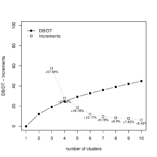
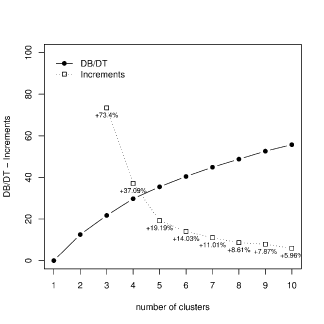
Ratio between deviance and total deviance: pattern and increments versus the number of clusters in the lower tail-based (left) and upper tail-based (right) clustering solutions.

We decided to set KL=5 and KU=6. The joint composition of the two clustering solutions is graphically summarized in Figure 2, where the five lower tail-based and the six upper tail-based clusters are represented respectively by columns and rows, while the squares contain the stocks belonging to the same cluster both in the lower tail-based and the upper tail-based solution.

Figure 2

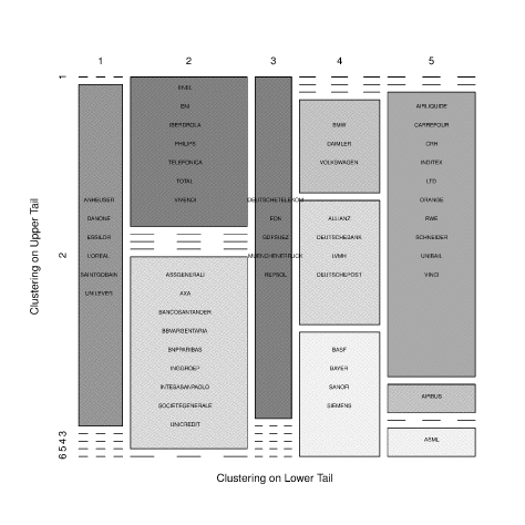
Joint composition of the clustering solutions G⁢L1,G⁢L2,G⁢L3,G⁢L4,G⁢L5 and G⁢U1,G⁢U2,G⁢U3,G⁢U4,G⁢U5,G⁢U6.

Step-by-step, the procedure described in Section 2.1 produced the following results:

1. First selection, based on G⁢L1,G⁢L2,G⁢L3,G⁢L4,G⁢L5: the cluster sizes were n1=6, n2=16, n3=5, n4=11, n5=12, so the set 𝐂(0) of the first-step candidates is composed of S(0)=63 360 possible portfolios of five stocks belonging to different clusters.

2. Second selection, based on G⁢U1,G⁢U2,G⁢U3,G⁢U4,G⁢U5,G⁢U6: the index γs was computed for each first-step candidate Cs(0); its minimum value was mins=1,2,…,63360⁡(γs)=0.768 and was reached by the 2.32% of first-step candidates. So, the set 𝐂 of second-step candidates is composed of S=1470 possible portfolios, selected from 𝐂(0) by taking into account the upper tail-based clustering solution. All the 1470 candidates are composed of five stocks belonging to different lower tail-based clusters and to three different upper tail-based clusters.

3. Final selection: the best portfolio among the 1470 second-step candidates is then chosen with financial criteria, as described in Section 4.2.

4.2 Portfolio selection

In detail, firstly the weights of the 1470 candidate portfolios are estimated by minimizing the CVaR, then the best portfolio is selected either with the minimum CVaR (portfolio C1) or the maximum Omega index criterion (portfolio C2), as described in Section 2.1. The performance of the selected portfolios has then been evaluated in an out-of-sample period, from January 1, 2014 to January 15, 2014 and compared to the two benchmark options considered in the simulation study (A: Markowitz minimum variance portfolio built using all the stocks; B: Minimum CVaR portfolio built using all the stocks).

Figure 3 shows the composition and the weights of the four analyzed portfolios. While portfolios C1 and C2 are composed of five stocks by construction, portfolios A and B turn out to be composed of eleven and nine stocks, respectively. In the specified out-of-sample period the cumulative returns of the four portfolios (with respect to December 31, 2013) are plotted in Figure 4. Portfolios C1 and C2 largely outperform the competitors. In the first four days, all the portfolios have a loss, but the lowest loss is always recorded for portfolio C1 (0.0070) while portfolio C2 is the second best except in the fourth day when its cumulative loss is slightly higher than the competitor portfolios. However, from the fifth to the tenth day, all the portfolios have positive returns, and the superiority of portfolios built using a clustering procedure is clear. At the sixth day, the cumulative returns of portfolios C1 and C2 are, respectively, 0.033 and 0.024 against 0.009 (portfolio A) and 0.010 (portfolio B). At the end of the out-of-sample period (15 January), the cumulative returns of portfolios C1 and C2 are 0.024 and 0.023, again much higher than portfolio A (0.013) and portfolio B (0.012).

Figure 3

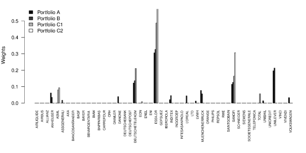
Weights of the stocks.

Figure 4

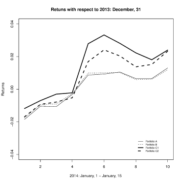
Returns of the portfolios.

5 Concluding remarks

In this paper a portfolio selection procedure has been proposed, taking into account the behavior of stock returns in case of extreme events, both negative and positive. The innovative proposal of this paper, with respect to previous work on this theme, is the idea of considering, beyond the lower tail of the distribution, also the upper tail. Specifically, the idea is to invest on stocks exhibiting, at the same time, low and high mutual association in case of, respectively, extremely low and extremely high returns. The association in case of extreme events is measured by (lower and upper) tail dependence coefficients estimated via copula functions. The portfolio selection is based on two preliminary time series clustering procedures, aimed at grouping together stocks with high (lower and upper) tail dependence. The two clustering solutions are jointly considered in order to provide a set of candidates portfolios and the “winner” of the competition is then chosen from among these candidates, using a financial criterion such as the minimum CVaR or the maximum Omega index. The definition of the set of candidate portfolios requires to consider the heterogeneity of all the possible portfolios than can be built relying on one clusterization, with respect to the other. For this reason, the computation burden implied by the proposed procedure tends to grow rapidly as the number of considered stocks increases. Then, the method cannot realistically be applied to very large sets of stocks.

The performance of the procedure has been successfully checked on simulated data, with an experiment aimed at verifying (i) the adequateness of copula functions estimation of the tail dependence structure with a misspecified distributional assumption, (ii) the ability of the procedure in recovering the right clustering structures, and (iii) the comparison of the selected portfolios’ returns to those obtained by two common portfolio selection techniques, used as benchmarks.

Finally, a case study on real data from the EUROSTOXX index shows that the portfolios selected according the proposed procedure have been able to outperform the benchmarks in a two-weeks out-of-sample period.

References

[1] K. Aas, C. Czado, A. Frigessi and H. Bakken, Pair-copula constructions of multiple dependence, Insurance Math. Econom. 44 (2009), 182–198. 10.1016/j.insmatheco.2007.02.001Suche in Google Scholar
[2] A. M. Alonso, J. R. Berrendero, A. Hernández and A. Justel, Time series clustering based on forecast densities, Comput. Stat. Data Anal. 51 (2006), 762–776. 10.1016/j.csda.2006.04.035Suche in Google Scholar
[3] A. Bernardo and O. Ledoit, Gain, loss and asset pricing, J. Political Econom. 108 (2000), 144–172. 10.1086/262114Suche in Google Scholar
[4] W.-C. Chen and R. Maitra, Model-based clustering of regression time series data via APECM. An AECM algorithm sung to an even faster beat, Stat. Anal. Data Min. 4 (2011), 567–578. 10.1002/sam.10143Suche in Google Scholar
[5] M. Corduas and D. Piccolo, Time series clustering and classification by the autoregressive metrics, Comput. Stat. Data Anal. 52 (2008), 1860–1872. 10.1016/j.csda.2007.06.001Suche in Google Scholar
[6] G. De Luca and P. Zuccolotto, A tail dependence-based dissimilarity measure for financial time series clustering, Adv. Class. Data Anal. 5 (2011), 323–340. 10.1007/s11634-011-0098-3Suche in Google Scholar
[7] G. De Luca and P. Zuccolotto, Dynamic clustering of financial assets, Analysis and Modeling of Complex Data in Behavioural and Social Sciences, Springer, Berlin (2014), 103–111. 10.1007/978-3-319-06692-9_12Suche in Google Scholar
[8] G. De Luca and P. Zuccolotto, Time series clustering on lower tail dependence for portfolio selection, Mathematical and Statistical Methods for Actuarial Sciences and Finance, Springer, Berlin (2014), 131–140. 10.1007/978-3-319-02499-8_12Suche in Google Scholar
[9] G. De Luca and P. Zuccolotto, Dynamic tail dependence clustering of financial time series, Stat. Papers (2015), 10.1007/s00362-015-0718-7. 10.1007/s00362-015-0718-7Suche in Google Scholar
[10] E. Di Bernardino and D. Rullière, On tail dependence coefficients of transformed multivariate Archimedean copulas, Fuzzy Sets and Systems 284 (2016), 89–112. 10.1016/j.fss.2015.08.030Suche in Google Scholar
[11] F. J. DiTraglia and J. R. Gerlach, Portfolio selection: An extreme value approach, J. Banking Finance 37 (2013), 305–323. 10.1016/j.jbankfin.2012.08.022Suche in Google Scholar
[12] F. Durante and R. Pappadà, Cluster analysis of time series via Kendall distribution, Adv. Intell. Syst. Comput. 315 (2015), 209–216. 10.1007/978-3-319-10765-3_25Suche in Google Scholar
[13] F. Durante, R. Pappadà and N. Torelli, Clustering of financial time series in risky scenarios, Adv. Data Anal. Class. 8 (2014), 359–376. 10.1007/s11634-013-0160-4Suche in Google Scholar
[14] F. Durante, R. Pappadà and N. Torelli, Clustering of time series via non-parametric tail dependence estimation, Stat. Papers 56 (2015), 701–721. 10.1007/s00362-014-0605-7Suche in Google Scholar
[15] P. D’Urso and E. A. Maharaj, Autocorrelation-based fuzzy clustering of time series, Fuzzy Sets and Systems 160 (2009), 3565–3589. 10.1016/j.fss.2009.04.013Suche in Google Scholar
[16] J. Franke, W. Härdle and C. Hafner, Statistics of Financial Markets: An Introduction, 4th ed., Springer, Berlin, 2015. 10.1007/978-3-642-54539-9Suche in Google Scholar
[17] W. Härdle, N. Hautsch and L. Overbeck, Applied Quantitative Finance, 2nd ed., Springer, Berlin, 2009. 10.1007/978-3-540-69179-2Suche in Google Scholar
[18] H. Joe, Multivariate Models and Dependence Concept, Chapman & Hall, New York, 1997. 10.1201/9780367803896Suche in Google Scholar
[19] C. Keating and W. Shadwick, A universal performance measure, J. Perform. Measur. 6 (2002), 59–84. Suche in Google Scholar
[20] P. Krokhmal, J. Palmquist and S. Uryasev, Portfolio optimization with conditional value-at-risk objective and constraints, J. Risk 4 (2002), 43–68. 10.21314/JOR.2002.057Suche in Google Scholar
[21] H. Markowitz, Portfolio selection, J. Finance 7 (1952), 77–91. 10.12987/9780300191677Suche in Google Scholar
[22] E. Otranto, Clustering heteroskedastic time series by model-based procedures, Comput. Stat. Data Anal. 52 (2008), 4685–4698. 10.1016/j.csda.2008.03.020Suche in Google Scholar
[23] F. Pattarin, S. Paterlini and T. Minerva, Clustering financial time series: An application to mutual funds style analysis, Comput. Stat. Data Anal. 47 (2004), 353–372. 10.1016/j.csda.2003.11.009Suche in Google Scholar
[24] R. T. Rockafellar and S. Uryasev, Optimization of conditional value-at-risk, J. Risk 2 (2000), 21–41. 10.21314/JOR.2000.038Suche in Google Scholar
[25] J. A. Vilar, A. M. Alonso and J. M. Vilar, Non-linear time series clustering based on non-parametric forecast densities, Comput. Stat. Data Anal. 54 (2010), 2850–2865. 10.1016/j.csda.2009.02.015Suche in Google Scholar
© 2017 Walter de Gruyter GmbH, Berlin/Boston
Artikel in diesem Heft