Introduction to the dynamical properties of Toeplitz operators on the Hardy space of the unit disc
-
Emmanuel Fricain
 und
Maëva Ostermann
und
Maëva Ostermann

Abstract
These notes are based on a mini-course given at the ACOTCA conference 2025. The goal is to present full proofs of the first two key results regarding hypercyclic Toeplitz operators, in a way that is accessible to beginners.
1 Introduction
These notes are based on a short mini-course, consisting of three 50-min lectures, which the fist author delivered at the ACOTCA (XIX Advanced Course in Operator Theory and Complex Analysis) held in June 2025 in Clermont-Ferrand, France. The topic concerns the hypercyclicity of Toeplitz operators on the Hardy space H
2 of the open unit disc
These notes are intended neither as a comprehensive survey of the literature on this subject nor as a presentation of new results. Rather, their purpose is to provide an introductory account accessible to readers approaching the topic for the first time. To this end, the exposition is aimed at readers (participants) with a background corresponding to a standard master’s level course in functional analysis and complex analysis and includes complete proofs of most of the results discussed.
The central question addressed in these notes is the following: given a function
The structure of this mini-course is as follows. Lecture 1 (Section 2) provides a brief introduction to the notion of hypercyclicity, restricted to the tools required for our purposes. In particular, we establish the classical Godefroy–Shapiro criterion and recall some basic and well-known obstructions to hypercyclicity. Lecture 2 (Section 3) contains a concise introduction to Hardy spaces and Toeplitz operators. Lecture 3 (Section 4) is devoted to the main question under consideration. Our discussion will focus on two fundamental results: the first one, due to Godefroy and Shapiro, characterizes hypercyclic Toeplitz operators with anti-analytic symbols; the second one, due to Shkarin, concerns tridiagonal Toeplitz operators. As will become apparent, even in this last restricted setting, the problem remains far from straightforward. The paper concludes with a brief mention of three more recent contributions to the study of hypercyclicity for Toeplitz operators.
To close this introduction, let us emphasize that the question of hypercyclicity for Toeplitz operators remains far from being completely resolved, and significant challenges persist. In particular, in [1], you could find some more specific open problems. We hope that these notes will motivate interested readers to pursue further investigation into this topic.
2 Hypercyclic operators
2.1 Definition of hypercyclicity
We usually imagine chaos as something that arises in nonlinear systems, while linear systems are thought to be predictable and “well-behaved”. But this intuition is not always correct. In fact, some natural linear operators can behave in a surprisingly chaotic way. One of their key features is the existence of a dense orbit: starting from a single point and repeatedly applying the operator, the trajectory can come arbitrarily close to every point in the space.
Definition 2.1.
More formally, let X be a Fréchet space, that is a complete topological vector space whose topology is generated by a countable family of seminorms, and let T: X → X be a continuous and linear operator on X (in short
is dense in X. In such a case, x is called a hypercyclic vector for T and the set of all hypercyclic vectors for T is denoted by HC(T).
Example 2.2.
The first known example of a hypercyclic operator was constructed by Birkhoff in 1929 [2], illustrating that such “chaotic” behavior can indeed occur even for linear operators. Let
Then T
a
is hypercyclic on
Example 2.3.
Another early example of a hypercyclic operator, still on the Fréchet space
Example 2.4.
On Banach spaces, the first known example is provided by Rolewicz in 1969 [4]. Let
Then λT is hypercyclic on X if and only if |λ| > 1.
Inspired by these early examples, researchers in the 1980s started studying the dynamical behavior of general linear operators, paying special attention to the phenomenon of hypercyclicity. This marked the beginning of a systematic exploration of “chaotic” behavior in linear settings. Some classical references for this area of research include:
Erdmann – Peris, “Linear Chaos”, 2011 [5];
Bayart – Matheron, “Dynamics of linear operators”, 2009 [6].
In particular, these references contain all the results discussed in this section, and we draw on them as a source of inspiration for this brief introduction to hypercyclicity.
2.2 Birkhoff’s transitivity theorem and Godefroy Shapiro criterion
The most useful characterization of hypercyclicity is an application of the Baire category theorem and is due to Birkhoff through the notion of topological transitivity. We first recall this notion.
Definition 2.5.
Let X be a Fréchet space and
Theorem 2.6
(Birkhoff’s transitivity theorem, 1922 [7]). Let X be a separable Fréchet space and
T is hypercyclic;
T is topologically transitive.
See Figure 1 for an illustration of the notion of topological transitivity.
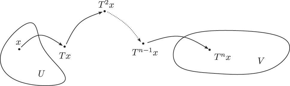
Topological transitivity.
Proof.
(i) ⇒ (ii): Assume that T is hypercyclic and let x be a hypercyclic vector for T. Consider U and V be two non-empty open sets of X. Since orb(T, x) is dense in X, there is some k ≥ 0 such that T k x ∈ U. But the space X has no isolated points, and then the set {T m x; m ≥ k} is also dense in X. Hence there exists m ≥ k such that T m x ∈ V. Observe now that
meaning that T n (U) ∩ V ≠ ∅ with n = m − k. Thus T is topologically transitive.
(ii) ⇒ (i): Assume now on the contrary that T is topologically transitive and let us prove that T is hypercyclic. Since X has a countable dense set {y
j
; j ≥ 1} (remember that X is separable), then the open balls of radius 1/m around the y
j
, j, m ≥ 1, form a countable base
By continuity of T, the sets
are open sets for every k ≥ 1. Let’s prove that W k is dense for every k ≥ 1.
Let U be an open set of X. Since T is topologically transitive, there exists n ≥ 0 such that
Therefore W
k
is dense in X. By Baire category theorem, the set
Remark 2.7.
Let
and to apply Birkhoff theorem.
As was observed by Godefroy and Shapiro, it turns out that if an operator has sufficiently many eigenvectors, then it is hypercyclic.
Theorem 2.8
(Godefroy – Shapiro citerion, 1991 [8]). Let X be a separable Fréchet space and
are dense in X. Then T is hypercyclic on X.
Proof.
We shall prove that T is topologically transitive. Let U and V be two non-empty open subsets of X. By assumption, U ∩ H −(T) ≠ ∅ and V ∩ H +(T) ≠ ∅. In other words, we can find
with Tx
k
= λ
k
x
k
with |λ
k
| < 1, Ty
k
= μ
k
y
k
with |μ
k
| > 1 and
and
Taking into account the fact that U and V are open subsets, it follows that there is some
In other words, V ∩ T n (U) ≠ ∅ meaning that T is topologically transitive. According to Birkhoff’s theorem, we then deduce that T is hypercyclic.□
2.3 Some restrictions to hypercyclicity
We assume now that X is a complex separable Banach space.
Proposition 2.9.
Let
Proof.
Let x ∈ HC(T) and argue by contradiction assuming that T*(x*) = μx* for some
Observe that the set
Proposition 2.10.
Let
If ‖T‖ ≤ 1 then T is not hypercyclic on X.
If for every x ∈ X, ‖Tx‖ ≥ ‖x‖, then T is not hypercyclic on X.
Proof.
(a) If ‖T‖ ≤ 1, then for every x ∈ X and every n ≥ 1, we have ‖T n x‖ ≤ ‖x‖. Hence the orbit orb(T, x) is bounded, and then cannot be dense in X. Since this is true for every x ∈ X, then T is not hypercyclic.
(b) If for every x ∈ X, ‖Tx‖ ≥ ‖x‖, then for every x ∈ X and every n ≥ 0, we have ‖T n x‖ ≥ ‖x‖. Hence the orbit orb(T, x) stays away from 0 (if x ≠ 0) and then cannot be dense in X. One more time, T cannot be hypercyclic on X.□
In the context of Hilbert spaces, we will show that a hyponormal operator cannot be hypercyclic.
Definition 2.11.
Let H be a Hilbert space and
Fact 2.12.
If T is hyponormal, then we have
Proof.
Write:
□
Theorem 2.13.
Let
Proof.
Let x ∈ H, x ≠ 0.
Assume first that the sequence
Now, it remains to prove that when the sequence
By assumption, there exists
An induction shows that
We finish this first lecture (section) by giving some spectral restrictions.
Theorem 2.14.
Let X be a complex separable Banach space and
Proof.
We argue by contradiction and suppose that
If
which contradicts the fact that T is hypercyclic.
If
Therefore
But it is not difficult to see that
Kitai proved indeed a better result.
Theorem 2.15
(Kitai, 1982 [9]). Let X be a complex separable Banach space and
3 Toeplitz operators and Hardy spaces
3.1 Toeplitz matrices
Recall that a Toeplitz matrix on
where
Let
Let
Note that
where
is a unitary operator.
Hartman and Wintner in 1954 got a characterization of the Toeplitz matrices that give rise to bounded operators on
Theorem 3.1
(Hartman – Wintner, 1954 [10]). The following assertions are equivalent:
The operator T(a) is bounded on
There exists a function
Moreover, UT(a)U −1 = T ϕ , where T ϕ f = P +(ϕf) f ∈ H 2.
Proof of (ii) ⟹ (i).
First note that if
Hence T ϕ is bounded on H 2 and ‖T ϕ ‖ ≤ ‖ϕ‖∞.
Moreover, let
Hence, for every n, k ≥ 0, we have
For the proof of (i) ⟹ (ii), we refer to the following book: “An introduction to operators on the Hardy-Hilbert space” by Rubén A. Martinez-Avendaño and Peter Rosenthal, 2007 [11].□
We will now discuss basic properties of Toeplitz operators T
ϕ
on H
2 when the symbol
3.2 The Hardy space H 2
The space H
2 can be identified with the space
where Taylor coefficients
where
is a unitary operator and
Using Parseval equality, it is not difficult to see that if f
r
(eiθ
) = f(reiθ
), 0 ≤ r < 1,
In particular, there exists a sequence
In fact, a deep result of Fatou says much more: if
where nt − lim denotes the non-tangential limit, that is the limit restricted to every Stolz region Δ α (see Figure 2).
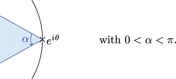
A Stolz region.
In the sequel, we will identify, as usual, H
2 and
Indeed, we have
3.3 Toeplitz operators on H 2
If we come back to Toeplitz operators on H 2, we have the following result on the norm.
Theorem 3.2
(Brown – Halmos, 1963 [12]). Let
Proof.
We have already seen that T ϕ is bounded and ‖T ϕ ‖ ≤ ‖ϕ‖∞.
For the converse inequality, denote by
Moreover, using that
where
We will now use a well-known property of the Poisson integral (see [11], Corollary 1.1.27]) saying that
Hence, according to [7], it follows that for almost all
Hence ‖ϕ‖∞ ≤ ‖T ϕ ‖, which concludes the proof.□
Some observations.
Let ϕ ∈ L ∞. It is easy to see that
If ϕ ∈ H ∞, the algebra of bounded and analytic functions on
Indeed, let f ∈ H 2, then
Now observe that since ϕ ∈ H ∞, then ϕf ∈ H 2 and we deduce that
Therefore,
In general, T ϕ T ψ ≠ T ϕψ but Brown and Halmos proved the following.□
Theorem 3.3
(Brown – Halmos, 1963 [12]). Let
We will do not really use this result so we will admit it. However, note that, in general, we have
As we have seen in the first part, the question of eigenvectors is crucial in the study of hypercyclicity. We will now give two results in this direction.
Theorem 3.4
(Coburn, 1966 [13]). Let
Proof.
Argue by contradiction and assume that there are two functions h
1 and h
2 in H
∞, h
1, h
2 ≠ 0 such that T
ϕ
h
1 = 0 and
Let now define
When the symbol ϕ is continuous, we can link the spectral properties of T
ϕ
with the winding number of ϕ. Recall that if
Furthermore, recall that an operator
Im(T) is closed;
ker(T) and ker(T*) are both finite dimensional.
In this case, the index of T is defined as
When ϕ is continuous, we have the following description of the spectrum.
Theorem 3.5.
Let
T ϕ is a Fredholm operator on H 2 if and only if ϕ does not vanish on
We have
This beautiful theorem is the combined work of several mathematicians: Krein, Calderón, Spitzer, Widom, Devinatz. Since we will not really use this result in the sequel, we will admit it. However, we refer to the book of Martinez-Avendaño – Rosenthal [11] for its proof and more details.
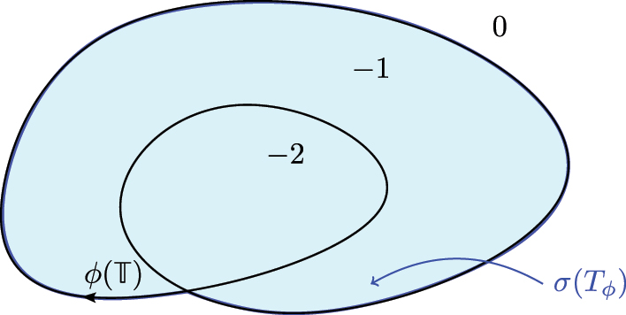
The spectrum of a Toeplitz operator.
Observe that if
so, we necessary have dimker(T ϕ − λ) > 0. Hence
and
Example 3.6.
If S denotes the shift operator on H 2, it can be easily proved that
Let ϕ be a continuous symbol such that
4 Hypercyclicity of Toeplitz operators
Recall that we are interested in the following question: given a function
4.1 Analytic and anti-analytic symbols
We start with a simple observation. If ϕ ∈ H
∞, then T
ϕ
is not hypercyclic on H
2. Indeed, since ϕ ∈ H
∞, then for every
(see [2]) and in particular
The case of anti-analytic symbol was studied by Godefroy and Shapiro.
Theorem 4.1
(Godefroy – Shapiro, 1991 [8]). Let ϕ ∈ H ∞. The following assumptions are equivalent.
ϕ is non-constant and
Proof.
(ii) ⟹ (i). Since ϕ is non constant, by the open mapping theorem,
Let
where we recall that
According to Godefroy – Shapiro Criterion, it is sufficient to prove that if Ω is a non empty open subset of
But since Ω is a non-empty open subset of
(i) ⟹ (ii). Assume now that
Now, a simple connectedness argument implies that
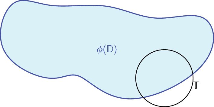
Hypercyclic operator.
We immediately recover the result of Rolewicz.
Corollary 4.2
(Rolewicz, 1969 [4]). Let
4.2 Tridiagonal Toeplitz operators
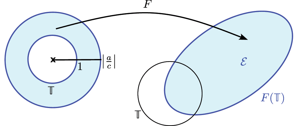
In [14], Shkarin characterized hypercyclic Toeplitz operators T F with symbols of the form
They correspond to the following Toeplitz matrices which are tridiagonal.
Observe that T
F
= aS* + bI + cS and then
Since S* is a contraction, we have I − SS* ≥ 0. Thus if |c| ≥ |a|, we get
Thus we may assume that |c| < |a|. We need now two lemmas.
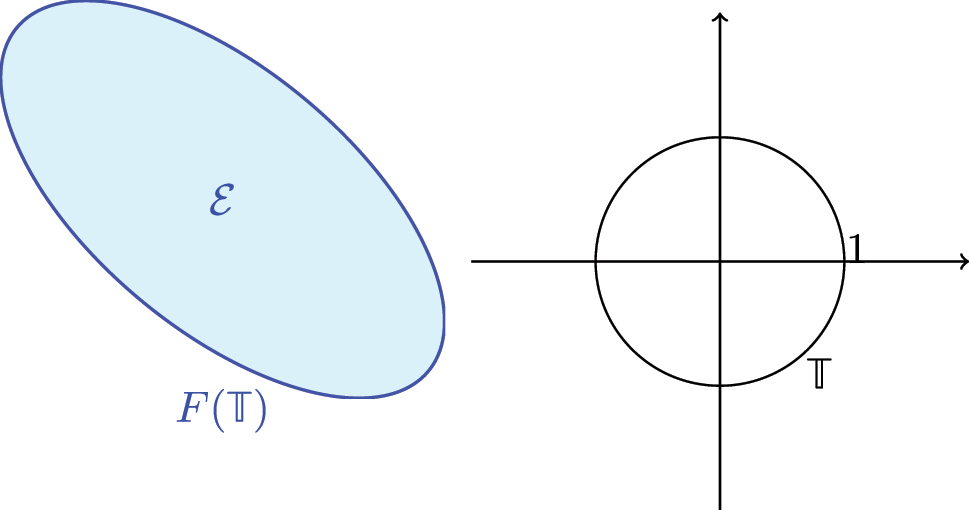
Lemma 4.3.
Let
The interior
See Figure 5.
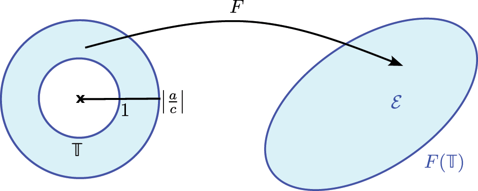
Shkarin Toeplitz operators.
Proof.
Let a = |a|eiα
, c = |c|eiγ
and consider
This formula shows that we can assume, without loss of generality, that b = 0 and a and c are real with a > c > 0.
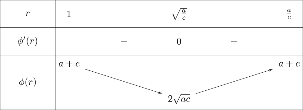
(a) F(eiθ ) = ae−iθ + ceiθ = (a + c)cosθ + i(c − a)sinθ. Hence
and thus
(b) We have
Let us first check that
If we denote by
Hence for all
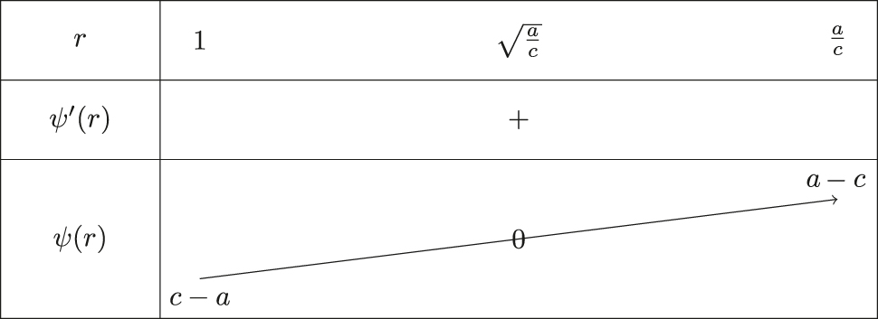
Hence for all
which means that
Let us now check that
Let
Observe that
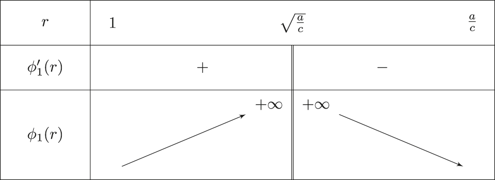
Moreover
Now, we can find
Hence
□
Lemma 4.4.
Let
Assume that A has an accumulation point in W (see Figure 6). Let
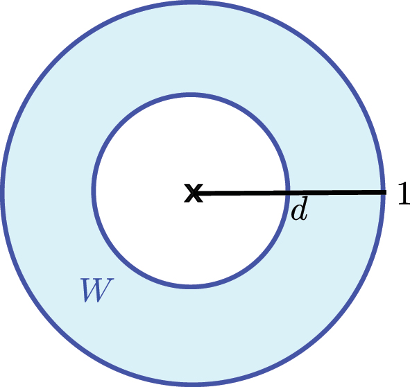
The annulus W.
Proof.
Observe that z⟼q(z) and
Then
Hence
We can now give the Shkarin’s characterization for hypercyclicity of tridiagonal Toeplitz operators.
Theorem 4.5
(Shkarin, 2012 [14]). Let F(eiθ
) = ae−iθ
+ b + ceiθ
, where
T F is hypercyclic on H 2;
the following two conditions are satisfied:
|a| > |c|;
Proof.
(1) ⟹ (2): let us first assume that T
F
is hypercyclic on H
2. We have already seen that (i) is necessary (because if |a| ≤ |c|, then T
F
is hyponormal and hence not hypercyclic). Let us now check (ii). Argue by contradiction and assume that
We have
Hence, there exists
Hence, by Cauchy–Schwartz’ inequality, we get
(2) ⟹ (1): let us now assume that (i) and (ii) are satisfied and let us check that T
F
is hypercyclic on H
2. By Lemma 4.3, we know that
See Figure 8.
We are going to prove that every point in
Now observe that
and since
belongs to H 2. Thus
where μ = F(z
0) and
By Godefroy – Shapiro Criterion, it is sufficient to check that if Ω is a non empty open set of
So let h ∈ H 2 such that for every z 0 ∈ Ω, we have
Note that if
where we recall that k
w
denotes the reproducing kernel at w of H
2 (observe that
Thus for every z
0 ∈ Ω with
Denote by
Non hypercyclic Toeplitz operator.
Hypercyclic Toeplitz operator.
4.3 Some more recent results
To go a little bit further, we conclude by mentioning three recent papers.
The first one is by Baranov – Lishanskii, 2016 [15]. They investigate the more general case where F has the form
where P is an analytic polynomial and
where R is a rational function without poles in
Finally, using the model theory for Toeplitz operators with smooth symbols developed by D. Yakubovich in the 80s, Fricain – Grivaux – Ostermann obtained in [1] some new necessary and sufficient conditions for Toeplitz operators to be hypercyclic on H
p
, 1 < p < ∞. We will take some time to discuss the flavor of some results obtained in [1]. Let q be the conjugate exponent of p, that is
F belongs to the class
the curve
F is injective on the interior of each arc α j , 1 ≤ j ≤ m;
for every i ≠ j, 1 ≤ i, j ≤ m, the sets F(α j ) and F(α j ) have disjoint interiors;
for every
Recall that
Theorem 4.6
(Fricain – Grivaux – Ostermann, 2025 [1]). Let p > 1 and let F satisfy (H1), (H2) and (H3). If T
F
is hypercyclic on H
p
, then every component of the interior of the spectrum of T
F
must intersect
The proof of Theorem 4.6 relies on the fact that under conditions (H1), (H2) and (H3), the operator T F has an H ∞-functional calculus on the interior of its spectrum.
In the other direction, we have the following result.
Theorem 4.7
(Fricain – Grivaux – Ostermann, 2025 [1]). Let p > 1 and let F satisfy (H1), (H2) and (H3). Suppose that, for every
When the set
Corollary 4.8
(Fricain – Grivaux – Ostermann, 2025 [1]). Let p > 1 and let F satisfy (H1), (H2) and (H3). Suppose that
T F is hypercyclic on H p ;
We refer to [1] for more deep results and proofs of all the previous results.
-
Funding information: This work was supported in part by the project COMOP of the French National Research Agency (grant ANR-24-CE40-0892-01) and a variety of sponsors of the ACOTCA conference you could find here: https://indico.math.cnrs.fr/event/13430/. The authors acknowledge the support of the CDP C2EMPI, as well as of the French State under the France-2030 program, the University of Lille, the Initiative of Excellence of the University of Lille, and the European Metropolis of Lille for their funding and support of the R-CDP-24-004-C2EMPI project. The second author also acknowledges the support of the CNRS.
-
Author contributions: The author confirms the sole responsibility for the conception of the study, presented results, and manuscript preparation.
-
Conflict of interest: The author states no conflict of interest.
References
[1] E. Fricain, S. Grivaux, and M. Ostermann, Hypercyclicity of Toeplitz operators with smooth symbols, preprint, arXiv:2502.03303.Suche in Google Scholar
[2] G. D. Birkhoff, Démonstration d’un théorème élémentaire sur les fonctions entières, C. R. Acad. Sci. Paris Sér. I Math. 189 (1929), 473–475.Suche in Google Scholar
[3] G. R. MacLane, Sequences of derivatives and normal families, J. Anal. Math. 2 (1952), 72–87, https://doi.org/10.1007/BF02786968.Suche in Google Scholar
[4] S. Rolewicz, On orbits of elements, Stud. Math. 32 (1969), 17–22, https://doi.org/10.4064/sm-32-1-17-22.Suche in Google Scholar
[5] K.-G. Grosse-Erdmann and A. Peris Manguillot, Linear Chaos, Universitext, Springer, London, 2011.10.1007/978-1-4471-2170-1Suche in Google Scholar
[6] F. Bayart and É. Matheron, Dynamics of Linear Operators, Cambridge Tracts in Mathematics, vol. 179, Cambridge Univ. Press, Cambridge, 2009.10.1017/CBO9780511581113Suche in Google Scholar
[7] G. D. Birkhoff, Surface transformations and their dynamical applications, Acta Math. 43 (1922), no. 1, 1–119, https://doi.org/10.1007/BF02401754.Suche in Google Scholar
[8] G. Godefroy and J. H. Shapiro, Operators with dense, invariant, cyclic vector manifolds, J. Funct. Anal. 98 (1991), no. 2, 229–269, https://doi.org/10.1016/0022-1236(91)90078-J.Suche in Google Scholar
[9] C. Kitai, Invariant Closed Sets for Linear Operators. PhD thesis, Univ. of Toronto, 1982.Suche in Google Scholar
[10] P. Hartman and A. Wintner, The spectra of Toeplitz’s matrices, Amer. J. Math. 76 (1954), 867–882, https://doi.org/10.2307/2372661.Suche in Google Scholar
[11] R. A. Martínez-Avendaño and P. Rosenthal, An Introduction to Operators on the Hardy–Hilbert Space, Graduate Texts in Mathematics, vol. 237, Springer, New York, 2007.Suche in Google Scholar
[12] A. Brown and P. R. Halmos, Algebraic properties of Toeplitz operators, J. Reine Angew. Math. 213 (1963/64), 89–102, https://doi.org/10.1007/978-1-4613-8208-9_19.Suche in Google Scholar
[13] L. A. Coburn, Weyl’s theorem for nonnormal operators, Michigan Math. J. 13 (1966), 285–288, https://doi.org/10.1307/mmj/1031732778.Suche in Google Scholar
[14] S. Shkarin, Orbits of coanalytic Toeplitz operators and weak hypercyclicity, preprint, arXiv:1210.3191.Suche in Google Scholar
[15] A. Baranov and A. Lishanskii, Hypercyclic Toeplitz operators, Results Math. 70 (2016), no. 3–4, 337–347, https://doi.org/10.1007/s00025-016-0527-x.Suche in Google Scholar
[16] E. Abakumov, A. Baranov, S. Charpentier, and A. Lishanskii, New classes of hypercyclic Toeplitz operators, Bull. Sci. Math. 168 (2021), 102971, https://doi.org/10.1016/j.bulsci.2021.102971.Suche in Google Scholar
© 2026 the author(s), published by De Gruyter, Berlin/Boston
This work is licensed under the Creative Commons Attribution 4.0 International License.
Artikel in diesem Heft
- Review Article
- Introduction to the dynamical properties of Toeplitz operators on the Hardy space of the unit disc
Artikel in diesem Heft
- Review Article
- Introduction to the dynamical properties of Toeplitz operators on the Hardy space of the unit disc