Nonlinear Dynamics of International Gold Prices: Conditional Heteroskedasticity or Chaos?

2.1 BDS test

BDS test is based on a basic idea that, if a series {X_n} is i.i.d., then ∀i ≠ j, ∀ε, ∀m, we have

where ε shows the approaching level (often called approach parameter) of status in the series, m shows the dimension of reconstructed phase space (often called embedding dimension). The equations above are established if and approximately only if time series {X_n} is i.i.d.. Thus by selecting any of the equations as null hypothesis we can test whether {X_n} is i.i.d.. In practice, Brock et al. (1987) calculated correlation integral C_m,n(ε) and P_m acquired, based on which later scholars made much generalization and improvements. In this paper we choose Kanzler’s[6] method, a practical generalization in 1999 based on Brock’s achievements that can be described as follows. First we define indicative function

For finite time series {X_n}, proper proximity parameter ε and embedding dimension m, we define correlation integral revised by Kanzler as follows:

If {X_n} ~ i.i.d., correlation integral C_m,n(ε) approximately equals to [C_1,n–m+1(ε)]^m and we could use [C_1,n–m+1(ε)]^m to estimate the mean of C_m,n(ε). After standardizing C_m,n(ε) we could get statistic W:

where

Brock et al.[2] demonstrated that under the assumption of {X_n} ~ i.i.d., the limiting distribution of W_m,n(ε) is standard norm distribution. When nm≥200, quantile of standard norm distribution can be used as judgment criteria.

Two important parameters should be set before BDS test: proximity parameter ε and embedding dimension m (see Table 1 for a summary on parameter choice). In theory, we need only to satisfy 0 < ε < max(X_n) – min(X_n) to choose proximity parameter ε. However, Kočendal[8] pointed out that the result of BDS test is quite sensitive to the choice of ε, and during practice we also found that as long as slight difference exists in proximity parameter, the calculated correlation integral varies greatly and thus causes the result of BDS test to be entirely different. In actual testing practice, it often occurs that the results contradict each other under different proximity parameter ε. Improper proximity parameter could incorrectly measure the closeness between data, which is the same as using a too-long or too-short ruler to measure the length of an object, causing relatively large errors.

Through empirical study, Kanzler discovered that under the condition of smaller embedding dimensions m, BDS statistic W_m,n(ε*) is optimal if we choose proximity parameter ε which makes single dimension correlation integral C_1,n(ε) near 0.7. The algorithm’s complexity in time and space is rather high and, as Jorge et al. (2002) mentioned, computer capacity in the past could hardly satisfy its requirement. However, with the significant improvement of computer performance and algorithm, optimizing proximity parameter ε becomes feasible and easy. In this paper we adopt Kanzler’s method, for each embedding dimension m, choose an optimal proximity parameter ε on conditions that single dimension correlation integral C_1,n(ε) is fixed to 0.7, and thus obtain the optimal BDS statistic W_m,n(ε*). In terms of choosing the embedding dimension, Brock et al.[2] suggested that, on the premise of ensuring nm≥200, choose m between 2 and 10; Barnett et al.[1] suggested m not exceed 8. In this paper, based on conservative principles, we choose all embedding dimension m between 2 and 10 to satisfy nm≥200.

2.2 Data sample selection

During the century before the end of The Bretton Woods System, gold underlies the currencies of the world. It makes little sense to study the ‘fixed’ gold price. In 1997 America ended the convertibility of gold into US dollars, terminating the gold standard that had lasted for more than a century. Since then, gold has faded from the currency scene and evolved into a commodity with price attribute. London Gold Market and COMEX, with their long history, have been the largest spots and futures market, and therefore data from the two exchanges are representative. We choose daily London Gold Fixing in London Gold Market and closing price of dominant futures of gold in COMEX from 2nd Jan. 1975 to 19th Apr. 2011^[4]. For domestic data, we choose daily closing price of spot Gold AU9995 in Shanghai Gold Exchange from 31st Oct. 2002 to 20th Apr. 2011^[5]. After the founding of New China, the purchasing, marketing and pricing of gold has been monopolized. The trading price of gold hasn’t come out until the opening of Shanghai Gold Exchange in Oct. 2002. Gold AU9995 indicates gold with purity above 99.95%. Its spot trading has been active, and it has been the settlement for gold futures in major future exchanges home and abroad. Consider that Chinese future market of gold wasn’t formally formed until 2008, the data volume is limited, and thus we don’t use domestic gold future data.

In this paper we converted gold prices of London spot, COMEX futures and Shanghai futures into logarithmic return series, conducting unit root test and obtained the stationary, descriptive statistics and unit-root test results of series (see Table 2 and Table 3).

2.3 Results of BDS tests

3.1 R/S analysis method

For sequence {X_n}, n = 1, 2, · · ·, N, · · ·, 2N, · · ·, 3N, · · ·, the length for each subsequence is N. Here we divide the sequence to several nonintersecting N-length subsequences, and calculate the accumulative deviation for each subsequence

where M_N is mean of X_n. The difference between maximum and minimum cumulative deviation is regarded as the range of N-length subsequence of series {X_n}

To eliminate the effect of dimension and ensure the scale invariance of statistics, Hurst introduced rescaled range RNSN, in which S_N stood for the standard deviation of original series. Since for each appropriate N, a comparatively long sequence can be divided into several nonintersecting subsequences, here we use the mean of rescaled range RNSN as observation for N-length rescaled range. In order to ensure the uniformity of data in calculating rescaled range, we intercept a T-length sequence which is relatively long and contains more factors, and choose all factors above 4 and below T2 as length of subsequence, N.

Hurst discovered that rescaled range was a power function of observation time N, satisfying

where a is constant and H is Hurst index. In practice we often convert the above equation to logarithmic form

For each observation time N, we obtain different rescaled range RnSn, and get an estimation for Hurst index through LS regression.

There are three possible values for Hurst index: 1) H = 0.5, which means the sequence is random and independent; 2) 0 ≤ H < 0.5, which means the system is ergodic or antipersistant; 3) 0.5 < H < 1.00, which means the sequence is persistence. In fact, since the length of sequences is finite, the Hurst index of randomly generated sequence with complete i.i.d. does not equal to 0.5. As a result, based on previous study results, Peters (1994) obtained the expectation of RnSn,E(RnSn) under the assumption of i.i.d.^[8].

Similarly, through LS regression we can obtain an estimation of Hurst index expectation. By comparing analysis results of time series RnSn with expectation E(RnSn) under i.i.d. assumption, we can discriminate the difference between long memory and i.i.d..

3.2 Analysis results of R/S

3.2.1 R/S analysis on empirical data

We carry out R/S analysis on series of spot price in London and Shanghai^[9]. In Figure 1, the steep curve is ln⁡(RnSn) of original return series and the gradual curve is the expectation of ln⁡(RnSn),ln⁡(E(RnSn)) under i.i.d. assumption. It is obvious that for original gold price series, the slope of ln⁡(RnSn) to ln(N) approximates 1, which is significantly different from the slope of ln⁡(E(RnSn)) to ln(N). This means that long memory exists in original series. Besides, the Hurst index result obtained from LS regression approximates 1 (see Table 9 for results), also supporting the conclusion. The long memory of original series might be the result of both ARMA structure and GARCH effect.

Figure 1

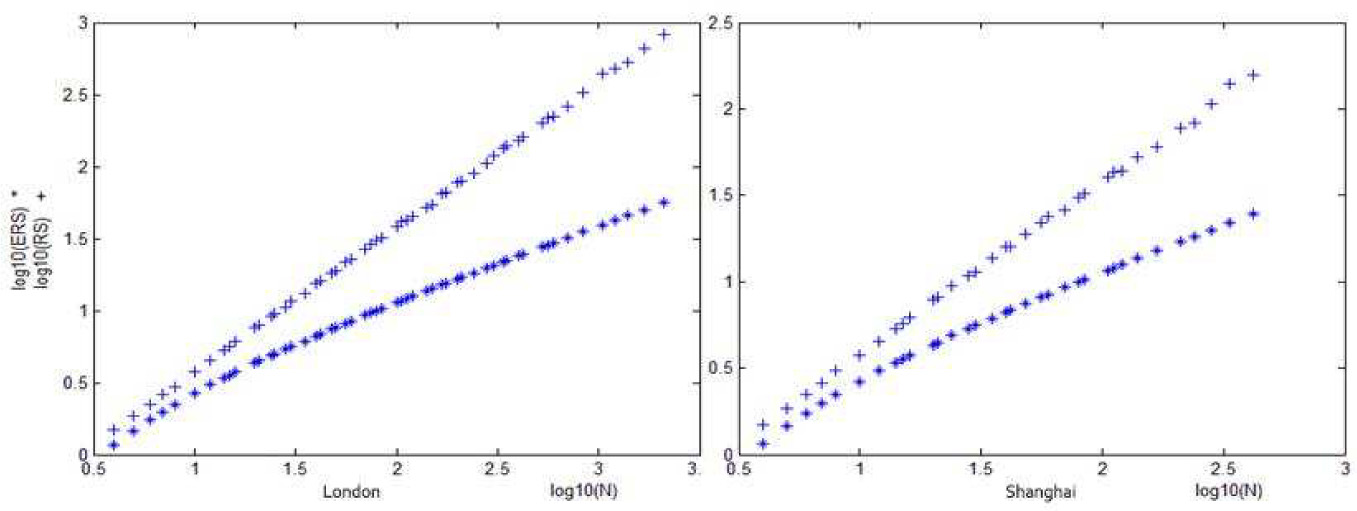
R/S analysis on original gold price data in London and Shanghai

Table 9

Hurst index of gold data under different processing at home and abroad

	Gold in London	Gold in Shanghai
Hurst index of original price series	1.0091	0.9997
Hurst index of residuals of ARMA-GARCH model	0.5921	0.6225
Expectation of Hurst index under i.i.d.	0.5897	0.6301

However, after converting gold price series into logarithmic return series and filtering with ARMA-GARCH model, we obtain a significantly different result (see Figure 2 for details): No difference exists between fitting model residuals of gold price and expectations of i.i.d. series, which means that in the series, long-term memory beyond the ARMA-GARCH process does not exist in series. According to Fig. 2, ln⁡(RnSn) overlaps ln⁡(E(RnSn)) in standardized residuals, and both slope approximates each other, which shows the absense of long-term memory. The result differs from Peters’ due to two reasons. First, Peters employed R/S analysis directly on price series instead of return series. Second, Peters left out the effects of ARMA structure and conditional heteroscedasticity in series. Besides, we can see from the following table that the long-term memory of original price series is quite obvious, while that of return series is relatively weak. In fitting model residuals, long-term memory does not exist.

Figure 2

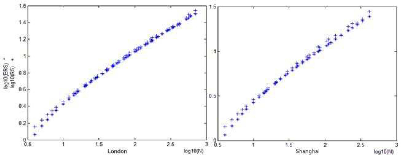
R/S analysis on fitting model residuals of gold return series in London and Shanghai

3.2.2 R/S contrastive analysis of surrogate data

To further verify our assumption (i.e. the absense of deterministic process beyond ARMA-GARCH in series^[10]), we generate a simulated ARMA-GARCH process which shares the same parameters with London gold price process^[11]. Through R/S contrastive analysis and comparison with results of R/S analysis original gold price series in London and Shanghai, we discover from Figure 3 that the linear and nonlinear dependence of gold price series in London and Shanghai can be perfectly described by corresponding ARMA-GARCH model. There is little difference between original series and simulated series, suggesting that ARMA-GARCH process can discribe effectively the characteristics of series.

Figure 3

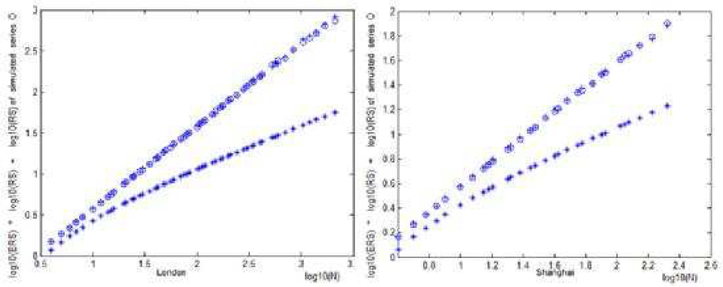
A comparison of R/S analysis on gold original price series in London and Shanghai

Through R/S test on gold price series, we find the long-term memory existing in original price series rather than in residual series filtered with ARMA-GARCH models. Besides, by simply simulating series with ARMA-GARCH model (same parameters with original series), we can obtain identical characteristics in R/S analysis. This further illustrates that the nonlinear characteristics can be effectively discribed with ARMA-GARCH model, and long-term memory beyond ARMA-GARCH model does not exist in gold price series. The nonlinear characteristic of gold price series is conditional heteroscedasticity, instead of chaos.

4.1 Reconstructing phase space with C-C algorithm

To reconstruct phase space, we need two parameters: delay time T_d and embedding dimension m. Chinese scholar Lü[9] discovered that, the result of Lyapunov exponent calculation is sensitive to the choice of parameters in reconstruction of phase space. Current methods to choose reconstruction parameters are: methods of autocorrelation, multiple autocorrelation, mutual information and C-C algorithm. To begin with, since the series to be calculated in the paper are residuals of ARMA-GARCH models which have no obvious autocorrelation characteristic, and no smooth and meaningful autocorrelation or multiple autocorrelation curves can be generated, as a result methods of autocorrelation and multiple autocorrelation cannot be used in this paper. Besides, due to the large data volumn in this paper^[12], the mutual information method which requires high computation cannot be realized in short period of time.

In an overall consideration of mutual information method’s power and computation speed, we choose C-C algorithm in this paper. The idea of C-C algorithm, as well as BDS tests, is based on correlation integral using the following relationship

where r stands for correlation radius (same meaning with the proximity parameters in BDS tests). Brock et al. assumed that, given an i.i.d. series, for any m and r, C(m, N, r, t) approximately equals to C^m(1, N, r, t) at all time, which can be regarded as a measure of nonlinear dependence. Based on this assumption, we could search for delay time T_d by using the figure of S(m, N, r, t) varying with time under nonlinear dependence. The figure can also be viewed as the meaning of changes in autocorrelation function with time under linear dependence.

In order to analyze the nonlinear dependence of series and eliminate short-term spurious correlation, we divide series into t nonintersecting series by time interval t, calculate S(m,Nt,r,t) of each series and obtain the mean. On condition of t = 1, the divided series is the original series itself

Whent = 2, {X_i} is divided into {X₁, X₃, ···, X_N–1} and {X₂, X₄, · · ·, X_N}

For general t, the series is divided into t nonintersecting series, having

Suppose that the time series subjects to i.i.d., for a given m and r, when N approximates infinite, for all r we have

Although actual series might be quite long, it cannot be treated as infinite, and thus S(m, N, r, t) generally does not equal to zero. As a result, the local largest time interval can be chosen as either null point of S¯(m,N,r,t)or the smallest range time point which is least sensitive to radius change, because the space consists of these points is homogeneous. For convenience, we difine range as follows:

4.2 The calculation of Lyapunov exponent

The major calculation methods of Lyapunov exponent are: defination, Wolf method, Jacobian method, P-norm method and Rosenstein method. To employ defination method we need original differential equations that generate dynamic system, which, unfortunately, we cannot obtain. Wolf method is suitable for small sample and low noise time series, which cannot be adopted in this paper because the sample data (daily trading data over 30 years) are large and noisy. Jacobian method, suitable for large and noisy sample, seems adoptable here, but we find that in this method, Lyapunov exponent is calculated using the speed tangent vector evloves with time, and the tangent vector in reconstructed phase space, which consists of ARMA-GARCH model residuals, shakes violently. As a result, the employment of Jacobian method becomes quite difficult.

In the study of chaos, we can determine a system’s chaotic characteristics simply by calculating the largest Lyapunov exponent. Based on that consideration, we choose the Rosenstein method (also called small data set arithmetic), which only calculates the largest Lyapunov exponent. However, traditional Rosenstein method determines delay time T_d by autocorrelation method, while here we use C-C algorithm instead. Besides, to employ Rosenstein method we need to determine the average period^[13]. Here we choose Fast Foourier Transform.

4.3 Lyapunov exponents of gold price abroad

In this paper we use Rosenstein method to calculate largest Lyapunov exponent based on phase space reconstruction by C-C algorithm. Although C-C algorithm can reduce both the time spent in iterative operation and the space complexity, to determine the real minimal value of ρ_S, the total length of series has to be as large as possible. For price series in London and New York, we make use of all 9000 samples from ARMA-GARCH model residuals, while for those in Shanghai, the data amount is too limited to search for smallest value of ρ_S, thus we fail to determine the embedding dimension and reconstruct the phase space. As a result, in this chapter we only listed empirical results of gold data in London and New York.

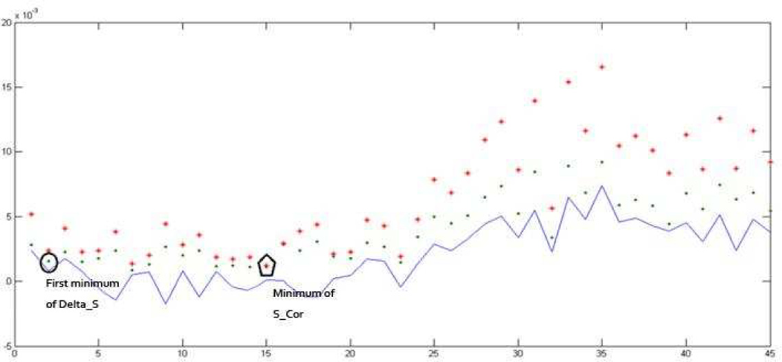
First we determine the parameters in phase space reconstruction-delay time T_d and embedding dimension m (see results Figure 3 and Figure 5). Fig. 4 shows that ∆S reaches the first minimal value when T = 2. We choose T_d = 2 as the actual delay for model residual series of London spot. ρ_S reaches its minimal value when t = 10, i.e. T_w = (m – 1)T_d = 10, from which we obtain embedding dimension m = 6.

Figure 4

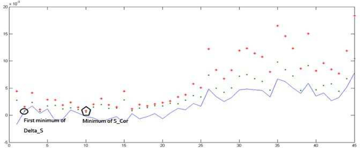
Delay time T_d and embedding dimension m for model residuals of London spot

Figure 5

Delay time T_d and embedding dimension m for model residuals of New York futures

According to Figure 5, ∆S reaches its first minimal value at T = 2. As a result, we choose T_d = 2 as actual delay for gold residual series. The minimum of ρ_S is reached at t = 15, i.e. T_w = (m – 1)T_d = 15 from which we obtain embedding dimension m = 8.

In this paper we determine the average period with Fast Foourier Transform (FFT), which is a fast algorithm to calculate discrete Foourier Transform. Using this algorithm, the multiplication number required by calculation reduce significantly. The larger the transformed sampling point number N is, the more it saves on calculation cost. By FFT calculation, the average period of fitting model residual series in London and New York is 20.0893 and 34.8231.

Finally, we reconstruct phase space using C-C algorithm, and obtained Lyapunov exponents figure of ARMA-GARCH model residuals with revised Rosenstein method. In Figure 6 (upper one), the slope of line stands for the largest Lyapunov exponents of fitting model residuals in New York. As is obvious, although the slope is negative, it approximates zero (–5.113574144831425E–04). This illustrates that fitting model residuals of New York gold futures are random rather than chaotic. According to Figure 6 (lower one) the slope of line is the largest Lyapunov exponent of fitting model residuals in London. From the figure we can clearly see that the slope of the curve approximates zero (0.0062). This illustrates that fitting model residuals of London gold spots are random instead of chaotic.

Figure 6

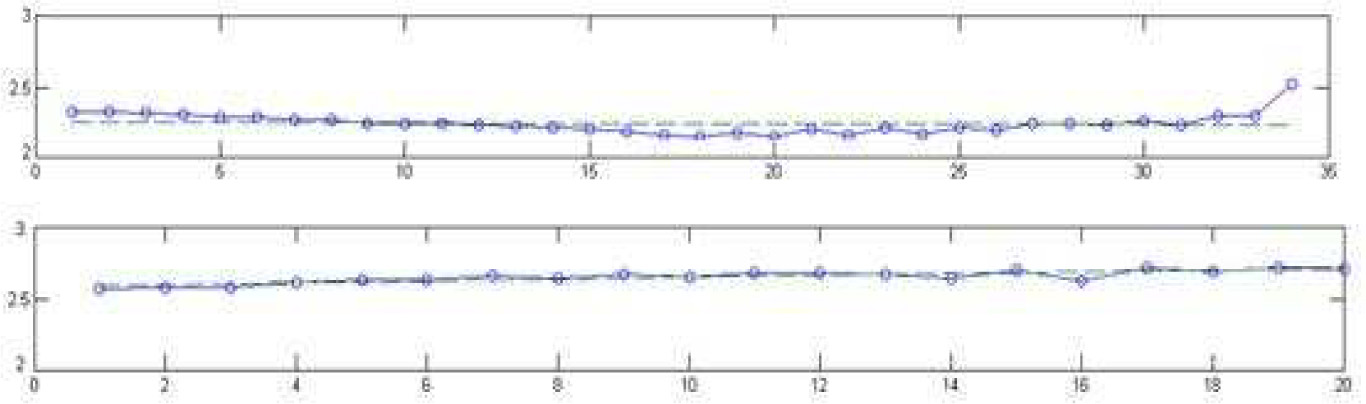
Largest Lyapunov exponents of model residuals in New York (upper) & London (lower)

References

[1] Barnett W A, Gallant A R, Hinich M J, et al. A single-blind controlled competition among tests for nonlinearity and chaos. Journal of Econometrics, 1997, 82(1): 157–19210.1108/S0573-8555(2004)0000261033Suche in Google Scholar
[2] Brock W A, Scheinkman J A, Dechert W D, et al. A test for independence based on the correlation dimension. Econometric Reviews, 1996, 15(3): 197–23510.1080/07474939608800353Suche in Google Scholar
[3] DeCoster G P, Labys W C, Mitchell D W. Evidence of chaos in commodity futures prices. Journal of Futures Markets, 1992, 12(3): 291–30510.1002/fut.3990120305Suche in Google Scholar
[4] Frank M, Stengos T. Measuring the strangeness of gold and silver rates of return. Review of Economic Studies, 1989, 56(4): 553–56710.2307/2297500Suche in Google Scholar
[5] Grassberger P, Procaccia I. Measuring the strangeness of strange attractors. Physica D: Nonlinear Phenomena, 1983, 9(1): 189–20810.1007/978-0-387-21830-4_12Suche in Google Scholar
[6] Kanzler L. Very fast and correctly sized estimation of the BDS statistic. Christ Church and Department of Economics, University of Oxford, 199910.2139/ssrn.151669Suche in Google Scholar
[7] Kim H S, Eykholt R, Salasc J D. Nonlinear dynamics, delay times, and embedding windows. Physica D: Nonlinear Phenomena, 1999, 127(1): 48–6010.1016/S0167-2789(98)00240-1Suche in Google Scholar
[8] Kčcenda E, Briatka L’. Optimal range for the iid test based on integration across the correlation integral. Econometric Reviews, 2005, 24(3): 265–29610.1080/07474930500243001Suche in Google Scholar
[9] Lü J H, Lu J A, Chen S H. Chaotic time series analysis and application. Wuhan University Press, 2002Suche in Google Scholar
[10] Peters E E. Fractal market analysis: Applying chaos theory to investment and economics. John Wiley and Sons, New York, 1994Suche in Google Scholar
[11] Peters E E. Chaos and order in the capital markets: A new view of cycles, prices, and market volatility. John Wiley and Sons, New York, Second edition, 1996Suche in Google Scholar
[12] Rosenstein M T, Collins J J, De Luca C J. A practical method for calculating largest Lyapunov exponents from small data sets. Physica D: Nonlinear Phenomena, 1992, 65(1): 117–13410.1016/0167-2789(93)90009-PSuche in Google Scholar
[13] Wang W N, Wang B H, Chen X. The statistic analysis of the index of Shanghai securities. Operations Research and Management Science, 2003, 12(4): 85–90Suche in Google Scholar
[14] Xie C, Yang N, Sun B. Empirical research on the chaotic dynamical features of exchange rate time series. Systems Engineering — Theory & Practice, 2008, 2008(8): 118–122Suche in Google Scholar
[15] Yang S R, Brorsen B W. Nonlinear dynamics of daily futures prices: Conditional heteroskedasticity or chaos? The Journal of Futures Markets, 1993, 13(2): 175–19110.1002/fut.3990130205Suche in Google Scholar
© 2014 Walter de Gruyter GmbH, Berlin/Boston
Artikel in diesem Heft
- Spatial Dynamics, Vocational Education and Chinese Economic Growth
- The Differential Algorithm for American Put Option with Transaction Costs under CEV Model