Reliability Analysis of Multi-State Engine Units Utilizing Time-Domain Response Data
-
Yongfeng FANG
 ,
Wenliang TAO
,
Wenliang TAO

Abstract
A novel reliability-based approach has been developed for multi-state engine systems. Firstly, the output power of the engine is discretized and modeled as a discrete-state continuous-time Markov random process. Secondly, the multi-state Markov model is established. According to the observed data, the transition intensity is determined. Thirdly, the proposed method is extended to compute the forced outage rate and the expected engine capacity deficiency based on time response. The proposed method can therefore be used for forecasting and monitoring the reliability of the multi-state engine utilizing time-domain response data. It is illustrated that the proposed method is practicable, feasible and gives reasonable prediction which conforms to the engineering practice.
1 Introduction
One inherent weakness of classical reliability theory is that the system and the units are always described just as functioning or failed[1]. At any time, the system is in one of these two states. In the real world, many systems can perform their tasks at several different levels. A system that can have different task performance levels is named multi-state system (MSS)[2,3]. MSS reliability has received a substantial amount of attention in the past four decades and has been widely used and proven to be very beneficial to several industries such as power systems, engines, electronic products, etc[4,5].
The MSS was introduced in the 1970's[6,7]. In these works, the basic concepts of MSS reliability were formulated. Much work in the field of reliability analysis was devoted to the binary-state systems, where only the complete failures are considered[8,9]. Although multi-state reliability models provide more realistic and more precise representations of engineering systems, they are much more complex and present major difficulties in system definition and performance evaluation. Currently, the multi-state reliability assessment instead of a two-state system assessment for the engine has been proposed[10-12]. However, the proposed methods for multi-state engine reliability assessment are not accurate especially when the engine unit reliability has marginal situation.
In recent years, the research study of Markov chain and semi-Markov chain has been increasing. The theory is gradually developed and its application in the reliability of the system has been explored[13-15]. System reliability, availability, average operating time can be predicted by using the Markov chains and semi-Markov Chain. The reliability of coal-fired generating units was studied by using a single Markov model[16,17]. The reliability problems of various engineering systems with discrete-state and continuous-time were presented and the problems were solved by using Markov model with discrete and continuous time[18-22]. However, there is limited literature on multi-state engine system reliability studied by using the Markov chains and semi-Markov chain. The reliability of multi-state generator has been studied by using discrete-state and continuous-time Markov model and the predicted results can be used for short-term forecasting of this type of equipment[23].
On the basis of these articles, the multi-state random process of engine system has been studied by using discrete-state and continuous-time Markov model and semi-Markov model based on the actual failure of engine system. The appropriate multi-state Markov model has been established and the multi-state engine reliability based on time response can be assessed by using the proposed model. It is illustrated that the proposed method is practicable, feasible and gives reasonable prediction which conforms to the engineering practice.
2 The Multi-State Markov Model
At any time t during the work period T of an engine unit, the work capacity of the engine can be indicated by using real interval [0,g], where g is the maximum work capacity of the engine at time t. Clearly, this is continuous-state random process. However, the process can be substituted using discrete-state continuous-time process G(t) which is elaborated as follows.
The two special states of the engine are denoted by 1 and N which correspond to g1 = 0 that the engine has completely failed and gN = g that the engine produces output energy at a normal level, respectively.
The interval [0,g] can be divided into N - 2 subintervals and the length of each subinterval is
If G(t) − ((i - 1)Δ g,(i - 1)Δ g],i = 2, ⋯ ,N - 1, the state of the random process G(t) is denoted by i(i = 2,3,⋯N−1) at time t and its work energy is denoted by gi.
The work energy gi of the random process G(t) in state i is the average energy of ((i − 1) Δ g, (i − 1) Δ g].
The original continuous-state random process G(t) is converted to discrete-state continuous-time random process GD (t) through quantitative techniques. The random process GD (t) has N(N = 1,2,⋯,N) different output energy levels gi . The random process GD (t) can be described by using Markov stochastic process with its transition states. The transition of N states to each other is illustrated in Figure 1. The transition from state i to state j is denoted by ai,j whereas the transition from state N - 1 to state N - 2 is denoted by aN - 1,N - 2 and so on. Each state i corresponds to engine work energy gi . The m-th sojourn time in state i of the unit is denoted by
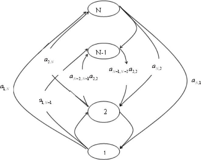
Multi-state Markov model for engine unit
3 Determination of Transition Intensity
GD (t) is a discrete-state continuous-time Markov process, if the transition time of the unit from state i to state j(i ≠ j) can be neglected, only the instantaneous moment of the transition is interested, thus GD (t) can be considered as a discrete-state and discrete-time random process which is denoted by GDi(n),n = 0,1,⋯. This is an embedded Markov process and this process can be entirely determined by using its initial state probability distribution and probability of one step transition which is denoted by πij, i, j = 1, 2, ⋯ , N.
The cumulative probability distribution function of the unit transition from state i to state j(i ≠ j) is shown as follows.
The first transition probability of the unit from state i to state j at time t is denoted by Qij(t), i, j = 1,2, ⋯, N. The nuclear matrix Q(t) of the random process GD (t) consists of all Qij (t) and can be calculated as follows.
Based on Equation (1), Equation (2) can be rewritten as follows.
The cumulative probability distribution function of sojourn time Ti of the unit in state i is written as follows.
It is shown from Equation (4) that Ti is considered to obey the exponential distribution and the mean of Fi (t) can be calculated as follows.
where
On the other hand, the mean obtained by using observed samples is given as follows.
The total intensity of the transition from any states can be estimated by using Equation (7) which can be obtained by using Equations (5) and (6).
The probability of one step transition can be obtained by using embedded Markov random processing.
Equation (8) can then be further simplified by using Equation (4) as follows.
The single transition intensity in state i can be obtained by rearranging Equation (4) as follows.
The single step transition probability of embedded Markov chain can be computed by using unit work energy.
Finally, the transition intensity can be computed by using Equations (7), (10) and (11).
For the multi-state Markov system with N states, the transition intensity can be written as follows.
where
In summary, the algorithm for determination of transition intensity for multi-state Markov system with N states is given as follows.
Step 1 The system will be quantitatively processed by using the method described above. Every state i of the engine will be corresponded to the output work energy gi.
Step 2 The summation of sojourn time of the unit in every state i can be computed by using the observed data.
Step 3 The transition intensity from state i to state j is computed by using Equations (16) and (17).
4 Worked Examples
4.1 Computation of Transition Intensity
A fuel engine is used as an example to verify the proposed multi-state Markov model. The normal output power of the fuel engine is 288KW and its service period is limited to T = 5 years. The multi-state Markov model can be established by using the above algorithm. The two special states of the engine correspond to g1 = 0KW that the engine has completely failed and g4 = 288KW that the engine produces output energy at a normal level. The interval [0, 288] can be divided into 2 subintervals and the length of each subinterval is
Thus, the two intervals are given as [0,144]KW and [144,288]KW. The other two output energy levels are computed as g2 = 123KW and g3 = 241KW by using the result that was observed in the last five years. The transition intensity
The number of transition from state i to state j and the sojourn time in state i of the unit is shown in Table 1.
The number of transition and the accumulated time
| State | 1 | 2 | 3 | 4 | output energy (KW) | accumulated time |
|---|---|---|---|---|---|---|
| 1 | 0 | 6 | 1 | 0 | 0 | 75 |
| 2 | 1 | 0 | 11 | 1 | 123 | 34 |
| 3 | 0 | 3 | 0 | 37 | 241 | 104 |
| 4 | 6 | 4 | 28 | 0 | 288 | 40711 |
4.2 Analysis of Four-State Model of Engine Unit
The transition of four-state Markov model is shown in Figure 2. The steady-state probabilities of the states 1, 2, 3 and 4 are given as follows, respectively.

Four-state (MSS) Markov model for engine unit
The probabilities Pi (t), (i = 1,2,3,4) of the state i can be obtained by solving the following differential equations (21) at any time under specific initial conditions.
Once the probabilities of the states have been obtained, the stability probability of the engine in state i can be calculated using Equation (22).
4.3 Reliability Prediction Based on Time Response
In electrical engineering, forced outage rate (FOR) of engine is an important evaluation indicator. FOR is the probability that the engine will not be available for service when required and the output energy of the engine is 0. It is a function of time which stops in state 1 as follows.
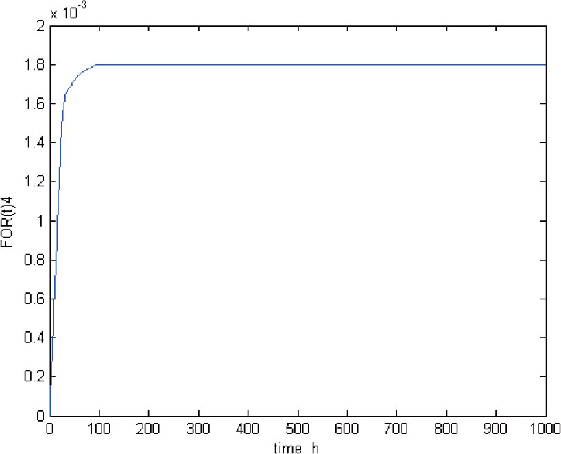
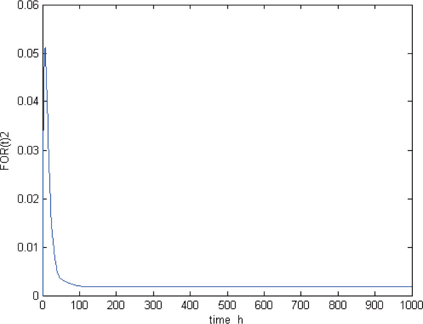
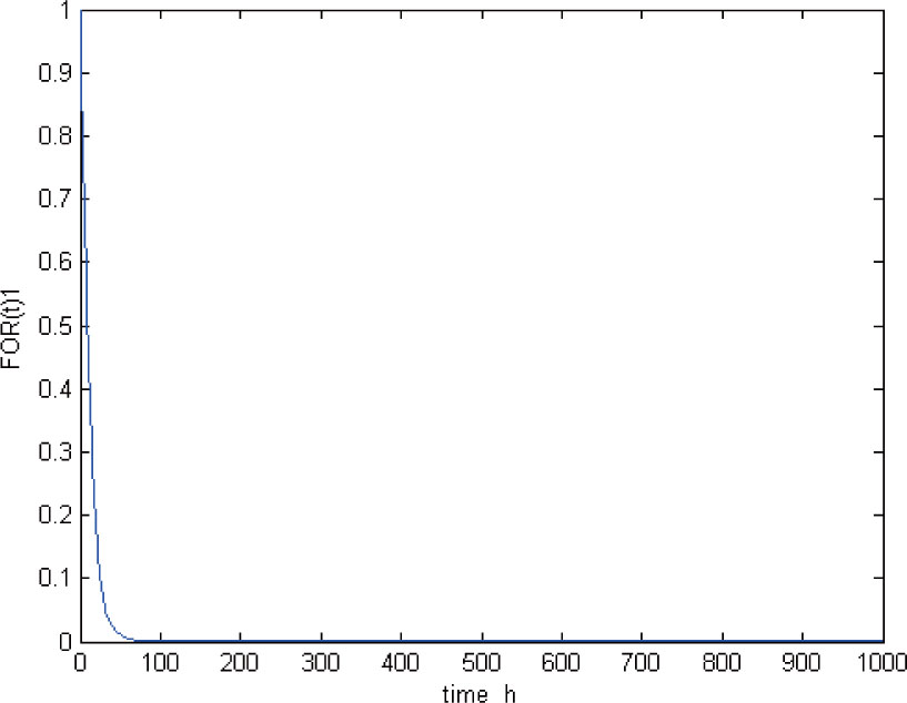
FOR(t) is computed based on initial conditions of the differential Equation (21). Four cases of initial conditions are studied and are preset as follows.
The calculated FOR(t) for Cases 1, 2, 3 and 4 are shown in Figures 3, 4, 5 and 6, respectively. It is shown that the engine is stable after 80 hours and the stability probability in state 1 at that time is estimated as follows.
FOR(t) under initial condition (24) for Case 1

FOR(t) under initial condition (25) for Case 2
FOR(t) under initial condition (26) for Case 3
FOR(t) under initial condition (27) for Case 4
Based on Equation (28), FOR of the engine is stabilized with the probability of 0.0018 under the initial conditions of (24), (25), (26) and (27). It is also noticed that the maximum FOR under the initial conditions of (25), (26) and (27) is larger than that under the initial condition of (24). The reason is that if state i is closer to state 1 than state j when the unit is transited from state i to state j, the engine has a higher probability of malfunction. Obviously, the engine is turned into fault state when it is operated under the initial condition of (27) which can be validated by the real situation.
If the engine can be supplied to output capacity of W = 200KW at the 1000th hour, it will be transited to state 2 and the output energy can not be reached to 123KW. In other words, the following capacity deficiency (CD) will be produced.
If it will be transited to state 1, the output energy can not be reached to the requirement. In other words, the following capacity deficiency (CD) will be produced.
The expected capacity deficiency (ECD) is a function of time response and can be obtained as follows.

ECD(t) under initial condition (24) for Case 1
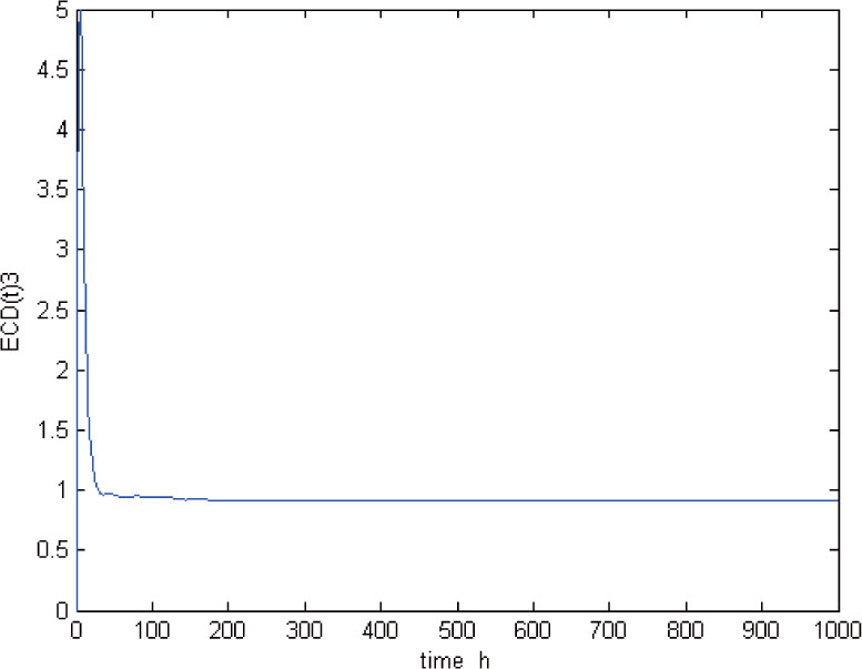
ECD(t) under initial condition (25) for Case 2

ECD(t) under initial condition (26) for Case 3

ECD(t) under initial condition (27) for Case 4
The calculated ECD for Cases 1, 2, 3 and 4 under the initial conditions of (24), (25), (26) and (27) are shown in Figures 7, 8, 9 and 10. It is shown that the variation regular of the CD is the same as the variation regular of the FOR. Based on ECD(t)i, the expected energy not supplied (EENS) at any time can be computed using Equation (32) as follows.
5 Conclusions
The output power of engine system is discretized and modeled as a discrete-state continuous-time Markov random process. The multi-state Markov model is then established. According to the observed data, the transition intensity is determined. The proposed method is then extended to compute the forced outage rate and the expected engine capacity deficiency with respect to time. The proposed method can be used for forecasting and monitoring the reliability of the multi-state engine utilizing time-domain response data. It is illustrated that the proposed method is practicable, feasible and gives reasonable prediction which conforms to the engineering practice.
References
[1] Fang Y, Chen J, Tee K F. Analysis of structural dynamic reliability based on the probability density evolution method. Structural Engineering and Mechanics, 2013, 45(2): 201-209.10.12989/sem.2013.45.2.201Suche in Google Scholar
[2] Natvig B. Multi-state systems reliability theory with application. New York: John Wiley & Sons, 2011.10.1002/9780470977088Suche in Google Scholar
[3] Lisnianski A, Levitin G. Multi-state system reliability: Assessment, optimization, applications. World Scientific Press, 2003.10.1142/5221Suche in Google Scholar
[4] Billinton R, Allan R N. Reliability evaluation of power systems. New York: Plenum Press, 1996.10.1007/978-1-4899-1860-4Suche in Google Scholar
[5] Manoukas G E, Athanatopoulou A M, Avramidis I E. Multimode pushover analysis based on energy equivalent SDOF systems. Structural Engineering and Mechanics, 2014, 51(4): 531-546.10.12989/sem.2014.51.4.531Suche in Google Scholar
[6] Barlow R E, Wu A S. Coherent system with multi-state components. Mathematics of Operations Research, 1978, 3(1): 275-281.10.1287/moor.3.4.275Suche in Google Scholar
[7] Ross S. Multi-valued state component systems. The Annals of Probability, 1979, 7(2): 379-383.10.1214/aop/1176995096Suche in Google Scholar
[8] Fang Y, Wen L, Tee K F. Reliability analysis of repairable k-out-n system from time response under several times stochastic shocks. Smart Structures and Systems, 2014, 14(4): 559-567.10.12989/sss.2014.14.4.559Suche in Google Scholar
[9] Tee K F, Khan L R. Reliability analysis of underground pipelines with correlation between failure modes and random variables. Journal of Risk and Reliability, Proceedings of the Institution of Mechanical Engineers, Part O, 2014, 228(4): 362-370.10.1177/1748006X13520145Suche in Google Scholar
[10] Billinton R, Gao Y, Huang D, et al. Adequacy assessment of wind-integrated composite generation and transmission systems. Innovations in Power Systems Reliability, Springer Series in Reliability Engineering, London: Springer, 2011.10.1007/978-0-85729-088-5_4Suche in Google Scholar
[11] Reshid M, Abd Majid M. A multi-state reliability model for gas fueled cogenerated power plant. Journal of Applied Science, 2011, 11(11): 1945-1951.10.3923/jas.2011.1945.1951Suche in Google Scholar
[12] Vosooq A K, Zahrai S M. Study of an innovative two-stage control system: Chevron knee bracing & shear panel in series connection. Structural Engineering and Mechanics, 2013, 47(6): 881-898.10.12989/sem.2013.47.6.881Suche in Google Scholar
[13] Aven T. On performance measures for multi-state monotone systems. Reliability Engineering and System Safety, 1993, 41(3): 259-266.10.1016/0951-8320(93)90078-DSuche in Google Scholar
[14] Brunelle R D, Kapur K C. Review and classification of reliability measures for multi-state and continuum models. Transactions of Institute of Industrial Engineers, 1999, 31(2): 1171-1181.Suche in Google Scholar
[15] Limnios N, Oprian G. Semi-Markov processes and reliability in statistics for industry and technology. Boston: Birkhauser, 2001.10.1007/978-1-4612-0161-8Suche in Google Scholar
[16] Goldner S. Markov model for a typical 360 MW coal fired generation unit. Communication in Dependability and Quality Management, 2006, 9(1): 9-24.Suche in Google Scholar
[17] Jahanshahia M R, Rahgozar R. Free vibration analysis of combined system with variable cross section in tall buildings. Structural Engineering and Mechanics, 2012, 42(5): 715-728.10.12989/sem.2012.42.5.715Suche in Google Scholar
[18] Barbu V, Boussemart M, Limnios N. Discrete time semi-Markov processes for reliability and survival analysis. Communications in Statistic, Theory and Methods, 2004, 33(11): 2833-2868.10.1081/STA-200037923Suche in Google Scholar
[19] Koroliuk V S, Limnios N, Samoilenko I. Poisson approximation of impulsive recurrent process with semi-Markov switching. J. Stochastic Analysis and Applications, 2011, 29(5): 769-778.10.1080/07362994.2011.598780Suche in Google Scholar
[20] Menshikova M, Petritis D. Explosion, implosion, and moments of passage times for continuous-time Markov chains: A semimartingale approach. Stochastic Processes and Their Applications, 2014, 124(7): 2388-2414.10.1016/j.spa.2014.03.001Suche in Google Scholar
[21] Barbu V, Limnios N. Semi-Markov chain and hidden semi-Markov models toward applications in lecture notes in statistic. Berlin: Springer, 2008.Suche in Google Scholar
[22] Janssen J, Manca R. Semi-Markov risk models for finance, insurance and reliability. Berlin, Germany: Springer-Verlag, 2007.Suche in Google Scholar
[23] Lisnianski A, Elmakias D, Laredo D, et al. A multi-state Markov model for a short-term reliability analysis of a power generating unit. Reliability Engineering and System Safety, 2012, 98(3): 1-6.10.1016/j.ress.2011.10.008Suche in Google Scholar
© 2016 Walter de Gruyter GmbH, Berlin/Boston
Artikel in diesem Heft
- Retrospective and Prospective Analysis on the Trends of China’s Steel Production
- The Coordination and Optimization of Closed-Loop Supply Chain with Lots of Factors
- The Effect of Visual Merchandising, Sensational Seeking and Collectivism on Impulsive Buying Behavior
- Quantiles on Stream: An Application to Monte Carlo Simulation
- Empirical Analysis of AH-Shares
- Reliability Analysis of Multi-State Engine Units Utilizing Time-Domain Response Data
- A Quantitative Method for Selection of Enterprise Cloud Computing Models
- The Command Decision Method of Multiple UUV Cooperative Task Assignment Based on Contract Net Protocol