Graphene in curved Snyder space

1 Introduction

Recently, an increasing interest is dedicated to the study of classical and quantum mechanics on a quantized space-time [1], [2], [3], [4], [5], [6], [7], [8], [9], [10]. Historically Hartland S. Snyder was the pioneer of this idea. In 1947, he proposed a fundamental length and stated noncommutative operators of the quantized space-time coordinates with four translation generators of the algebra [11]. Originally, this attempt was solely aimed to solve the problems connected to ultraviolet (UV) divergences in quantum field theory. In the same year, he published a second article in which he discussed the effect of quantized space-time on the electromagnetic field theory [12]. However, this article was his last published article on this subject. Meanwhile, due to the development of renormalization techniques, the UV divergences problem in quantum field theory has resolved. For this reason, Snyder’s idea was not used more than some articles [13], [14], [15], [16], [17], [18]. The curved space selected by Snyder is the (3+1) de Sitter space, fabricated as the homogeneous space:

where SO (4, 1) is the group of isometriesf, H = SO (3, 1) is the Lorentz group while the Snyder-Galilean models are achieved as the nonrelativistic limit of the Snyder–Lorentzian models. The relativistic modified quantum algebra proposed by Snyder is based on the following commutation relations:

Here, η_μν is the metric tensor where its signature is[η_μν] = diag(−1111). β is a coupling constant proportional to the Planck length, J_μν are the generators of Lorentz transformations, while μ and ν are the space-time indices with μ, ν = 0, 1, 2, 3. Via the presence of a fundamental constant, β, the model is seen to be an example of doubly (or deformed) special relativity [19]. Depending on the positive or negative values of the beta parameter, the model is called as Snyder and anti-Snyder model, respectively [2].

In 1947, in order to make Snyder’s theory invariant under the group of translations that are based on the conformal group SO (1, 5), Yang extended Snyder’s model to a de Sitter space-time background [13]. The resulting model is characterized by three invariant scales, the speed of light in vacuum, c, the Snyder parameter β, and the cosmological constant Λ. Therefore sometimes, that model is preferred to be named as triply special relativity instead of the Snyder-de Sitter (SdS) model. In momentum space a one-to-one correspondence between the Snyder/anti-Snyder model and the de Sitter/anti-de Sitter space-time is reported in a study by Guo et al. [20].

The SdS model’s algebra is constructed with the position X_μ, momentum P_μ and Lorentz generator J_μν operators, which obey the following algebra [21], [22].

This algebra can be regarded as a nonlinear realization of Yang model. It should be noted that α and β are the coupling constants with dimension of inverse length and inverse mass, they are defined as the square root of the cosmological constant α∼10−24cm−1 and with mass of Planck β∼105g−1 [19]. In the limits α → 0, and β → 0 the algebra (3) reduces to the Snyder model in flat space and to the de Sitter algebra, respectively [23], [24]. The SdS phase space can be realized in six-dimensional space as SO (1, 5)/SO (1, 3) × O (2) if α, β > 0 and SO (2, 4)/SO (1, 3) × O (2) if α, β < 0 [5]. Recently, many authors have condensed their studies on the discussions over the deformed canonical commutation relations [5], [25], [26], [27], [28], [29], [30], [31], [32], [33], [34], [35], [36].

In the last decade, Graphene has attracted the attention of theoretical and experimental physicists [37], [38], [39]. A graphene material has a two-dimensional structure that is constituted from carbon atoms in the honeycomb lattice form which yields superior mechanical properties in addition to optical and electronic properties [40], [41], [42], [43]. In the theoretical perspective, a low energy excitation in a single graphene layer is described by the massless Dirac equation [44], [45].

In this paper, we consider massless fermions located in a graphene layer under the effect of a perpendicular external magnetic field. We solve the Dirac equation in the SdS model and obtain the energy eigenvalue function. Then, we explore the thermodynamic functions in order to discuss the effects of the fundamental scales of the SdS model. We present the manuscript as follows: In section 2, we introduce the SdS model briefly. In section 3, we solve the massless Dirac equation. We obtain the energy spectrum function analytically. Next, in section 4 we define the partition function. At the high-temperature limit, first, we derive the internal energy functions, and then, the heat capacity and the entropy functions. We demonstrate the thermodynamic functions versus temperature and discuss the effect of the fundamental coupling constants of the SdS model. We end the manuscript with a brief conclusion.

2 Curved Snyder model

In the nonrelativistic curved Snyder model, the modified commutation relations between the position and momentum operators are given by [22], [36]:

where J_jk = (X_jP_k−X_kP_j). In [22], [36], one set of the X_j and P_j operators which satisfies the algebra is expressed in the canonical coordinates as

Here, λ is an arbitrary real parameter. Note that p_j is bounded in the range of −1β<pj<1β. If we consider a case, where (〈P_j〉 = 〈X_j〉 = 0), we obtain the uncertainty relation as

In one dimension case, Eq. (7) reduces to

As a conclusion, the modification in the algebra produces the following minimal uncertainties in both position and momentum measurements

We note that, if α, β < 0 minimal uncertainties do not emerge and all real values of Piare allowed. Before we proceed through the next section, it is worth remarking the change of the definition of the scalar product with the following form of [22],

3 Graphene in an external magnetic field

In this section, we solve the (2+1)-dimensional massless Dirac equation in the curved Snyder model in the presence of the uniform magnetic field B, which is directed along the z axis. We assume B > 0 and employ A=B2(−X2,X1) gauge. We start with the Dirac equation

Here, ψ is a two-dimensional wave function that describes the electron states between the two Dirac points A and B, while the Dirac Hamiltonian is

where V_F = (1.12 ± 0.02)×10⁶ ms⁻¹ is the Fermi velocity. We define a fundamental length scale, ℓ_B, in the presence of an external magnetic field via ℓB=ℏceB, and express the Hamiltonian in the matrix form

with two Hamiltonian operators for the two Dirac points A and B as

We write the two-component wave function as

where ψ^A and ψ^B are two-dimensional eigenstates. To obtain the energy eigenvalue equation of the wave function at the Dirac point A, we solve the following system of two coupled equations:

Out of the coupled system, we obtain the following decoupled differential equation for the component ψ^A.

Then, we employ the position and momentum operators given in Eqs. (5) and (6). We find

In order to simplify the differential equation we assume

Then, (𝒳jРj+Рj𝒳j) term vanishes and Eq. (20) becomes

where

and

We perform a change of the variable

which maps the allowed range from −1β<p<1β to −π2β<ρ<π2β. Equation (22) reduces to the form of

By ansatz, we assume ΦA=sinμ(βρ)cosδ(βρ)Ϝ. Then, Eq. (26) becomes

We fix the parameter δ by requiring the coefficient of the tan2(βρ) to vanish:

We determine the roots of the quadratic equation of δ as

We note that the second root does not lead to a physically acceptable wave function unless we impose the condition ℓℬ2>1/2. However, this condition is valid only for small enough field strengths. Therefore, we use the first root in Eq. (29). We find the reduced equation in the form of

We define a new variable q=sin2(βρ). Then, Eq. (30) turns into the form of the hypergeometric equation [46].

This equation has a regular solution at q = 0 that is written in terms of hypergeometric functions as

with the following parameters:

The hypergeometric function F(a, b, c; q) is determined by the hypergeometric series [46] as follows:

where the parameters of the hypergeometric series are given by

The series reduces to a polynomial if a or b is a negative integer. Using the expressions of b, we finally obtain

where θ=α+ℏ2β4ℓB4. We would like to emphasize that the latter equation represents the main result of our paper. We observe that the introduced deformed Heisenberg algebra has influence on results. We also note that the energy spectrum depends on n², which is a feature of hard confinement. Furthermore, the energy spectrum values increase proportional to n for the large quantum number n. It should be pointed out that for n = 0, the energy level E_n = 0, which means the energy level at higher levels (n = 1, 2, …) are distributed symmetrically around n = 0. In addition, the energy level is proportional to n2, which implies the energy spacing between adjacent levels is not constant. For large n the energy spacing becomes constant

where ωc=2VFθ can be interpreted as classical cyclotron frequency. As α and β are small in comparison with the other quantities in the theory, we expand (37) to first order in α and β, we obtain

Here, the first term represent the Landau levels of electrons in graphene while the second term is the quantum gravity correction. Now, let us consider the following particular cases.

1. In the limit β → 0, we recover the results for anti-de Sitter space [47].

1. In the limit α → 0, we obtain the energy spectrum in the Snyder space.

1. In anti–Snyder-de Sitter model where α < 0 and β < 0, the energy spectrum is,

in this case the energy spectrum E_n becomes complex when the quantum number n is large. This stipulates an upper bound on the allowed values of n.

1. In the limit β → 0 and α → 0, we get the ordinary quantum mechanical result [48], [49].

1. If δ=1−12ℓℬ2, the energy spectrum is,

On another side, if a or b is a nonnegative integer, the hypergeometric series converges absolutely for all values of |q|<1 [50] and,

For to make the hypergeometric function to be regular at q = 1, we must impose ℓℬ2>1 , which is valid only for small enough field strengths. In the case where the particles cannot be bounded, only scattering solutions occur and the energy spectrum becomes continuous.

In order to demonstrate the influence of the modified algebra on the energy levels, we plot the energy levels ϵ=En,μ=0ℏVF versus the quantum number, n, by employing different values of the deformation parameters in Figure (1). We observe that the contribution of the α parameter is more significant than the β parameter.

Figure 1:

En,μ=0ℏVF versus the quantum number n for different values of the deformation parameters.

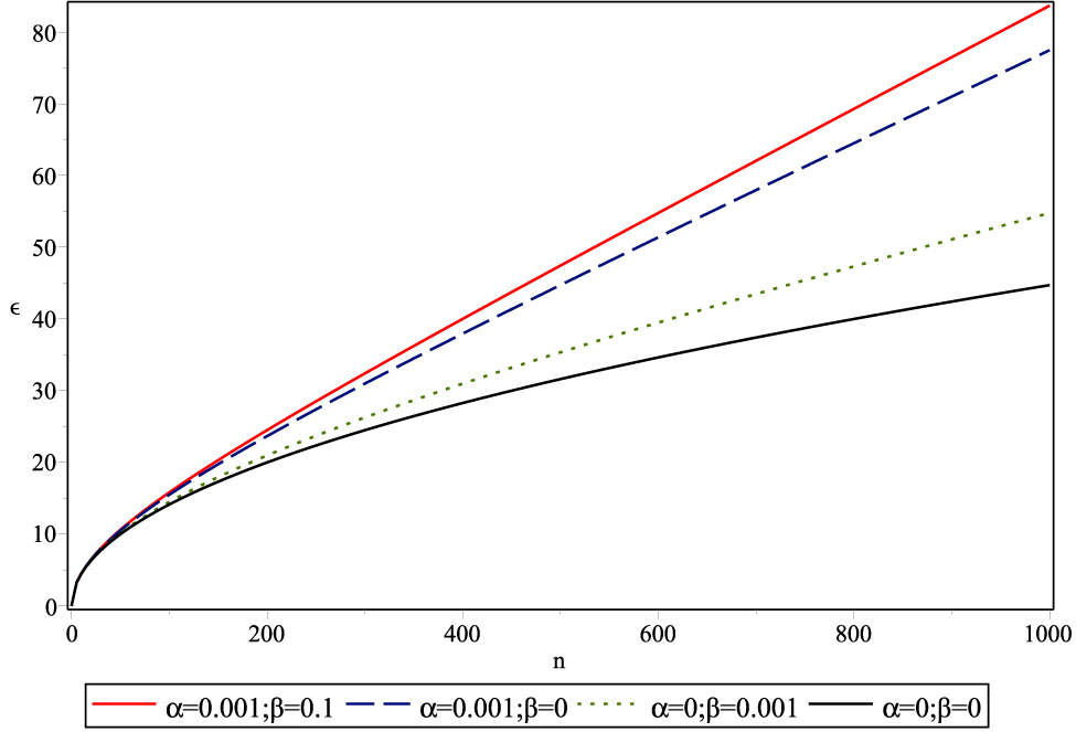
It should be noted that the dependence of the energy levels on SdS parameters is only through θ, and this can be easily quantified. For weak magnetic fields, the parameter θ identified as the cosmological constant, θ∼α∼10⁻⁴⁸. If the magnetic field is extremely strong the parameter θ take the value θ∼e2B2βc2∼10−44B2.

4 Thermodynamic functions

It is a well-known fact that an electron gas obeys the Fermi–Dirac quantum statistic. However, in high temperatures or with the consideration of the electron gas in a low density, the Maxwell–Boltzmann statistic can be used instead [51]. In this section we aim to determine the thermodynamic properties of the of the graphene under a magnetic field in SdS space. We suppose only fermions with positive energy (E ≥ 0) constitute the thermodynamic ensemble. Since we ignore the particle–particle interactions, we take neither negative-energy excited states nor the phenomenon of creation of particles into account [49], [52]. Therefore, we assume the partition function contains only a sum over positive-energy states. We note that this is an enormous simplification characteristic. We begin by computing the partition function of a single particle of the system, Z, for the fixed angular momentum (μ = 0):

Here, K denotes the Boltzmann constant, T represents the thermodynamic temperature and E_n is the energy eigenvalues. We use the derived energy eigenvalue function given in Eq. (39) in Eq. (46). We obtain the partition function in the form of

Since α and β are small in comparison with the other quantities in the theory, we expand Eq. (47) till to the first order of α and β. We obtain

where β¯=1τ, and τ is the reduced temperature defined with

Here, T0=ℏVF2KℓB is the temperature reference value, for instance when B = 18T, the value of this temperature becomes T₀ = 3551 K. It is worth noting that the first term in Eq. (48) is the ordinary partition function of the graphene under a magnetic field

We calculate the second and third terms of Eq. (48) by using the derivatives of Eq. (50) as follows:

After all, we obtain the total partition function of the system in the SdS space in the form of

Next, we derive the thermal properties of our system, such as the internal energy and the specific heat through the numerical partition function Z via the following relations:

We take ℓB=ℏ=c=K=1, and demonstrate all profiles of the thermodynamic quantities as a function of τ for various values of the SdS parameters.

First, we plot the partition function versus τ in Figure (2). We observe a monotonic increase in the partition function in the ordinary quantum mechanic limit. This characteristic behavior drastically changes in the existence of the SdS model parameters. We observe a decrease in the partition function while the temperature increases at the high-temperature values. The amount of the decrease in the partition function value increases when de Sitter space-time is taken into account instead of the Snyder model.

Figure 2:

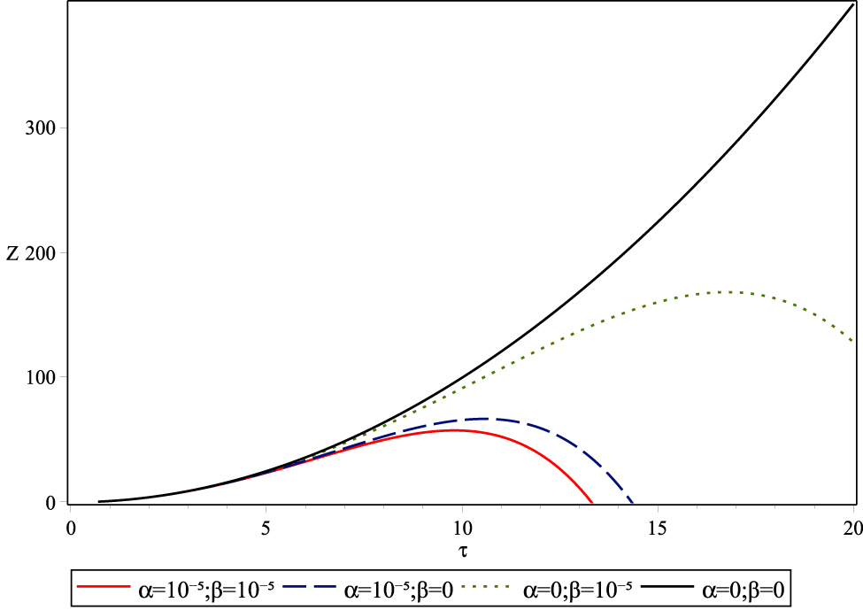
Partition function versus the reduced temperature.

We present the characteristic behavior of the internal energy function versus the dimensionless reduced temperature for different values of the SdS parameters in Figure (3). In the ordinary quantum mechanic limit, we observe a linear increase. When we consider a comparison between the role of the and parameters, we observe that the internal energy is being modified significantly in the de Sitter space, rather than the Snyder model because of the dependence on the strength of the magnetic field. We also see that in the vicinity of zero, there is no difference between the standard and the modified internal energy, which implies that the effects of quantum gravity become more obvious only at high temperatures.

Figure 3:

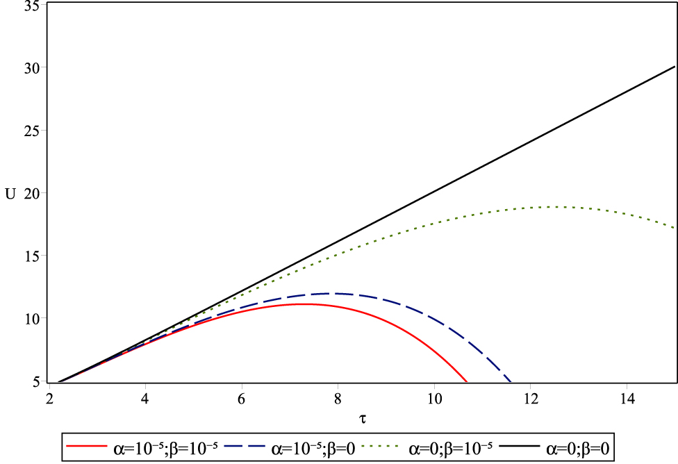
Internal energy versus the reduced temperature.

Finally, we illustrate the heat capacity function versus the reduced temperature in Figure (4) by considering different values of the SdS parameters. In the ordinary quantum mechanic limit, we observe that the heat capacity will tend to a constant value at high temperature. We also see a decrease in the heat capacity function for high-temperature in the existence of (α, β). When we consider a comparison in between the parameters, like the other cases, we realize that the role of the parameter α is more significant than the β parameter.

Figure 4:

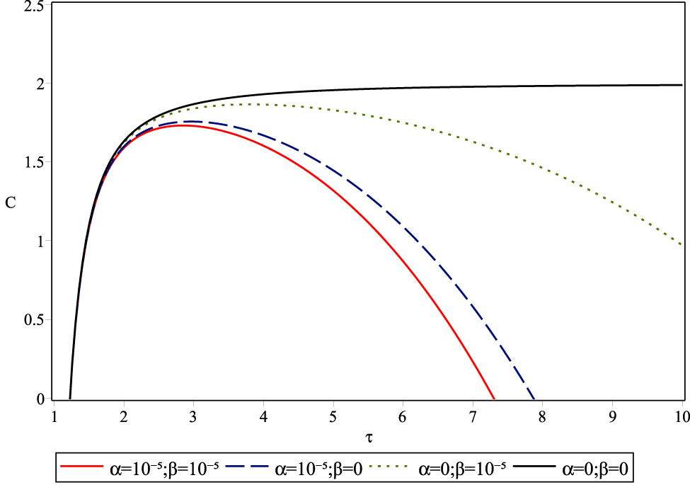
Specific heat function versus the reduced temperature.

It is worthwhile to note that all thermodynamic quantities obtained numerically in our work show that the effects of the curved Snyder model on the statistical properties of graphene are important only in the high-temperature regime, contrary the case at low temperatures. The effect of the SdS model becomes insignificant and the curves join rapidly as the temperature decreases. Our conclusion that the quantum gravity effects have concrete effects specifically at high-temperature limits.

Finally, when SdS parameters α = β = 0 our results agrees exactly with that of [48]. One of the biggest issues in physics at present is to combine the quantum theory and the theory of general relativity into a unified framework, different approaches toward such a theory of quantum gravity have been elaborated. Despite that, one major obstacle is the absence of experimental confirmation of quantum gravitational effects [53]. The results we presented here may afford a source of information to probing Planck-scale physics in future experiments.

5 Conclusion

In this paper, we considered a graphene layer which is under the influence of an external magnetic field. We assumed the applied field to be perpendicular to the layer and solved the massless Dirac equation in the (2+1) dimension in the SdS model. We derived an analytic solution to the wave and energy eigenvalue functions. The essential characteristic of energy levels is the existence of zero-energy states.

Then, we investigated some of the statistical characteristics of the considered system at high temperatures by comparison of the thermodynamic functions. We found that the fundamental scales of the model have an important role on the thermal quantities. We comprehended that the contribution of the deformation parameter of the de Sitter space-time is more significant than the Snyder model parameter. We also found the influence of SdS model can be seen only at high-temperatures limits.

References

[1] S. Mignemi, “Classical and quantum mechanics of the nonrelativistic Snyder model,” Phys. Rev. D, vol. 84, no. 2, p. 025021, 2011, https://doi.org/10.1103/physrevd.84.025021.Search in Google Scholar
[2] S. Mignemi, “Classical and quantum mechanics in the Snyder space,” J. Phys. Conf., vol. 343, no. 1, p. 012074, 2012, https://doi.org/10.1088/1742-6596/343/1/012074.Search in Google Scholar
[3] S. A. Franchino-Vinas and S. Mignemi, “Worldline formalism in Snyder spaces,” Phys. Rev. D, vol. 98, no. 6, p. 065010, 2018, https://doi.org/10.1103/physrevd.98.065010.Search in Google Scholar
[4] S. Meljanac, S. Mignemi, J. Trampetic, and J. You, “Nonassociative Snyder ϕ4 quantum field theory,” Phys. Rev. D, vol. 96, no. 4, p. 045021, 2017, https://doi.org/10.1103/physrevd.96.045021.Search in Google Scholar
[5] S. Mignemi, “The Snyder model and quantum field theory,” Ukrainian J. Phys., vol. 64, no. 11, p. 991, 2019, https://doi.org/10.15407/ujpe64.11.991.Search in Google Scholar
[6] S. A. Franchino-Vinas and S. Mignemi, arXiv:2005.12610.Search in Google Scholar
[7] L. Lu and A. Stern, “Snyder space revisited,” Nucl. Phys. B, vol. 854, no. 3, p. 894, 2012, https://doi.org/10.1016/j.nuclphysb.2011.09.022.Search in Google Scholar
[8] W. S. Chung and H. Hassanabadi, “Modified anti Snyder model with minimal length, momentum cutoff and convergent partition function,” Int. J. Theor. Phys., vol. 58, no. 7, p. 2267, 2019, https://doi.org/10.1007/s10773-019-04118-3.Search in Google Scholar
[9] M. V. Battisti and S. Meljanac, “Modification of Heisenberg uncertainty relations in noncommutative Snyder space-time geometry,” Phys. Rev. D, vol. 79, no. 6, p. 067505, 2009, https://doi.org/10.1103/physrevd.79.067505.Search in Google Scholar
[10] M. V. Battisti and S. Meljanac, “Scalar field theory on noncommutative Snyder spacetime,” Phys. Rev. D, vol. 82, no. 2, p. 024028, 2010, https://doi.org/10.1103/physrevd.82.024028.Search in Google Scholar
[11] H. S. Snyder, “Quantized space-time,” Phys. Rev., vol. 71, no. 1, p. 38, 1947, https://doi.org/10.1103/physrev.71.38.Search in Google Scholar
[12] H. S. Snyder, “The electromagnetic field in quantized space-time,” Phys. Rev., vol. 72, no. 1, p. 68, 1947, https://doi.org/10.1103/physrev.72.68.Search in Google Scholar
[13] C. N. Yang, “On quantized space-time,” Phys. Rev., vol. 72, no. 9, p. 874, 1947, https://doi.org/10.1103/physrev.72.874.Search in Google Scholar
[14] Y. A. Gol’fand, “On the properties of displacements in p-space of constant curvature,” Sov. Phys. JETP, vol. 17, p. 842, 1963.Search in Google Scholar
[15] V. G. Kadyshevsky, “On the theory of quantization of space-time,” Sov. Phys. JETP, vol. 14, p. 1340, 1962.Search in Google Scholar
[16] R. M. Mir-Kasimov, “" Focusing" singularity in p-space of constant curvature,” Sov. Phys. JETP, vol. 22, p. 629, 1966.Search in Google Scholar
[17] Y. A. Gol’fand, “Quantum field theory in constant curvature p-space,” Sov. Phys. JETP, vol. 16, p. 184, 1963.Search in Google Scholar
[18] R. M. Mir-Kasimov, “The Coulomb field and the nonrelativistic quantization of space,” Sov. Phys. JETP, vol. 25, p. 348, 1967.Search in Google Scholar
[19] G. Amelino-Camelia, L. Smolin, and A. Starodubtsev, “Quantum symmetry, the cosmological constant and Planck-scale phenomenology,” Classical Quant. Grav., vol. 21, no. 13, p. 3095, 2004, https://doi.org/10.1088/0264-9381/21/13/002.Search in Google Scholar
[20] H.-Y. Guo, Yu. C.-G. Huang, Z. X. Tian, and B. Zhou, “Snyder’s quantized space-time and de Sitter special relativity,” Front. Phys. China, vol. 2, no. 3, p. 358, 2007, https://doi.org/10.1007/s11467-007-0045-0.Search in Google Scholar
[21] J. Kowalski-Glikman and L. Smolin, “Triply special relativity,” Phys. Rev. D, vol. 70, no. 6, p. 065020, 2004, https://doi.org/10.1103/physrevd.70.065020.Search in Google Scholar
[22] S. Mignemi, “Classical and quantum mechanics of the nonrelativistic Snyder model in curved space,” Classical Quant. Grav., vol. 29, no. 21, p. 215019, 2012, https://doi.org/10.1088/0264-9381/29/21/215019.Search in Google Scholar
[23] S. Mignemi, “Extended uncertainty principle and the geometry of (anti)-de Sitter space,” Mod. Phys. Lett. A, vol. 25, no. 20, p. 1697, 2010, https://doi.org/10.1142/s0217732310033426.Search in Google Scholar
[24] W. S. Chung and H. Hassanabadi, “Quantum mechanics on (anti)-de Sitter background,” Mod. Phys. Lett. A, vol. 32, no. 26, p. 1750138, 2017, https://doi.org/10.1142/s0217732317501383.Search in Google Scholar
[25] B. Ivetic, S. Meljanac, and S. Mignemi, “Classical dynamics on curved Snyder space,” Classical Quant. Grav., vol. 31, no. 10, p. 105010, 2014. https://doi.org/10.1088/0264-9381/31/10/105010.Search in Google Scholar
[26] S. A. Franchino-Viñas and S. Mignemi, “Snyder-de Sitter Meets the Grosse-Wulkenhaar Model,” In: F. Finster, D. Giulini, J. Kleiner, J. Tolksdorf (eds)., Progress and Visions in Quantum Theory in View of Gravity. Birkhäuser, Cham. 2020, https://doi.org/10.1007/978-3-030-38941-3_6.Search in Google Scholar
[27] S. Mignemi, “Doubly special relativity in de Sitter spacetime,” Ann. Phys., vol. 522, no. 12, p. 924, 2010, https://doi.org/10.1002/andp.201000105.Search in Google Scholar
[28] S. Mignemi, “The Snyder–de Sitter model from six dimensions,” Classical Quant. Grav., vol. 26, no. 24, p. 245020, 2009, https://doi.org/10.1088/0264-9381/26/24/245020.Search in Google Scholar
[29] S. Mignemi and R. Strajn, “Quantum mechanics on a curved Snyder space,” Adv. High Energy Phys., vol. 2016, p. 1328284, 2016. https://doi.org/10.1155/2016/1328284.Search in Google Scholar
[30] B. Hamil, M. Merad, and T. Birkandan, “Pair creation in curved Snyder space,” Int. J. Mod. Phys. A, vol. 35, no. 4, p. 2050014, 2020, https://doi.org/10.1142/s0217751x20500141.Search in Google Scholar
[31] S. A. Franchino-Vinas and S. Mignemi, “Asymptotic freedom for λ ϕ^ 4_ ⋆ λ ϕ⋆ 4 QFT in Snyder–de Sitter space,” Eur. Phys. J. C, vol. 80, no. 5, p. 382, 2020, https://doi.org/10.1140/epjc/s10052-020-7918-6.Search in Google Scholar
[32] M. Hadj Moussa and M. Merad, “Relativistic oscillators in generalized Snyder model,” Few Body Syst., vol. 59, no. 3, p. 44, 2018, https://doi.org/10.1007/s00601-018-1363-1.Search in Google Scholar
[33] M. Merad and M. Hadj Moussa, “Exact solution of Klein–Gordon and Dirac equations with Snyder–de Sitter algebra,” Few Body Syst., vol. 59, no. 1, p. 5, 2018, https://doi.org/10.1007/s00601-017-1326-y.Search in Google Scholar
[34] M. Falek, M. Merad, and T. Birkandan, “Duffin–Kemmer–Petiau oscillator with Snyder-de Sitter algebra,” J. Math. Phys., vol. 58, no. 2, p. 023501, 2017, https://doi.org/10.1063/1.4975137.Search in Google Scholar
[35] H. Hassanabadi, E. Maghsoodi, W. S. Chung, and M. de Montigny, “Thermodynamics of the Schwarzschild and Reissner–Nordström black holes under the Snyder–de Sitter model,” Eur. Phys. J. C, vol. 79, no. 11, p. 936, 2019, https://doi.org/10.1140/epjc/s10052-019-7463-3.Search in Google Scholar
[36] M. M. Stetsko, “Dirac oscillator and nonrelativistic Snyder-de SITter algebra,” J. Math. Phys., vol. 56, no. 1, p. 012101, 2015, https://doi.org/10.1063/1.4905085.Search in Google Scholar
[37] A. K. Geim and K. S. Novoselov, Nanoscience and Technology: A Collection of Reviews from Nature Journals, Singapore, World Scientific, 2010.Search in Google Scholar
[38] O. L. Berman, R. Y. Kezerashvili, and K. Ziegler, “Coupling of two Dirac particles,” Phys. Rev. A, vol. 87, no. 4, p. 042513, 2013, https://doi.org/10.1103/physreva.87.042513.Search in Google Scholar
[39] M. Günay, V. Karanikolas, R. Sahin, R. V. Ovali, A. Bek, and M. E. Tasgin, “Quantum emitter interacting with graphene coating in the strong-coupling regime,” Phys. Rev. B, vol. 101, no. 16, p. 165412, 2020, https://doi.org/10.1103/physrevb.101.165412.Search in Google Scholar
[40] M. Gullans, D. E. Chang, F. H. L. Koppens, F. J. G. de Abajo, and M. D. Lukin, “Single-photon nonlinear optics with graphene plasmons,” Phys. Rev. Lett., vol. 111, no. 24, p. 247401, 2013, https://doi.org/10.1103/physrevlett.111.247401.Search in Google Scholar PubMed
[41] K. S. Novoselov, A. K. Geim, S. V. Morozov, et al., “Electric field effect in atomically thin carbon films,” Science, vol. 306, no. 5696, p. 666, 2004, https://doi.org/10.1126/science.1102896.Search in Google Scholar PubMed
[42] Y. Zhang, J. P. Small, M. E. S. Amori, and P. Kim, “Electric field modulation of galvanomagnetic properties of mesoscopic graphite,” Phys. Rev. Lett., vol. 94, no. 17, p. 176803, 2005, https://doi.org/10.1103/physrevlett.94.176803.Search in Google Scholar
[43] Z. Fang, S. Thongrattanasiri, A. Schlather, et al., “Gated tunability and hybridization of localized plasmons in nanostructured graphene,” ACS Nano, vol. 7, no. 3, p. 2388, 2013, https://doi.org/10.1021/nn3055835.Search in Google Scholar PubMed
[44] A. H. Castro Neto, F. Guinea, N. M. R. Peres, K. S. Novoselov, and A. K. Geim, “The electronic properties of graphene,” Rev. Mod. Phys., vol. 81, no. 1, p. 109, 2009, https://doi.org/10.1103/revmodphys.81.109.Search in Google Scholar
[45] M. A. H. Vozmediano, M. I. Katsnelson, and F. Guinea, “Gauge fields in graphene,” Phys. Rep., vol. 496, no. 4–5, p. 109, 2010, https://doi.org/10.1016/j.physrep.2010.07.003.Search in Google Scholar
[46] I. S. Gradshteyn and I. M. Ryzhik, Tables of Integrals, Series and Products, New York, Academic, 1980.Search in Google Scholar
[47] B. Hamil and M. Merad, “Dirac equation in the presence of minimal uncertainty in momentum,” Few Body Syst., vol. 60, no. 2, p. 36, 2019, https://doi.org/10.1007/s00601-019-1505-0.Search in Google Scholar
[48] C. Bastos, O. Bertolami, N. Dias, and J. Prata, “Noncommutative graphene,” Int. J. Mod. Phys. A, vol. 28, no. 16, p. 1350064, 2013, https://doi.org/10.1142/s0217751x13500644.Search in Google Scholar
[49] V. Santos, R. V. Maluf, and C. A. S. Almeida, “Thermodynamical properties of graphene in noncommutative phase–space,” Ann. Phys., vol. 349, p. 402, 2014, https://doi.org/10.1016/j.aop.2014.07.005.Search in Google Scholar
[50] H. Bateman and A. Erdelyi, Higher Transcendental Functions, New York, McGraw-Hill Book Comp, 1953.Search in Google Scholar
[51] Ya. B. Zel’dovich and Yu. P. Raizer, Physics of Shock Waves and High-Temperature Hydrodynamic Phenomena, New York, Academic, 1966.Search in Google Scholar
[52] R. Houça and A. Jellal, “Thermodynamic properties of graphene in a magnetic field and Rashba coupling,” Phys. Scripta, vol. 94, no. 10, p. 105707, 2019, https://doi.org/10.1088/1402-4896/ab2f0e.Search in Google Scholar
[53] A. Boumali, “Thermodynamic properties of the graphene in a magnetic field via the two-dimensional Dirac oscillator,” Phys. Scripta, vol. 90, no. 4, p. 109501, 2015, https://doi.org/10.1088/0031-8949/90/10/109501.Search in Google Scholar
© 2020 Walter de Gruyter GmbH, Berlin/Boston
Articles in the same Issue