On the Dissipative Propagation in Oppositely Charged Dusty Fluids

1 Introduction

Dusty plasmas in environmental and cosmic laboratories play one of the leading topics in nonlinear phenomena. Also, it is founded in many solar system parts, as in rings, in cometary tails, and in the mesosphere and magnetosphere [1], [2], [3], [4], [5], [6]. In the past, the grains charging approaches have been reported [7], [8]. According to their sizes, the grains can acquire unlike polarities; small charged grains become positive, and a massive one becomes negatively charged [1], [9], [10], [11]. The two polarities charged grains coexistence in the mesosphere and cometary tails have been investigated [10], [11]. Furthermore, opposite polarity dusty plasmas have been investigated by many researchers [12], [13], [14]. The dynamical inclusion effects of dusty charge lead to excess in a variety and richness of acoustic motions that may exist in plasmas. Also, it may influence the wave particle interaction with nature and its ability for introducing a trapped particle distribution. Also, the involvement of trapped ion in plasma can modulate the characteristics of energy and propagation in dusty fluid plasma [15], [16], [17], [18], [19], [20], [21]. More specifically, in many astrophysical applications, electrons deviate from the thermal equilibrium distribution [22], [23], [24]. Livadiotis and McComas [23], [24] extracted the relation between the kappa distributions and the spectral indices used in space plasma applications. They also examined the fundamental physical relations between kappa distributions and the nonextensive statistical physics [23], [24]. On the other hand, in plasma medium, many effects such as dispersion, dissipation, and nonlinearity could occur [22], [23], [24]. If the effect of dispersion and nonlinearity are balanced, solitons will be formed [25]. For dissipation and nonlinearity balance, shocks will be formed. Shock structure becomes steeper for intensive dissipation and oscillatory for weak dissipation. The conversion of solitons to shock-like will appear when dissipative effects become increased than dispersive effects, but not dominate it [25], [26], [27], [28]. The consistency of shock-like waves in fluid plasmas has been investigated experimentally and examined theoretically [29], [30], [31], [32], [33], [34], [35]. Since, the fluid dissipations in dusty plasma can be produced by the dusty fluid viscosity. The shock existence and formation in two charged dust fluids have been observed and reported in many regions of the solar system and space [36], [37], [38], [39], [40], [41]. Theoretically, in order to investigate the shock observations in space and experimental devices [29], [42], [43], the kinematic viscosities are taken into account [39], [40], [41]. A theoretical work has been deliberated for obliquely progressed nonlinear shock formation by Zaghbeer et al. [41] in negative-positive grains and both nonextensive ions and electrons magnetised plasma. More specifically, the trapped ion effects on the shock and soliton waves in a strong coupling dust plasma have been discussed [44], [45], [46]. The effects of strongly coupled dusty grains and fluctuation of charge on nonlinear dissipated wave propagation dusty plasma having trapped ions are studied [46]. It was noted that the shock profile oscillated for very small viscosity and behaves monotonic for large viscosity. El-Shewy et al. [27] studied the growth rate and fast particles effects on the shock propagation in inhomogeneous plasma. The superthermal effects and magnetic field strength on a shock wave formation in magnetised two-temperature electrons plasma have been advised by Bains et al. [47]. Michael et al. [48] investigated shock waves in superthermal five-component cometary plasmas. It was noted that the shock amplitude reduces with positive ion oxygen density. Hossen et al. [49] investigated theoretically and numerically the kinematics viscosity contributions on the structures of shock wave in a magnetised dusty plasma for depletion of electrons. The major subject of this investigation is to examine the collective effects of ion trapping parameter β, the viscosity coefficient of both positive and negative dust grains η1(η2), and specific charges μ on property of shock consistence in two polarity dusty plasma with trapped ions by extending the work done in [20]. The arrangement of the article is as follows: in Section 2, system model and solution of shock forms were derived. Finally, remarks for results are specified in Section 3.

2 Model Equations and Linear System

Consider an unmagnetised dusty collisionless plasma with viscous negatively (positively) charged dust fluids, Maxwellian electrons, and nonisothermal ion having vortex-like distributions. This investigation is established for m1(positive)≪m2(negative) [20]. Basic equations read as

for positively charged dust fluid and

for negatively charged dust fluid. Poisson equation reads

In (1) to (5), n and u are positively charged grain density and velocity, N and v are negatively charged grain density and velocity, n_e and n_i are electron-ion number densities, ϕ is the electric potential, and ηI(ηII) are the viscosity coefficients of positively and negatively charged dusty grain, respectively. Here, n₀ and N₀ are equilibrium values, Zp(Zn) is positive (negative) charge on dusty grains surface, k_B is a constant of Boltzmann, T_i is the ion temperature, and T_p is the positive dusty fluid temperature. n_i represents the ion density employing vortex-like ion distribution that is given by [20]:

where b is constant based on resonant ions temperature (free and trapped), T_h and T_ht are constant temperatures of free hot ion and trapped ion, and term −43b(−eϕKBTi)32 denotes the resonant ion support to ion density. n_e is the electron density, which is given by

To express the wave velocity of DA wave, the linearization normal mode is taken into account using linear theory given in [50], [51].

A small DA harmonic perturbation with amplitude varies as exp(i(ωt−κx)) in systems (1) to (5). The linear expression of the dispersion relation in the absence of viscosity coefficients is given by

where Vthdp=(KBTdpm1)12 is the thermal velocity of positive dust fluids. ωdp and ωdn are the plasma frequencies of positive–negative dust fluids with ωdj=(4πZje2ndj0mj)12 and λeff=(λDe−2+λDi−2)−12 is the effective Debye length with λDj=(KBTj4πqj2nj0)12, j = p(n) for positive (negative) dust. The corresponding frequency and DA wave velocity read

The sign ± refer to fast and slow DA wave.

3 Numerical Results and Discussions

Dust nonlinear acoustic shock wave in collisionless, unmagnetised, oppositely charged viscous dust plasma fluids with a trapped ion and Maxwellian-distributed electron has been inspected. The modified dissipative Korteweg de Vries–Burgers equation is obtained and solved according to different physical dissipation conditions. The physical effects of two dusty kinematic viscosity coefficients and positive grain features on the shock properties are investigated. In order to make the results in this article physically pertinent, numerical graphics were performed and plotted referring to standard parameters as set for mesosphere: ([μ(0.1:0.6), β(−0.3:−0.5), μ2(0.2:0.6), μ3(0.3:0.6), σi(0.1:0.6), σd(0.5:0.8)]) [20], [52]. In the general view of analysis, this system represents a strong mediation between dissipation, dispersion, and nonlinearity effects, which produces a specific combination of a solitonic-shock form caused by fluid viscosities. So, the dependence of the coefficients of nonlinearity A, dispersion B, and dissipation Q on σ_i and σ_d is shown in Figure 1. The plot of A, B, and Q with σ_i and σ_d for μ = 0.8, β = −0.5, η₁ = 0.6, η₂ = 0.8, μ₂ = 0.2, and μ₃ = 0.8 shows that A and B decrease with σ_i, but Q increases with σ_i, while A, B, and Q increase with σ_d. Solution (31) refers to the conversion of soliton to shock wave and appearing as solitonic-like tailing form as shown in Figure 2. The effect of β on solitonic-like tailing potential and the related electric field is displayed. Accordingly, Figure 3 displays the change of solution (31) with χ, η₁ (Fig. 3a) and η₂ (Fig. 3b) for β = −0.5, σ_i = 0.4, σ_d = 0.5, μ₂ = 0.2, μ₃ = 0.5, ν = 0.4, and μ = 0.8 (Fig. 3a: η₂ = 0.8) and (Fig. 3b: η₁ = 0.4). It was reported that kinematic viscosity coefficient η₂ increases the conversion from soliton to shock wave more than coefficient η₁. On the other hand, to complete the picture of DA shock characteristics, the physical effects of temperature ratio β of (free/hot) ions to trapped ion and two kinematic dusty viscosity coefficient η₁, η₂ on the features formation of shock type waves (steepness and amplitude) have been studied when the term of dissipation is dominant over the term of dispersion in solution (31). The effects of trapped parameter of ion β on the shock profile and the concerning electric field framework E_f have been deliberated in Figure 4 for σ_i = 0.04, σ_d = 0.5, μ₂ = 0.4, μ₃ = 0.5, ν = 0.4, η₁ = 0.2, η₂ = 0.4, and μ = 0.3 for Q ≫ B. It was found that steepness, strength of shock form, and amplitude of the electric field decrease with the increase of β. Figure 5 is a plot of (31) with χ and η₁ in Figure 5a, η₂ in Figure 5b for β = −0.5, σ_i = 0.4, ν = 0.4, μ₂ = 0.4, μ₃ = 0.5 (σ_d = 0.5, η₂ = 0.8, and μ = 0.2 in Fig. 5a), and (σ_d = 0.7, μ₂ = 0.4, η₁ = 0.4, and μ = 0.8 in Fig. 5b) for Q ≫ B. Accordingly, it is reported that as viscosity coefficients η₁ and η₂ increase, the strength and steepness of shock wave increase as depicted in Figure 5. Physically, the reason interpretation of this is that the excess of η₁ and η₂ raises system dissipation, and this leads to a strong shock wave. On the other hand, the solution (32) mentions the progress of explosive shock pulse caused by viscosity kinematics in plasmas as seen in Figure 6. Furthermore, oscillatory form shock-like waves exist for conditional plasma parameters and Burgers term. The formation of this wave potential and the related electrostatic field for solution (36) are plotted in Figure 7 for σ_i = 0.4, μ, σ_d = 0.5, β = −0.5, ν = 0.4, μ₂ = 0.4, η₁ = 0.1, η₂ = 0.2, K~=5, and μ₃ = 0.5. In Figure 8, the viscosity coefficient η₂ increases the amplitude of shock oscillatory wave and related electrostatic oscillatory field.

Figure 1:

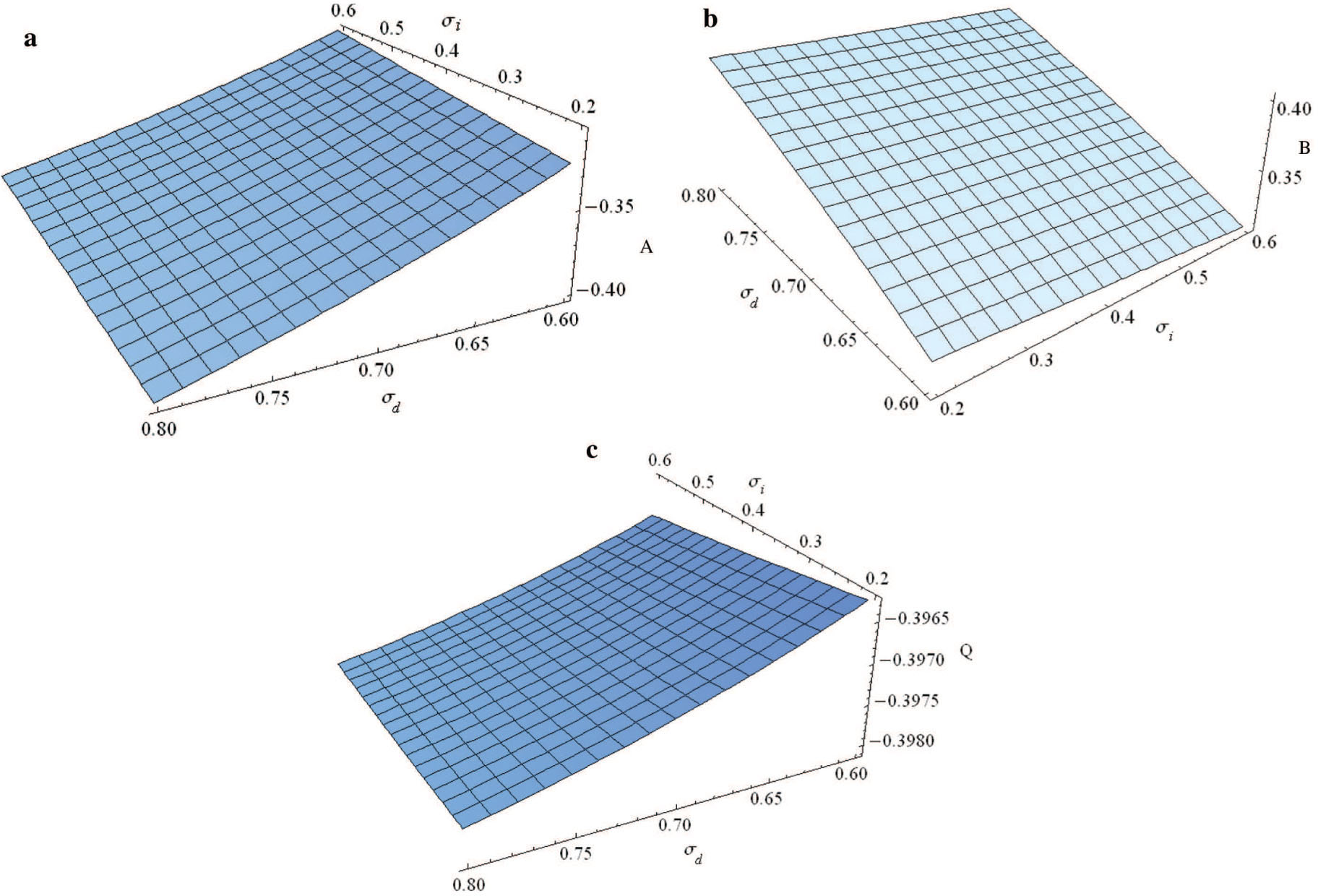
Variation of A, B, and Q with σ_i and σ_d for μ = 0.8, β = −0.5, η₁ = 0.6, η₂ = 0.8, μ₂ = 0.2, and μ₃ = 0.8.

Figure 2:

Variation of solution (31) (a) and E_f (b) with χ and β for μ₂ = 0.4, μ₃ = 0.5, ν = 0.4, σ_i = 0.2, σ_d = 0.04, η₁ = 0.2, η₂ = 0.4, and μ = 0.3.

Figure 3:

(a) Variation of solution (31) with χ and η₁ for β = −0.5, σ_i = 0.4, σ_d = 0.5, μ₂ = 0.2, μ₃ = 0.5, ν = 0.4, η₂ = 0.8, and μ = 0.8. (b) Variation of solution (31) with χ and η₂ for β = −0.5, σ_i = 0.4, σ_d = 0.7, μ₂ = 0.2, μ₃ = 0.5, ν = 0.4, η₁ = 0.4, and μ = 0.3.

Figure 4:

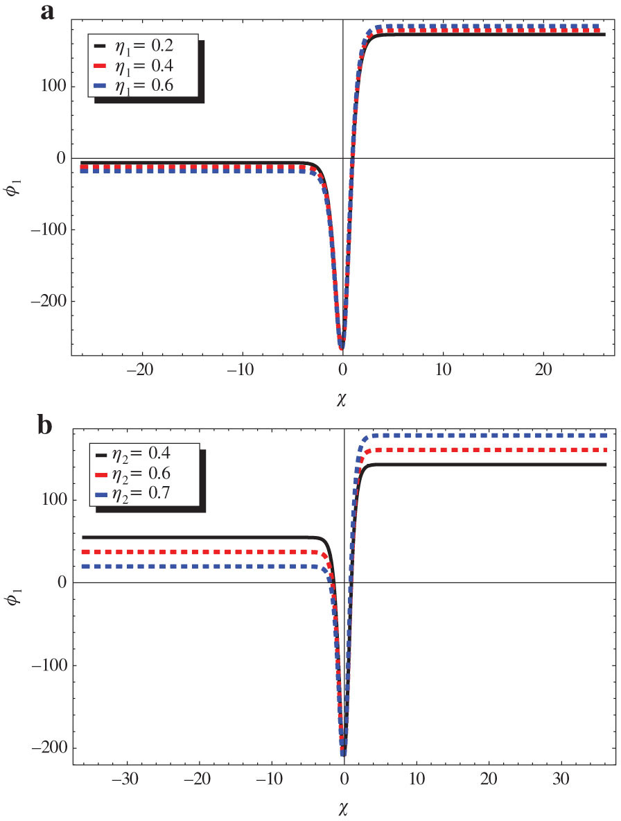
Variation of ϕ₁ (a) and E_f (b) of solution (31) with χ and β for σ_i = 0.04, σ_d = 0.5, μ₂ = 0.4, μ₃ = 0.5, ν = 0.4, η₁ = 0.2, η₂ = 0.4, and μ = 0.3 for Q ≫ B.

Figure 5:

(a) Variation of solution (31) with χ and η₁ for β = −0.5, σ_i = 0.4, σ_d = 0.5, μ₂ = 0.4, μ₃ = 0.5, ν = 0.4, η₂ = 0.8, and μ = 0.2 for Q ≫ B. (b) Variation of solution (31) with χ and η₂ for β = −0.5, σ_i = 0.4, σ_d = 0.7, μ₂ = 0.4, μ₃ = 0.5, ν = 0.4, η₁ = 0.4, and μ = 0.8 for Q ≫ B.

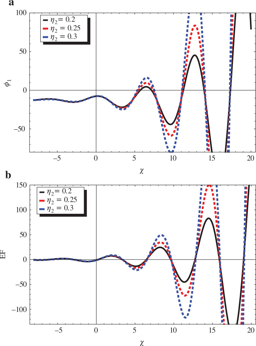
Figure 6:

Explosive profile (a) and countour plot (b) of ϕ₁ [solution (32)] with χ and η₂ for σ_i = 0.4, μ, σ_d = 0.5, β = −0.5, ν = 0.4, μ₂ = 0.4, η₁ = 0.1, and μ₃ = 0.5.

Figure 7:

Oscillatory profile of ϕ₁ (a) and E_f (b) of solution (36) with χ for σ_i = 0.4, μ, σ_d = 0.5, β = −0.5, ν = 0.4, μ₂ = 0.4, η₁ = 0.1, η₂ = 0.2, K~=5, and μ₃ = 0.5.

Figure 8:

Oscillatory profile of ϕ₁ (a) and E_f (b) of solution (36) with χ and η₂ for σ_i = 0.4, μ, σ_d = 0.5, β = −0.5, ν = 0.4, μ₂ = 0.4, η₁ = 0.1, K~=5, and μ₃ = 0.5.

Summing up, we have reported that the parameters such as temperature ratio β of free/hot ions to trapped ion and two kinematic dusty viscosity coefficient η₁, η₂ effects play an indispensable role in feature representation of electrostatic dust shock profiles in space plasma. It was important to include the spectral index of superthermal electron effect to bring our system closer to the observations. This will be taken into account in future work. Results acquired may be beneficial in understanding electrostatic shock noises in the mesosphere.

References

[1] D. A. Mendis and M. Rosenberg, Annu. Rev. Astron. Astrophys. 32, 419 (1994).10.1146/annurev.aa.32.090194.002223Search in Google Scholar
[2] A. Barkan and R. L. Merlino, Phys. Plasmas 2, 3563 (1995).10.1063/1.871121Search in Google Scholar
[3] F. Verheest, Waves in Dusty Space Plasmas, Kluwer Academic, Dordrecht 2000.10.1007/978-94-010-9945-5Search in Google Scholar
[4] P. K. Shukla and A. A. Mamun, Introduction to Dusty Plasma, Physics Institute of Physics, Bristol 2002.10.1887/075030653XSearch in Google Scholar
[5] W. M. Moslem, Phys. Scr. 65, 416 (2002).10.1238/Physica.Regular.065a00416Search in Google Scholar
[6] A. E. Mowafy, E. K. El-Shewy, and H. G. Abdelwahed, Adv. Space Res. 59, 1008 (2017).10.1016/j.asr.2016.11.009Search in Google Scholar
[7] E. C. Whipple, Rep. Prog. Phys. 44, 1197 (1981).10.1088/0034-4885/44/11/002Search in Google Scholar
[8] M. Horanyi, G. E. Morfill, and E. Grun, Nature 363, 144 (1993).10.1038/363144a0Search in Google Scholar
[9] R. L. Merlino, A. Barkan, C. Thomson, and N. D’Angelo, Phys. Plasmas 5, 1607 (1998).10.1063/1.872828Search in Google Scholar
[10] M. Horanyi and D. A. Mendis, J. Geophys. Res. 91, 355 (1986).10.1029/JA091iA01p00355Search in Google Scholar
[11] A. Mannan and A. A. Mamun, Phys. Rev. E 84, 026408 (2011).10.1103/PhysRevE.84.026408Search in Google Scholar PubMed
[12] S. A. El Wakil, M. T. Attia, M. A. Zahran, E. K. El-Shewy, and H. G. Abdelwahed, Z. Naturforsch. 61a, 316 (2006).10.1515/zna-2006-7-802Search in Google Scholar
[13] H. G. Abdelwahed, E. K. El-Shewy, M. A. Zahran, and M. T. Attia, Z. Naturforsch. 63a, 261 (2008).10.1515/zna-2008-5-605Search in Google Scholar
[14] B. Sahu and M. Tribeche, Astrophys. Space Sci. 338, 259 (2012).10.1007/s10509-011-0941-1Search in Google Scholar
[15] H. Schamel, J. Plasma Phys. 13, 139 (1975).10.1017/S0022377800025927Search in Google Scholar
[16] A. A. Mamun, Phys. Plasmas 5, 322 (1998).10.1063/1.872711Search in Google Scholar
[17] H. Schamel, N. Das, and N. Rao, Phys. Plasmas 8, 671 (2001).10.1063/1.1342027Search in Google Scholar
[18] W. S. Duan, Phys. Lett. A 317, 275 (2003).10.1016/j.physleta.2003.08.041Search in Google Scholar
[19] W. M. Moslem, W. F. El-Taibany, E. K. El-Shewy, and E. F. El-Shamy, Phys. Plasmas 12, 052318 (2005).10.1063/1.1897716Search in Google Scholar
[20] M. A. Zahran, E. K. El-Shewy, and H. G. Abdelwahed, J. Plasma Phys. 79, 859 (2013).10.1017/S0022377813000603Search in Google Scholar
[21] A. Paul, G. Mandal, A. A. Mamun, and M. R. Amin, Phys. Plasmas 20, 104505 (2013).10.1063/1.4826591Search in Google Scholar
[22] V. Pierrard and M. Lazar, Solar Phys. 267, 153 (2010).10.1007/s11207-010-9640-2Search in Google Scholar
[23] G. Livadiotis and D. J. McComas, J. Geophys. Res. 114, A11105 (2009).10.1029/2008JD010346Search in Google Scholar
[24] G. Livadiotis and D. J. McComas, J. Space Sci. Rev. 175, 183 (2013).10.1007/s11214-013-9982-9Search in Google Scholar
[25] A. M. El-Hanbaly, E. K. El-Shewy, M. Sallah, and H. F. Darweesh, Commun. Theor. Phys. 65, 606 (2016).10.1088/0253-6102/65/5/606Search in Google Scholar
[26] W. F. El-Taibany and R. Sabry, Phys. Plasmas 12, 082302 (2005).10.1063/1.1985987Search in Google Scholar
[27] E. K. El-Shewy, S. A. El-Wakil, A. M. El-Hanbaly, M. Sallah, and H. F. Darweesh, Astrophys. Space Sci., 356, 269 (2015).10.1007/s10509-014-2176-4Search in Google Scholar
[28] A. M. El-Hanbaly, E. K. El-Shewy, M. Sallah, and H. F. Darweesh, J. Theor. Appl. Phys. 9, 167 (2015).10.1007/s40094-015-0175-7Search in Google Scholar
[29] Y. Nakamura, H. Bailung, and P. K. Shukla, Phys. Rev. Lett. 83, 1602 (1999).10.1103/PhysRevLett.83.1602Search in Google Scholar
[30] E. K. El-Shewy, H. G. Abdelwahed, and M. A. Elmessary, Phys. Plasmas 18, 113702 (2011).10.1063/1.3654041Search in Google Scholar
[31] A. Sarma and Y. Nakamura, Phys. Lett. A 373, 4174 (2009).10.1016/j.physleta.2009.09.034Search in Google Scholar
[32] R. A. Cairns, R. Bingham, P. Norreys, and R. Trines, Phys. Plasmas 21, 022112 (2014).10.1063/1.4864328Search in Google Scholar
[33] H. G. Abdelwahed, Phys. Plasmas 22, 092102 (2015).10.1063/1.4929793Search in Google Scholar
[34] S. Hussain, S. Mahmood, and H. Ur-Rehman, Phys. Plasmas 20, 06210 (2013).10.1063/1.4810793Search in Google Scholar
[35] M. Shahmansouri and A. A. Mamun, Phys. Plasmas 20, 082122 (2013).10.1063/1.4818492Search in Google Scholar
[36] S. I. Popel, M. Y. Yu, and V. N. Tsytovich, Phys. Plasmas 3, 4313 (1996).10.1063/1.872048Search in Google Scholar
[37] S. I. Popel and A. A. Gisko, Nonlin. Proc. Geophys. 13, 223 (2006).10.5194/npg-13-223-2006Search in Google Scholar
[38] S. I. Popel and V. N. Tsytovich, Astrophys. Space Sci. 264, 219 (1999).10.1023/A:1002406423442Search in Google Scholar
[39] A. Rahman, A. A Mamun, and S. M. K. Alam, Astrophys. Space Sci. 315, 243 (2008).10.1007/s10509-008-9824-5Search in Google Scholar
[40] G. Mandala and P. Chatterjee, Z. Naturforsch. 65a, 85 (2010).10.1515/zna-2010-1-209Search in Google Scholar
[41] S. K. Zaghbeer, H. H. Salah, N. H. Sheta, E. K. El-Shewy, and A. Elgarayhi, J. Plasma Phys. 80, 517 (2014).10.1017/S0022377814000063Search in Google Scholar
[42] Q. Z. Luo, N. D’Angelo, and R. L. Merlino, Phys. Plasmas 6, 3455 (1999).10.1063/1.873605Search in Google Scholar
[43] S. I. Popel, T. V. Losseva, R. L. Merlino, S. N. Andreev, and A. P. Golub, Phys. Plasmas 12, 054501 (2005).10.1063/1.1885476Search in Google Scholar
[44] A. A. Mamun, B. Eliasson, and P. K. Shukla, Phys. Lett. A 332, 22 (2004).10.1016/j.physleta.2004.10.012Search in Google Scholar
[45] M. G. M. Anowar, A. Rahman, and A. A. Mamun, Phys. Plasmas 16, 053704 (2009).10.1063/1.3132630Search in Google Scholar
[46] Y. Wang, X. Guo, Y. Lu, and X. Wang, Phys. Lett. A 380, 215 (2016).10.1016/j.physleta.2015.10.005Search in Google Scholar
[47] A. S. Bains, A. Panwar, and C. M. Ryu, Astrophys. Space Sci. 360, 17 (2015).10.1007/s10509-015-2530-1Search in Google Scholar
[48] M. Michael, N. Willington, N. Jayakumar, S. Sebastian, G. Sreekala, et al., J. Theor. Appl. Phys. 10, 289 (2016).10.1007/s40094-016-0228-6Search in Google Scholar
[49] M. M. Hossen, L. Nahar, M. S. Alam, S. Sultana, and A. A. Mamun, High Energ. Dens. Phys. 24, 9 (2017).10.1016/j.hedp.2017.05.011Search in Google Scholar
[50] A. E. Dubinov, Plasma Phys. Rep. 35, 991 (2009).10.1134/S1063780X09110105Search in Google Scholar
[51] E. Saberiana, A. Esfandyari-Kalejahib, and M. Afsari-Ghazib, Plasma Phys. Rep. 43, 83 (2017).10.1134/S1063780X17010111Search in Google Scholar
[52] B. A. Klumov, S. I. Popel, and R. Bingham, JETP Lett. 72, 364 (2000).10.1134/1.1331147Search in Google Scholar
©2019 Walter de Gruyter GmbH, Berlin/Boston
Articles in the same Issue
- Frontmatter
- Atomic, Molecular & Chemical Physics
- Synthesis and Structural Investigations of Metal-Containing Nanocomposites Based on Polyethylene
- Using Stimulated Echo in Magnetic Resonance for Research of Correlation and Exchange
- Electric Spark Discharges in Water: Light Leptonic Magnetic Monopoles and Catalysis of Ordinary Beta Decays in an Extended Standard Model
- Subsonic Potentials in Ultradense Plasmas
- Dynamical Systems & Nonlinear Phenomena
- Bifurcation Analysis for Peristaltic Transport of a Power-Law Fluid