Digging into the Elusive Localised Solutions of (2+1) Dimensional sine-Gordon Equation

1 Introduction

The advent of localised solutions in terms of doubly periodic Jacobian elliptic functions [1], [2], [3] using the Painlevé Truncation Approach has completely revived the interest in the study of (2+1) dimensional integrable models and has given a filip to the identification of more general localised structures. The fact that the exponentially localised solutions called ‘dromions’ generated by Boiti et al. [4] fits into this category of solutions only as a special case has given a new dimension to the investigation of (2+1) dimensional integrable models in an effort to generate other elusive localised solutions like rogue waves, lumps etc. Rogue waves which are another interesting class of solutions, finds application in various fields [5], [6] such as hydrodynamics [7], [8], [9], [10], nonlinear optics [11], [12], [13], [14], [15], [16], [17], [18], Bose Einstein condensates [19], [20], plasma physics [21]. The important feature of rogue waves is that they come from nowhere and disappear with no trace. Lumps [22] which are algebraically localised solutions do not interact with each other. In this context, it would be interesting to revisit the (2+1) sine-Gordon equation in an attempt to extract such localised solutions in it.

2 (2+1) Dimensional sine-Gordon Equation

Konopelchenko and Rogers [23], [24] have proposed an interesting symmetric generalisation of the sine-Gordon equation to (2+1) dimensions through a reinterpretation and generalisation of a class of infinitesimal Bäcklund transformations originally introduced in gas dynamics by Loewner [25] as far back in 1952 to give the system of equations

where θ_t=ϕ+ϕ′. If we assume that ϕ′=0 and that θ_t=ϕ is independent of y, then (1, 2) becomes trivial and (1) gives the (1+1) dimensional sine-Gordon equation

Eventhough the (2+1) dimensional sine-Gordon equation has more representations, a more convenient and elegant representation is given by

where

with the characteristic variables x and y having the form

where σ²=±1 and ρ is some potential. Here σ²=1 corresponds to the sine-Gordon I equation and σ²=−1, the sine-Gordon II equation. We introduce the transformation

in (4, 5) and convert the system into a system of three coupled equations as

The (2+1) dimensional sine-Gordon equation has been investigated earlier by Radha and Lakshmanan [26] and dromion solutions have been generated. Later, Lou [27] has constructed localised solutions such as Plateau, basin, bowl and ring solitons using Variable Separation Approach. However, the nature of the collisional dynamics of dromions has not yet been understood. The question of the existence of other localised solution like lumps and rogue waves also remains open. In this paper, we utilise Truncated Painlevé Approach [1], [2], [3] to construct solutions of (2+1) sine-Gordon equation in terms of lower dimensional arbitrary functions of space and time. Expanding the physical fields q, r and the potential ρ in the form of a Laurent series in the neighbourhood of the noncharacteristic singular manifold ϕ(x, y, t)=0, (ϕ_x=ϕ_y≠0) and utilising the results of the Painlevé analysis [26], we obtain the following Bäcklund transformation by truncating at the constant level term

where q₁, r₁, ρ₁ are arbitrary solutions of the (2+1) dimensional sine-Gordon equation.

Considering the first vacuum solution given by:

we now substitute (15) with (12–14) in (9–11) to obtain the following set of equations by equating the coefficients of (ϕ⁻³, ϕ⁻³, ϕ⁻³) to obtain

Solving the above system of equations, we obtain the leading order coefficients, namely

Now, we collect the coefficients of (ϕ⁻², ϕ⁻², ϕ⁻²) to obtain

Solving the above system of equations, we obtain the following system of equations in ϕ

From the above equations, we arrive at a solution for ϕ of the form

where c is an arbitrary constant. The presence of a non-zero constant is imminent so as to avoid the occurrence of singularity in the solutions when the arbitrary functions ϕ₁, ϕ₂ → 0. Collecting the powers of (ϕ⁻¹, ϕ⁻¹, ϕ⁻¹), we have

One can easily check the compatibility of (29–31) with the (19–21) along with (28).

Collecting the coefficients of (ϕ⁰, ϕ⁰, ϕ⁰), we are left with only one equation

This is an identity.

Thus, for the choice of initial vacuum solution given by (15), the (2+1) dimensional sine-Gordon equation (9–11) has been solved through Truncated Painlevé Approach and the fields q, r, and ρ are given by

We wish to point out at this juncture that different initial solution other than the one given by (15) could lead to different solution of the (2+1) dimensional sine-Gordon equation.

3 Novel Solutions of (2+1) Dimensional sine-Gordon Equation

By choosing the arbitrary functions ϕ₁ and ϕ₂ in (33–35) in the following form, we obtain dromion solution

The plot of the (1,1) dromion for the parametric choice a=2, b=2, c=9, c₁=3, c₂=5, d₁=d₂=0, t=0 is shown in Figure 1a. It can be observed that the dromion travels with unit velocity along x direction in the x–y plane. Figure 1b shows that the potential ρ(x, y, t) is driven by a line soliton.

Figure 1:

(a) (1,1) Dromion solution, (b) the solution corresponding to the potential ρ.

3.1 More General Periodic Solutions and Multi Dromion Solutions

3.1.1 (2,1) Dromion

Next, we obtain more general dromion solution for a different choice of the arbitrary functions. As an example, we choose

(37)ϕ1=f1tanh(a1x+c1t+d1),ϕ2=f2tanh(b1y+c2t+d2)+f3tanh(b2y+c3t+d3),

where a_i, b_i, c_i, d_i and f_i are arbitrary constants.

The (2,1) dromion solution for the parametric choice a₁=2, b₁=2, b₂=3, c₁=3, c₂=5, c₃=−2, d₁=d₂=d₃=0, f₁=f₂=0.5, f₃=1, is shown in Figure 2a–c for three successive time intervals t=−2, 0 and 2. From the figures, we observe that both the taller and shorter dromions travel along the diagonals and fuse together generating a new dromion with its amplitude larger than the incident dromions. Unlike soliton interaction, they do not undergo any phase shift and exchange their amplitudes during interaction.

Figure 2:

Collisional dynamics of (2,1) dromions at (a) t=−2; (b) t=0; (c) t=2.

3.2 Dromion Pairs

3.2.1 Case (i)

If we choose ϕ₁=a₁sech²(b₁x+c₁t)+a₂sech²(b₂x+c₂t)+ a₃sech²(b₃x+c₃t), ϕ₂=1+sech²(d₁y+c₄t)+sech²(d₂y+c₅t), we can obtain six dromion pairs for the parametric choice, a₁=0.8; a₂=0.3; a₃=1.5; b₁=b₂=b₃=1; c₁=0; c₂=−0.25; c₃=0.25; c₄=0; c₅=−0.25; d₁=d₂=1 at (a) t=−55; (b) t=0; (c) t=55 as shown in Figure 3. From Figure 3, we identify three dromion pairs, moving along the diagonal direction, while three other pairs move along the x-direction. It should be noted that among the dromion pairs moving along the x-direction, the middle pair remaining stationary, while the taller pair moves from +x to −x direction and the shorter one travels in the opposite direction. One clearly observes that the three pairs interact elastically without exchanging energy.

Figure 3:

Dromion triplet pairs for the parametric choice a₁=0.8; a₂=0.3; a₃=1.5; b₁=b₂=b₃=1; c₁=0; c₂=−0.25; c₃=0.25; c₄=0; c₅=−0.25; d₁=d₂=1 at (a) t=−55; (b) t=0; (c) t=55.

3.2.2 Case (ii)

If we choose, ϕ₁=a₁sech²(b₁x+c₁t)+a₂sech²(b₂x+c₂t)+a₃ sech²(b₃x+c₃t), ϕ₂=1+sech²(d₁y+c₄t)+sech²(d₂y+c₅t), we observe a novel interaction of dromion pairs for the parametric choice, a₁=0.8; a₂=0.3; a₃=1.5; b₁=b₂=b₃=1; c₁=0.5; c₂=−0.25; c₃=0.25; c₄=0.5; c₅=−0.25; d₁=d₂=1 at (a) t=−35; (b) t=0; (c) t=35 as shown in Figure 4.

Figure 4:

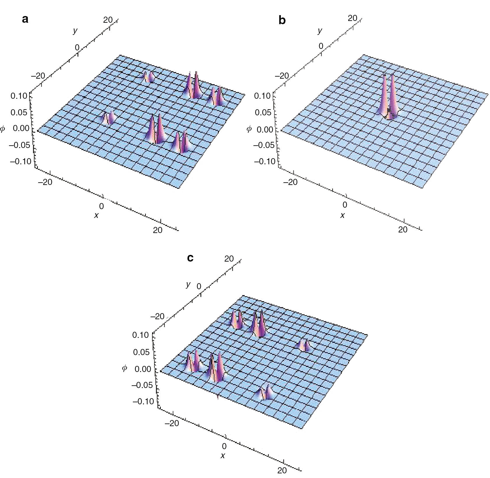
Dromion triplet pairs for the parametric choice a₁=0.8; a₂=0.3; a₃=1.5; b₁=b₂=b₃=1; c₁=0.5; c₂=−0.25; c₃=0.25; c₄=0.5; c₅=−0.25; d₁=d₂=1 at (a) t=−35; (b) t=0; (c) t=35.

In this case, we observe two important features. 1. All the dromion pairs are dynamic. 2. The three dromion pairs which were travelling along the x-direction in case (i) are now taking a diagonal path in the x–y plane.

It must be mentioned that the present dromion pairs corresponding to case (ii) have more freedom compared to the dromion triplet pairs of the Ablowitz–Kaup–Newell–Segur equation [28], which are restricted to move only along the x-direction.

Thus, in the present case, we are not only turning ON or OFF the dynamic property of dromions, but also changing its orientation in the x−y plane. As mentioned in [28], these dromion pairs are reminiscent of drones, Unmanned Aerial Vehicles employed in military, logistics etc.

3.3 Compactons

Next, we try to construct compacton solution whose interaction shows particle like behaviour. The construction of compactons bears immense significance in view of the relevance of sine-Gordon equation in the context of particle physics. To obtain compactons, we assume that the arbitrary functions are driven by piecewise functions of the form

(38)ϕ1=∑i=1N{0, kix−ωit+x0i≤−π/2bisin(kix−ωit+x0i), −π/2<kix−ωit+x0i≤π/2−2bi, kix−ωit+x0i>π/2,

(39)ϕ2=∑i=1M{0, liy+y0i≤−π/2disin(liy+y0i)−di, −π/2<liy+y0i≤π/2−2di, liy+y0i>π/2.

By choosing N=2, M=1, we get two compacton solution for the parametric choice k₁=k₂=−1, ω₁=1, ω₂=2, b₁=2, b₂=1, x₀₁=x₀₂=y₀₁=0. The time evolution of the compactons for different time intervals is shown in Figure 5. The two compactons move in the x-direction with different velocities, and they interact at t=0 and then move forward without any change in shape or velocity.

Figure 5:

The time evolution of two compacton solution at (a) t=−2; (b) t=0; (c) t=2.

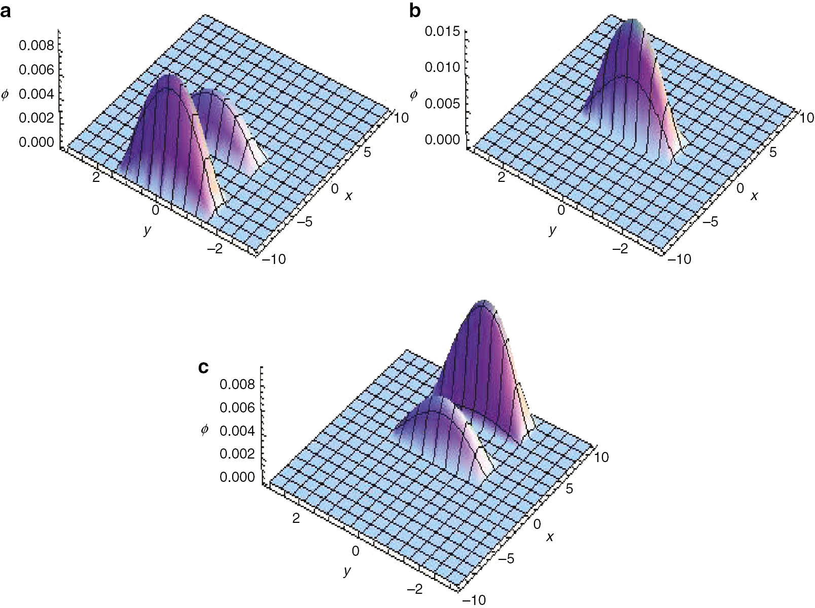
3.4 Rogue Waves

To obtain rogue waves, we assume that the arbitrary functions in the following form

(40)ϕ1=cp1t(αx2+1)2+cp2t(2(t−4)2+1)2,

(41)ϕ2=p3(y2+3)4γ2.

By choosing the following parameters choice α=0.1, β=2, γ=0.05, c=25, p₁=1, p₂=1, p₃=1, σ=1, the plot of the time evolution of the rogue wave solution is shown in Figure 6. Figure 6 underscores the unstable nature of rogue waves.

Figure 6:

The time evolution of rogue wave at (a) t=−11.7; (b) t=−11; (c) t=−10.

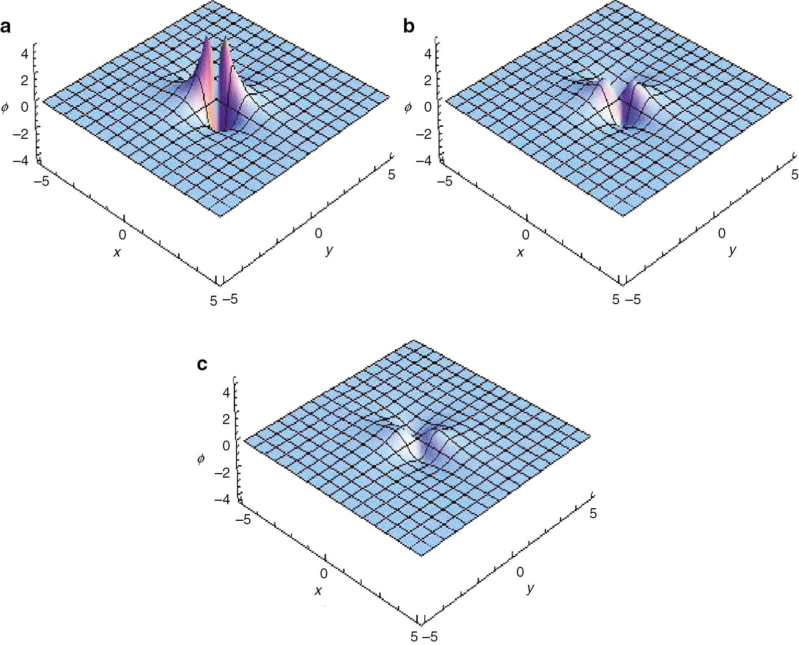
3.5 Lump Solution

To obtain lump solutions, we assume the arbitrary function in the following form

(42)ϕ1=m1((x−αt)2+1)+1,

(43)ϕ2=m2((y−βt)2+1)+1.

For the following parametric choice m₁=0.55, m₂=2, α=0.8 and β=0.4, we obtain lump solutions for different time intervals as shown in Figure 7.

Figure 7:

The time evolution of the lump solution at (a) t=−2; (b) t=0; (c) t=2.

4 Discussion

In this paper, we have considered the (2+1) dimensional sine-Gordon equation and investigated it using the Truncated Painlevé Approach to obtain its solution in closed form involving three lower dimensional arbitrary functions. We have then constructed dromions and studied their interactions. We have also studied the interaction of dromion pairs. It is shown that the dynamics of the dromion pairs can be turned ON or OFF in a desirable manner. In addition, the direction of the dromion pairs can be modified. We have also used the above analysis to construct other classes of localised solutions like compactons which remain localised over a small region of space and their associated interactions. In addition, we have also constructed rogue wave solutions and lump solutions and studied their dynamics.

References

[1] R. Radha, C. Senthil Kumar, M. Lakshmanan, X. Y. Tang, and S. Y. Lou, J. Phys. A Math. Gen. 38, 9649 (2005).10.1088/0305-4470/38/44/003Search in Google Scholar
[2] R. Radha and S. Y. Lou, Phys. Scr. 72, 432 (2005).10.1088/0031-8949/72/6/002Search in Google Scholar
[3] R. Radha, X. Y. Tang, and S. Y. Lou, Z. Naturforsch. 62a, 107 (2007).10.1515/zna-2007-3-401Search in Google Scholar
[4] M. Boiti, J. J. P. Leon, L. Martina, and F. Pempinelli, Phys. Lett. A 132, 432 (1988).10.1016/0375-9601(88)90508-7Search in Google Scholar
[5] M. Onorato, S. Residori, U. Bortolozzo, A. Montina, and F. T. Arecchi, Phys. Rep. 528, 47 (2013).10.1016/j.physrep.2013.03.001Search in Google Scholar
[6] A. Ankiewicz and N. Akhmediev, Rom. Rep. Phys. 69, 104 (2017).Search in Google Scholar
[7] A. Chabchoub, N. P. Hoffmann, and N. Akhmediev, Phys. Rev. Lett. 106, 204502 (2011).10.1103/PhysRevLett.106.204502Search in Google Scholar PubMed
[8] Q. Zhu, J. Fei, and Z. Ma, Z. Naturforsch. A 72, 795 (2017).10.1515/zna-2017-0124Search in Google Scholar
[9] Q. Zhu, Q. Wang, and Z. Zhang, Comput. Math. Math. Phys. 53, 1013 (2013).10.1134/S0965542513070191Search in Google Scholar
[10] Q. Zhu, Q. Wang, J. Fu, and Z. Zhang, J. Appl. Math. 2012, 1 (2012).10.1155/2012/252487Search in Google Scholar
[11] D. R. Solli, C. Ropers, P. Koonath, and B. Jalali, Nature 450, 1054 (2007).10.1038/nature06402Search in Google Scholar PubMed
[12] D. R. Solli, C. Ropers, and B. Jalali, Phys. Rev. Lett. 101, 233902 (2008).10.1103/PhysRevLett.101.233902Search in Google Scholar
[13] B. Kibler, J. Fatome, C. Finot, G. Millot, F. Dias, et al., Nat. Phys. 6, 790 (2010).10.1038/nphys1740Search in Google Scholar
[14] N. Akhmediev, B. Kibler, F. Baronio, M. Belić, W.-P. Zhong, et al., J. Opt. 18, 063001 (2016).10.1088/2040-8978/18/6/063001Search in Google Scholar
[15] D. Mihalache, Rom. Rep. Phys. 69, 403 (2017).10.3917/ems.larde.2016.01.0069Search in Google Scholar
[16] S. Chen, F. Baronio, J. M. Soto-Crespo, P. Grelu, and D. Mihalache, J. Phys. A Math. Theor. 50, 463001 (2017).10.1088/1751-8121/aa8f00Search in Google Scholar
[17] Y. Hu and Q. Zhu, Appl. Math. Comput. 305, 53 (2017).10.1016/j.amc.2017.01.023Search in Google Scholar
[18] Y. Hu and Q. Zhu, Nonlinear Dyn. 89, 225 (2017).10.1007/s11071-017-3448-7Search in Google Scholar
[19] Y. V. Bludov, V. V. Konotop, and N. Akhmediev, Phys. Rev. 80, 033610 (2009).10.1103/PhysRevA.80.033610Search in Google Scholar
[20] Z. Yan, V. V. Konotop, and N. Akhmediev, Phys. Rev. E 82, 036610 (2010).10.1103/PhysRevE.82.036610Search in Google Scholar
[21] H. Bailung, S. K. Sharma, and Y. Nakamura, Phys. Rev. Lett. 107, 255005 (2011).10.1103/PhysRevLett.107.255005Search in Google Scholar
[22] J. Satsuma and M. J. Ablowitz, J. Math. Phys. 20, 1496 (1979).10.1063/1.524208Search in Google Scholar
[23] B. G. Konopelchenko and C. Rogers, Phys. Lett. 158A, 391 (1991).10.1016/0375-9601(91)90680-7Search in Google Scholar
[24] B. G. Konopelchenko and C. Rogers, J. Math. Phys. 34, 214 (1993).10.1063/1.530377Search in Google Scholar
[25] C. Loewner, J. Anal. Math. 2, 219 (1952–53).10.1007/BF02825638Search in Google Scholar
[26] R. Radha and M. Lakshmanan, J. Phys. A Math. Gen. 29, 1551 (1996).10.1088/0305-4470/29/7/023Search in Google Scholar
[27] S. Y. Lou, J. Phys. A 36, 3877 (2003).10.1088/0305-4470/36/13/317Search in Google Scholar
[28] R. Radha, C. Senthil Kumar, K. Subramanian, and T. Alagesan, Comput. Math. Appl., at Press (https://doi.org/10.1016/ j.camwa.2017.12.016) (2017).Search in Google Scholar
©2018 Walter de Gruyter GmbH, Berlin/Boston
Articles in the same Issue
- Frontmatter
- Exact Solutions to Several Nonlinear Cases of Generalized Grad–Shafranov Equation for Ideal Magnetohydrodynamic Flows in Axisymmetric Domain
- A Simple Snap Oscillator with Coexisting Attractors, Its Time-Delayed Form, Physical Realization, and Communication Designs
- Nonlocal Symmetries, Conservation Laws and Interaction Solutions of the Generalised Dispersive Modified Benjamin–Bona–Mahony Equation
- A Conditionally Integrable Bi-confluent Heun Potential Involving Inverse Square Root and Centrifugal Barrier Terms