Parallel Plate Flow of a Third-Grade Fluid and a Newtonian Fluid With Variable Viscosity
-
Volkan Yıldız
 und
Yiğit Aksoy
und
Yiğit Aksoy

Abstract
Steady-state parallel plate flow of a third-grade fluid and a Newtonian fluid with temperature-dependent viscosity is considered. Approximate analytical solutions are constructed using the newly developed perturbation-iteration algorithms. Two different perturbation-iteration algorithms are used. The velocity and temperature profiles obtained by the iteration algorithms are contrasted with the numerical solutions as well as with the regular perturbation solutions. It is found that the perturbation-iteration solutions converge better to the numerical solutions than the regular perturbation solutions, in particular when the validity criteria of the regular perturbation solution are not satisfied. The new analytical approach produces promising results in solving complex fluid problems.
1 Introduction
Perturbation methods [1] have been used widely in an attempt to obtain analytical solutions for differential equations, algebraic equations, etc. However, these methods have a drawback which is the small parameter requirement and as a consequence, the solutions become only valid for weak nonlinearities. Eventually, some studies have been carried out to overcome this drawback. A few of them are the modified Lindstedt-Poincare method [2], the multiple-scales Lindstedt-Poincare method [3], the artificial parameter method [4], and the variational iteration method [5].
A different approach to obtain valid solutions for strong nonlinear systems is the iterative perturbation techniques [6–10]. In these techniques, some initial assumptions and special transformations need to be made before the iteration procedure. A new and more systematic iterative perturbation method called “the perturbation-iteration algorithm” that does not require initial assumptions and special transformations has been developed [11]. The new perturbation-iteration algorithm is based on the perturbation-iteration algorithms developed for algebraic equations [12–14]. This new iterative method has been successfully applied to Bratu-type equations [15] and some nonlinear heat transfer equations [16]. It has also been applied to Fredholm and Volterra integral equations [17] as well as to the first-order differential systems [18]. Lately, the method has been applied to strongly nonlinear vibrations [19] and to boundary-layer-type problems [20].
In this article, one of the fundamental fluid flow problem, namely the parallel plate flow, is considered. The third-grade fluid, which belongs to the Rivlin-Ericksen class, is taken as the non-Newtonian model. The model can predict the shear thinning or shear thickening behaviour as well as the normal stresses which are characteristics of a typical non-Newtonian fluid. For some previous work on the topic, see [21, 22]. Classical perturbation methods are used in the mentioned work. Hence, the solutions are valid only for a combination of the small physical parameters such as the pressure drop, non-Newtonian parameter, and the Brinkman number. For a partial list of the previous work on analytical and numerical solutions of the third-grade fluids for special flow geometries, see [23–30] for example.
In this work, the newly developed perturbation-iteration algorithm is employed to increase the range of validity of the analytical solutions. A close match between the analytical and numerical solutions can be achieved by the new method for which the classical perturbation methods yield unphysical results such as back-flow adjacent to the walls or throughout the whole domain. The perturbation-iteration algorithms are classified as PIA(n,m), n representing the number of the correction terms in the perturbation expansion and m representing the degree of the highest order derivative in the Taylor Series expansions [11–20]. Two different perturbation-iteration algorithms namely the PIA(1,1) and PIA(1,2) are employed and the results of the different algorithms are contrasted with the numerical and classical perturbation solutions. As a general rule, PIA(1,2) performs better than PIA(1,1) with exceptions.
As a second problem, a Newtonian fluid with temperature-dependent viscosity according to the Reynolds model is considered. Due to the dependence of exponentially decaying viscosity on the temperature, the governing equations become highly nonlinear and coupled. The iteration procedure enables uncoupling of the momentum and energy equations, and hence, construction of the solutions becomes easier. Results of the PIA(1,1) and the PIA(1,2) are then compared with the regular perturbation and the numerical solutions. It is found that the PIA(1,1) solutions are more reliable and straightforward due to the termination of the iterations and limitation of the logarithmic function appearing in the PIA(1,2) case.
2 Perturbation-Iteration Algorithms
An infinite number of different perturbation-iteration algorithms can be developed in theory for both algebraic and differential equations [11–20]. The algorithms were named as PIA(n,m), where n is the number of correction terms in the perturbation expansion and m is the highest order of derivative in the Taylor series expansion. n should always be less than or equal to m for the equations to be solvable. As n and m increases, the complexity of the iteration equations increases, yielding highly nonlinear coupled equations which are unsolvable analytically. Hence, it is logical to take only a few terms, and in this study, PIA(1,1) and PIA(1,2) are employed in search of analytical solutions.
2.1 Perturbation-Iteration Algorithm PIA(1,1) for Second-Order Coupled Differential Equations
The problems investigated are second-order nonlinear equations with coupling between the velocity and temperature. Hence, the theory is presented for such equations. The simplest iteration algorithm is the PIA(1,1) algorithm which is constructed by taking one correction term in the perturbation expansion and only the first-order derivate terms in the Taylor series expansion. For the general nonlinear second-order ordinary differential equations with two dependent variables
where both u and θ are functions of y, u=u(y), θ=θ(y), y being the coordinate vertical to the plates and ε is the perturbation parameter. If the equations do not possess a perturbation parameter, it can be inserted artificially. Broadly speaking, the perturbation parameter is usually inserted as a coefficient in front of the nonlinear terms. Taking just one correction term in the perturbation expansion
Substituting (3) and (4) into (1) and (2), and expanding them in a Taylor series with first-order derivatives leads to
where the total derivative is defined as
and evaluated at ε=0. Note that in this method, the dependent variables and their derivatives are considered to be independent of each other. Their contributions to the total derivative are calculated separately and added to each other as shown in (6). Using (5), one will have two coupled equations of (uc)n and (θc)n to be solved in order. With two initial guesses, u0 and θ0, which satisfy the boundary conditions, (uc)0 and (θc)0 can be calculated and later substituted into (3) and (4) to calculate u1 and θ1. This iteration procedure can be repeated until satisfactory results are obtained.
2.2 Perturbation-Iteration Algorithm PIA(1,2) for Second-Order Coupled Differential Equations
In this iteration algorithm, only one correction term in the perturbation expansion is taken and up to second-order derivatives in the Taylor series expansion are included, i.e. n=1, m=2. The algorithm is named as PIA(1,2). Again, the perturbation expansions with one correction terms
are substituted into (1) and (2) and expanded in a Taylor series up to second-order derivatives leading to
One will have two differential equations in terms of the unknowns (uc)n and (θc)n again, which have to be solved and substituted into (7) and (8). The iterative procedure is set up in the same way as explained for the PIA(1,1).
3 Parallel Plate Flow of a Third-Grade Fluid
Consider the steady-state flow of a third-grade fluid between parallel plates with heat transfer. The non-dimensional form of the equations of motion was derived by Szeri and Rajagopal [21]
where u is the dimensionless velocity, θ is the dimensionless temperature, and μ is the dimensionless viscosity. The terms are related to the dimensional (with over tilde) parameters through the following relations:
where h is the distance between the parallel plates, θ1 and θ2 are the lower and upper plate temperatures, respectively, V is the reference velocity, and μ* is the reference viscosity. The dimensionless parameters involved in (10) and (11) are
where C1 is the constant pressure drop in the axial direction, Γ is the Brinkman number, Λ is the dimensionless parameter related to the non-Newtonian behaviour, and β is the dimensional material constant which is the coefficient of the last term in the stress-constitutive relation for a third-grade fluid
where A1 and A2 are the Rivlin-Ericksen tensors [21], k is the thermal conductivity of the fluid, α1 and α2 are the material constants, and p is the pressure. The term β can be determined if the relationship between the stress and the Rivlin-Ericksen tensor of the fluid is known. The problem will be solved using the PIA(1,1) and PIA(1,2) algorithms as well as the regular perturbation method.
3.1 Perturbation-Iteration Algorithm PIA(1,1)
If the reference viscosity is selected as the Newtonian viscosity, μ=1 for the constant viscosity case. Applying the constant viscosity, (10) and (11) are rewritten in the following form:
where ε is an artificially introduced small parameter. Substituting the perturbation expansions (3) and (4) into (15) and (16), then expanding in Taylor series with first-order derivatives (5) and rearranging yields
Starting with the initial functions that satisfy the boundary conditions
and using (17), (18), (3) and (4), one will obtain the first iteration solutions as follows:
Proceeding in the same way, the subsequent iterations are
Note that the solutions are of polynomial type for this specific algorithm and becomes lengthy as the number of iterations increase.
3.2 Perturbation-Iteration Algorithm PIA(1,2)
For this case, the problem will be solved using the perturbation-iteration algorithm PIA(1,2). Substituting the perturbation expansions (7) and (8) into (15) and (16), then expanding in Taylor series up to second-order derivatives (9), the iteration formulas for the PIA(1,2) reduces to
With the initial choices
the first and the second iteration solutions are
For the sake of brevity, the lengthy solution calculated for θ2 using a symbolic manipulation program is not written here. The PIA(1,2) generated more complex solutions in functional forms as compared to the polynomial form solutions of the PIA(1,1).
3.3 Perturbation Solution
This particular problem was solved using regular perturbation methods with one correction term by Yürüsoy, Pakdemirli, and Yilbas [22]. The solutions they found under constant viscosity assumption are
It is well-known from the perturbation theory that the correction terms must be much smaller than the leading terms for the solutions to be valid. Hence, the validity criterion of these two solutions is
It should be noted that this solution is equivalent to the second iteration of PIA(1,1) when ε=1.
3.4 Comparisons With the Numerical Solution
In this section, for different values of the pressure gradient C, the non-Newtonian coefficient Λ and the Brinkman number Γ, solutions of the PIA(1,1), PIA(1,2), and the regular perturbation will be compared with each other as well as with the numerical solutions. The numerical solutions are calculated with Wolfram Mathematica’s built-in command, NDSolve.
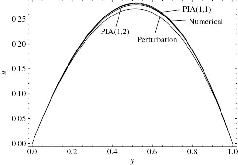
Figure 1 shows that all the solutions match well enough, when small values of the parameters satisfying the validity criterion are chosen, as expected. Especially, the non-Newtonian behaviour is assumed to be small in the calculations of Figure 1.
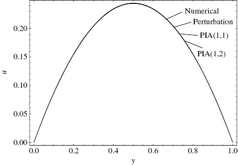
Comparison of the approximate velocity solutions with the numerical solution. ε=1, C=–2, Λ=0.025, Γ=5, Cr=0.2.
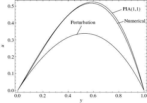
When the values of the parameters are increased further, the validity criterion does not hold anymore. The perturbation solution predicts backflow adjacent to the plates which are unphysical for a constant pressure drop between the plates (Fig. 2). The PIA(1,2) solution predicts the velocity profile better than the PIA(1,1) solution.
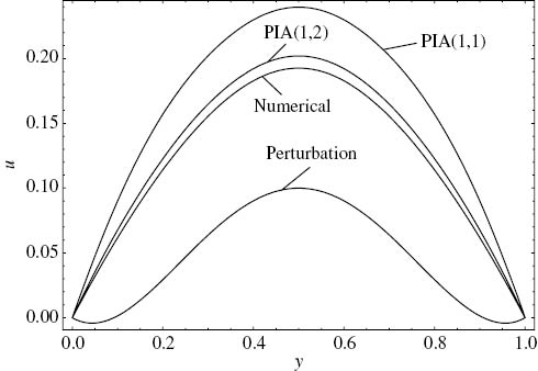
Comparison of the approximate velocity solutions with the numerical solution. ε=1, C=–2, Λ=0.6, Γ=5, Cr=4.8.
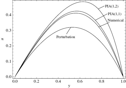
When the physical parameters are considerably larger and far beyond the validity criterion (Cr=8), the perturbation solution predicts a backflow within all the domain which is not correct at all (Fig. 3). The PIA(1,1) solution does not predict the velocity profiles quantitatively well with an exaggerated maximum velocity. The PIA(1,2) velocity profiles are in acceptable agreement with the numerical ones.
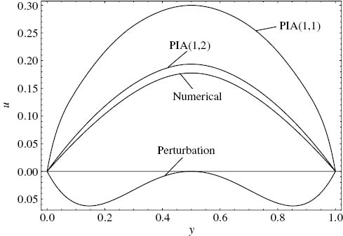
Comparison of the approximate velocity solutions with the numerical solution. ε=1, C=–2, Λ=1, Γ=5, Cr=8.
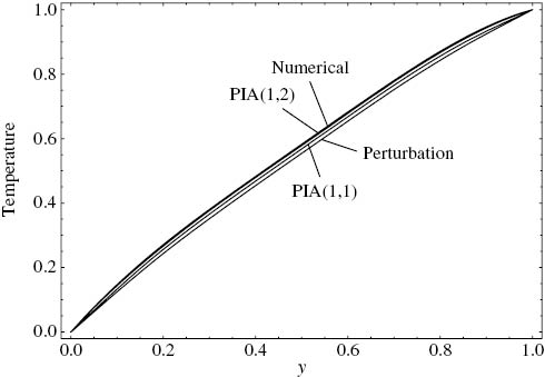
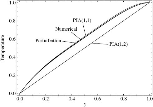
As far as the temperature profiles are considered, the matches are better among the solutions. For the criterion of 0.2, the temperatures are indistinguishable as shown in Figure 4. One reason might be that the first non-linear term involving only the Brinkman number is taken as an O(1) term in the energy equation, i.e. (11).
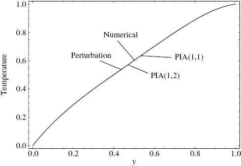
Comparison of the approximate temperature solutions with the numerical solution. ε=1, C=–2, Λ=0.025, Γ=5, Cr=0.2.
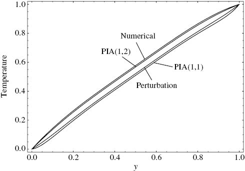
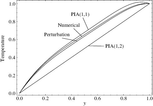
In Figure 5, the perturbation and the PIA(1,1) solutions start diverging as the criterion gets larger. PIA(1,1) seems to perform slightly better than the perturbation solution. PIA(1,2), on the other hand, agrees well with the numerical solution. Nevertheless, all the solutions are within the acceptable percentage error.
Comparison of the approximate temperature solutions with the numerical solution. ε=1, C=–2, Λ=0.6, Γ=5, Cr=4.8.
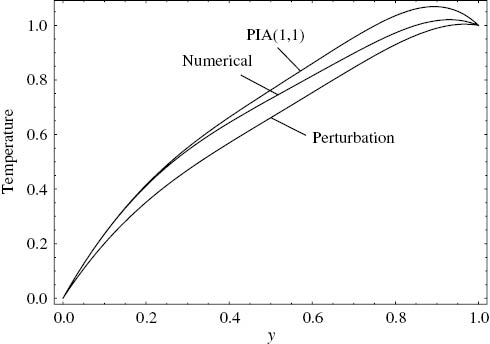
The last case for the temperature solutions are presented in Figure 6. The criterion is 8, a fairly large number compared to 1. The perturbation and the PIA(1,1) solutions diverge from the numerical solution while the PIA(1,2) solution still matches with the numerical solution reasonably. For this specific case, the perturbation solution performed slightly better than the PIA(1,1) solution.
Comparison of the approximate temperature solutions with the numerical solution. ε=1, C=–2, Λ=1, Γ=5, Cr=8.
In addition to the comparisons of the velocity and temperature profiles, the comparisons of the dimensionless shear stress and the Nusselt number are also given since these dimensionless parameters are technologically important. The dimensionless equation defining the shear stress of a third-grade fluid is
where u is the dimensionless velocity and Λ is the dimensionless parameter related to the non-Newtonian behaviour as defined before. The dimensionless shear stress is related to the dimensional one (with over tilde) as follows
Using (37), Table 1 is computed for the comparison of the shear stresses calculated by the numerical and approximate solutions for different non-Newtonian parameter values.
Comparison of the dimensionless shear stresses along the y-axis (ε=1, μ=1, C=–2, Γ=5).
| Λ | y | Numerical | PIA(1,1) | PIA(1,2) | Perturbation |
|---|---|---|---|---|---|
| 0.025 | 0 | 1.000000 | 1.000973 | 1.000279 | 0.992869 |
| 0.2 | 0.599999 | 0.600030 | 0.600009 | 0.599427 | |
| 0.4 | 0.199999 | 0.200000 | 0.200000 | 0.199998 | |
| 0.6 | –0.199999 | –0.200000 | –0.200000 | –0.199998 | |
| 0.8 | –0.599999 | –0.600030 | –0.600009 | –0.599427 | |
| 1 | –1.000000 | –1.000973 | –1.000279 | –0.992869 | |
| 0.6 | 0 | 0.999999 | 2.244493 | 1.223687 | –0.209599 |
| 0.2 | 0.599999 | 0.754888 | 0.625802 | 0.388299 | |
| 0.4 | 0.200000 | 0.200173 | 0.200049 | 0.198683 | |
| 0.6 | –0.200000 | –0.200173 | –0.200049 | –0.198683 | |
| 0.8 | –0.599999 | –0.754888 | –0.625802 | –0.388299 | |
| 1 | –0.999999 | –2.244493 | –1.223687 | 0.209599 | |
| 1 | 0 | 0.999999 | 57 | 1.443149 | –3 |
| 0.2 | 0.599999 | 1.00235 | 0.662172 | 0.177483 | |
| 0.4 | 0.200000 | 0.200733 | 0.200195 | 0.196459 | |
| 0.6 | –0.200000 | –0.200733 | –0.200195 | –0.196459 | |
| 0.8 | –0.59999 | –1.00235 | –0.662172 | –0.177483 | |
| 1 | –0.999999 | –57 | –1.443149 | 3 |
An interesting feature in the numerical results is that the shear stresses remained almost unchanged by the increase in the non-Newtonian parameter. Increasing Λ decreases the slope of the velocity due to the non-Newtonian effects and their combination in the stress equation produces similar values. However, approximate solutions give diverging results near boundaries as Λ increases. This is due to the higher slopes of the approximate solutions than the numerical ones near the boundaries as it can also be verified visually from the graphs. The shear stress decreases as y is increased till the midline where the flow reaches its maximum speed and the lowest value of shear stress is observed there. When the three approximate solutions are compared, PIA(1,2) complies best with the numerical results.
For the heat transfer, the local Nusselt number is important
where
The Nusselt number and consequently the heat transfer rate decrease as we get closer to the upper plate (Table 2). PIA(1,2) solutions are closer to the numerical ones than the other solutions. As the non-Newtonian coefficient increases, the Nusselt numbers in the lower mid-part decrease, but a slight increase is observed for the upper mid-part.
Comparison of the local Nusselt numbers along the y-axis (ε=1, μ=1, C=–2, Γ=5).
| Λ | y | Numerical | PIA(1,1) | PIA(1,2) | Perturbation |
|---|---|---|---|---|---|
| 0.6 | 0 | 1.616054 | 1.302758 | 1.554431 | 1.233333 |
| 0.2 | 1.153189 | 1.153724 | 1.151650 | 1.133340 | |
| 0.4 | 1.006492 | 1.006493 | 1.006492 | 1.006475 | |
| 0.6 | 0.993508 | 0.993507 | 0.993508 | 0.993525 | |
| 0.8 | 0.846811 | 0.846276 | 0.848349 | 0.866656 | |
| 1 | 0.383946 | 0.697242 | 0.445569 | 0.766667 | |
| 1 | 0 | 1.562657 | 0.177323 | 1.415282 | 0.833333 |
| 0.2 | 1.143772 | 1.132576 | 1.138883 | 1.102239 | |
| 0.4 | 1.006391 | 1.006395 | 1.006391 | 1.006346 | |
| 0.6 | 0.993609 | 0.993605 | 0.993609 | 0.993653 | |
| 0.8 | 0.856228 | 0.867424 | 0.861117 | 0.897769 | |
| 1 | 0.437343 | 1.822677 | 0.584718 | 1.166667 |
In conclusion, for the velocity profiles, all solutions are in reasonable agreement within the range of validity of the perturbation solution. Beyond the range of validity, the PIA solutions agree better with the numerical ones and the PIA(1,2) performs better than the PIA(1,1). The perturbation solution, however, is not reliable as it gives quantitatively and qualitatively wrong behaviour for velocities if the criterion is not satisfied. For the temperature profiles, the qualitative behaviour is the same for all solutions although there are some small variations in the results quantitatively. For temperature profiles, the best agreement is observed for PIA(1,2). In conclusion, for non-Newtonian fluids, the perturbation iteration algorithms may be used to find approximate analytical solutions at least for some simple flow geometries.
4 Parallel Plate Flow of a Newtonian Fluid With Temperature-Dependent Viscosity
Although the fluid model is Newtonian and simpler in this case, the dependence of the viscosity on the temperature introduces further nonlinearities and makes the momentum and energy equations coupled. The steady-state equations and the boundary conditions are
where u is the dimensionless velocity, θ is the dimensionless temperature, and μ is the dimensionless viscosity. The dimensionless parameters are defined in terms of the dimensional ones as
where h is the distance between the parallel plates, θ1 and θ2 are the temperatures of the bottom and top plates, respectively, V is the reference velocity, and μ* is the reference viscosity. The dimensionless physical parameters are
where C1 is the constant pressure drop in the axial direction, C is the dimensionless pressure drop parameter, and Γ is the Brinkman number. For this problem, the viscosity is an exponentially decaying function of the temperature
which is called the Reynolds model. For m=0, μ=1 and the model reduces to the constant viscosity case. ε is introduced artificially in the coefficient of the nonlinear term in the energy equation and also as a coefficient in front of the viscosity decay parameter. It can be taken as 1 at the end of the calculations.
4.1 Perturbation-Iteration Algorithm PIA(1,1)
Substituting the Reynolds model viscosity into the problem, (40) and (41) are rewritten in the following form:
One correction term perturbation expansions are substituted into (45) and (46) and then expanded in Taylor series with first-order derivatives. The following equations of iteration are obtained as a result
Simple initial functions that satisfy the boundary conditions can be selected as
The first iteration solutions are then
Finally, the second and third iteration solutions are calculated
Note again that the PIA(1,1) solutions are of polynomial type.
4.2 Perturbation-Iteration Algorithm PIA(1,2)
The iteration equations of PIA(1,2) are found by first substituting the perturbation expansions with one correction terms into (40) and (41) and then expanding in Taylor series up to second-order derivatives
Starting with the same initial guesses as in the previous section
the first iteration solutions are found as
From the definition of the logarithm, εm<1 must hold for the first iteration solutions to be valid. The next iteration is not calculated due to this limited validity of the solution and the complexities encountered in the equations.
4.3 Perturbation Solution
For the regular perturbation solution of the problem, expansions with two correction terms are taken into account
Reynolds model of viscosity is also expanded in a series
Substituting these expansions into (40) and (41) and separating at each order of approximation, one will have three sets of equations to be solved consecutively both for the velocity and temperature profiles. The equations at each order are solved and the solutions are substituted into the perturbation expansions. Thus, the two term perturbation solutions for the problem are
Imposing the condition that each correction term be much smaller than the previous term, the validity criteria are
The first criterion involves the viscosity decaying parameter and the second criterion involves a combination of the pressure drop as well as the Brinkman number.
4.4 Comparisons With the Numerical Solution
In this section, solutions of the PIA(1,1), PIA(1,2), and the regular perturbation will be compared with each other as well as with the numerical solutions for different values of the pressure drop, the viscosity parameter, and the Brinkman number. The numerical solutions are calculated with Wolfram Mathematica’s built-in command, NDSolve.
In Figure 7, the PIA(1,1) and the PIA(1,2) solutions are in good agreement with the numerical solution, while there is a small discrepancy for the perturbation solution especially at the fully developed flow region. Despite the fact that only the first criterion is satisfied, the perturbation solution does not introduce much error.
Comparison of the approximate velocity solutions with the numerical solution. ε=1, m=0.2, C=–2, Γ=5, Cr1=0.13, Cr2=3.33.
In Figure 8, due to the increase in the viscosity parameter, the curves bent to the right and the maximum velocities occur closer to the upper plate where the temperature is greater compared to the lower one. The closest approximate solution to the numerical one is the PIA(1,1) solution. Since m is large and the PIA(1,2) solution consists of a logarithmic function for which εm<1 condition must hold, the solution over-predicts the location and magnitude of the maximum velocity.
Comparison of the approximate velocity solutions with the numerical solution. ε=1, m=0.8, C=–2, Γ=5, Cr1=0.53, Cr2=3.33.
Figure 9 shows the comparison of the approximate solutions for m=1.1. Only the PIA(1,1) and the perturbation solutions are plotted here, as this is an undefined region for the PIA(1,2) solution. The perturbation solution under-predicts the location and magnitude of the maximum velocity. However, PIA(1,1) solution still remains close to the numerical one.
Comparison of the approximate velocity solutions with the numerical solution. ε=1, m=1.1, C=–2, Γ=5, Cr1=0.73, Cr2=3.33.
Regarding the temperature profiles, the PIA(1,1) and the perturbation solution matches well with the numerical solution in the case where one of the criteria is not satisfied (Fig. 10). On the other hand, the first iteration solution of PIA(1,2) being θ1=y is a rough estimation and differs from the others.
Comparison of the approximate temperature solutions with the numerical solution. ε=1, m=0.2, C=–2, Γ=5, Cr1=0.13, Cr2=3.33.
When the viscosity parameter m is increased, it is observed from Figure 11 that the solutions begin diverging. Here, the perturbation solution performed relatively better than PIA(1,1) especially in the region near the upper plate.
Comparison of the approximate temperature solutions with the numerical solution. ε=1, m=0.6, C=–2, Γ=5, Cr1=0.4, Cr2=3.33.
The last case where m=1.1 is presented in Figure 12. Both criterion are higher than should be for a regular solution, and hence, the perturbation solution is further away from the numerical solution when compared with PIA(1,1) which agrees quite well up to y=0.4 and gradually diverges as y increases.
Comparison of the approximate temperature solutions with the numerical solution. ε=1, m=1.1, C=–2, Γ=5, Cr1=0.73, Cr2=3.33.
Similar to the previous problem, the shear stresses and the Nusselt numbers of the flow along the y-axis will be contrasted. The dimensionless shear stress equation of the steady-state parallel plate flow of a Newtonian fluid is
with the dimensionless parameters defined in (12) and (38). Substituting the Reynolds model of viscosity into (69), the shear stress equation takes the below form
In Table 3, the shear stress values slightly increase as m gets larger. When the approximate results are compared, with few exceptions, the shear stress values calculated by PIA(1,1) comply better to the numerically calculated ones than the other methods.
Comparison of the shear stresses along the y-axis (ε=1, C=–2, Γ=5).
| m | y | Numerical | PIA(1,1) | PIA(1,2) | Perturbation |
|---|---|---|---|---|---|
| 0.2 | 0 | 1.032986 | 1.036508 | 1.037159 | 1.033333 |
| 0.2 | 0.632987 | 0.634332 | 0.637684 | 0.606880 | |
| 0.4 | 0.232987 | 0.235495 | 0.237963 | 0.218159 | |
| 0.6 | –0.167013 | –0.164612 | –0.164121 | –0.163940 | |
| 0.8 | –0.567013 | –0.567986 | –0.570977 | –0.542711 | |
| 1 | –0.967013 | –0.979878 | –0.985384 | –0.944269 | |
| 0.8 | 0 | 1.124712 | 1.184127 | 1.257330 | 1.133333 |
| 0.2 | 0.724712 | 0.723869 | 0.869724 | 0.578785 | |
| 0.4 | 0.324712 | 0.333863 | 0.488367 | 0.210891 | |
| 0.6 | –0.075288 | –0.056265 | 0.068221 | –0.103451 | |
| 0.8 | –0.475288 | –0.463573 | –0.501909 | –0.369055 | |
| 1 | –0.875288 | –0.965701 | –1.66852 | –0.653025 |
The Nusselt number for the steady-state parallel plate flow of a Newtonian fluid with temperature-dependent viscosity is defined as
where
Comparison of the local Nusselt numbers along the y-axis (ε=1, C=–2, Γ=5).
| M | y | Numerical | PIA(1,1) | Perturbation |
|---|---|---|---|---|
| 0.2 | 0 | 1.939028 | 1.961667 | 1.922222 |
| 0.2 | 1.211579 | 1.230780 | 1.204622 | |
| 0.4 | 0.994709 | 1.008970 | 0.995289 | |
| 0.6 | 0.978488 | 0.991812 | 0.980622 | |
| 0.8 | 0.803331 | 0.793469 | 0.808622 | |
| 1 | 0.072784 | –0.059444 | 0.088889 | |
| 0.6 | 0 | 2.201195 | 2.255000 | 2.100000 |
| 0.2 | 1.301565 | 1.354886 | 1.253867 | |
| 0.4 | 0.966530 | 1.017268 | 0.972533 | |
| 0.6 | 0.934261 | 0.985506 | 0.955199 | |
| 0.8 | 0.755545 | 0.731087 | 0.785867 | |
| 1 | 0.163626 | –0.601667 | –0.066667 | |
| 1.1 | 0 | 2.684067 | 2.690417 | 2.322222 |
| 0.2 | 1.504344 | 1.552292 | 1.315422 | |
| 0.4 | 0.922851 | 1.034557 | 0.944089 | |
| 0.6 | 0.837894 | 0.971505 | 0.923422 | |
| 0.8 | 0.644476 | 0.635637 | 0.757422 | |
| 1 | –0.627251 | –1.448194 | –0.261111 |
In Table 4, it is shown that increasing m has increased the Nusselt number in the region near the lower plate while decreasing it near the upper plate. When the Nusselt number is tracked along the y-axis for a fixed m value, it seems to decrease as we get close to the upper plate. In the table, PIA(1,2) is not presented as its first iteration solution is a rough estimation and the second iteration cannot be calculated due to a singularity in the velocity profile. When the other two approximate solutions are compared, both produce reasonable approximations to the numerical data with few exceptions.
Consequently, for the velocity profiles, all solutions agree well with each other when the validity criteria are satisfied. Exceeding the limit of the criteria, solutions start to diverge with perturbation solution inheriting too much error. In addition to that PIA(1,2) solutions agree well for the small values of the viscosity parameter m; however, they diverge due to the criterion caused by the logarithmic function as m gets larger. In general, the PIA(1,1) gives the most reliable results for the velocity profiles for the case of Newtonian flow. Calculating PIA(1,1) up to third iteration may be the significant cause, while due to limitations, PIA(1,2) algorithm is terminated at the first iteration. For the temperature profiles, PIA(1,1) and the perturbation solutions give similar results. If the criteria are too large, then the perturbation solution ceases to be valid.
The solutions of the previous section and this section can only be contrasted for the limiting cases of Λ=0 when the non-Newtonian parameter vanishes. Both PIA(1,1) and PIA(1,2) solutions given in (25) and (33) reduce to
For (33), when Λ approaches zero, the singularity should be removed by the L’Hopital’s rule. The above solution can also be retrieved for the Newtonian fluid with Reynolds model parameter m=0. For m=0 in (55) and (66), (72) is obtained.
5 Conclusions
In this study, the perturbation-iteration algorithms are applied to the flow of a third-grade fluid and to the flow of a Newtonian fluid with temperature-dependent viscosity. Two different perturbation-iteration algorithms are used. Results are then compared with the regular perturbation and the numerical solutions. The following conclusions can be made.
The perturbation-iteration algorithm solutions are better in terms of predicting the velocity profiles for the case of third-grade fluid flow. The regular perturbation solutions predict erroneous velocity profiles such as unphysical backflow when the validity criteria are not met.
In determining the temperature profiles in a third-grade fluid, the variations among the solutions are marginal and even the regular perturbation solutions predict the temperatures with acceptable errors beyond the validity criteria.
For the Newtonian flow with variable viscosity, the most reliable velocity and temperature profiles correspond to the PIA(1,1) solutions. PIA(1,2) did not produce better solutions than those of PIA(1,1) due to the termination of the iterations and due to the limitations of the logarithmic function. The regular perturbation solutions are better than the PIA(1,2) solutions especially in predicting the temperature profiles.
The perturbation-iteration algorithms in general produce acceptable results beyond the limits of the validity range of the regular perturbation solutions.
PIA(1,2) solutions are of functional type while PIA(1,1) solutions are of polynomial type.
Especially, for non-Newtonian fluids, analytical solutions are rare. It is shown that the perturbation iteration method is effective in constructing analytical solutions to complex fluid problems.
References
[1] A. H. Nayfeh, Introduction to Perturbation Techniques, John Wiley and Sons, New York 1981.Suche in Google Scholar
[2] H. Hu, J. Sound Vib. 269, 409 (2004).10.1016/S0022-460X(03)00318-3Suche in Google Scholar
[3] M. Pakdemirli, M. M. F. Karahan, and H. Boyacı, Math. Comput. Appl. 14, 31 (2009).10.3390/mca14010031Suche in Google Scholar
[4] J. I. Ramos, Appl. Math. Comput. 193, 303 (2007).10.1016/j.amc.2007.03.050Suche in Google Scholar
[5] A. M. Wazwaz, Commun. Nonlinear Sci. Numer. Simulat. 16, 3881 (2011).10.1016/j.cnsns.2011.02.026Suche in Google Scholar
[6] V. Marinca and N. Herisanu, Acta Mech. 184, 231 (2006).10.1007/s00707-006-0336-5Suche in Google Scholar
[7] H. Hu, J. Sound Vib. 298, 1159 (2006).10.1016/j.jsv.2006.06.005Suche in Google Scholar
[8] J. H. He, J. Sound Vib. 7, 631 (2001).Suche in Google Scholar
[9] H. Hu, J. Sound Vib. 298, 446 (2006).10.1016/j.jsv.2006.05.023Suche in Google Scholar
[10] D. D. Ganji, S. Karimpour, and S. S. Ganji, Int. J. Mod. Phys. B 23, 2469 (2009).10.1142/S0217979209052406Suche in Google Scholar
[11] M. Pakdemirli, Y. Aksoy, and H. Boyacı, Math. Comput. Appl. 16, 890 (2011).10.3390/mca16040890Suche in Google Scholar
[12] M. Pakdemirli and H. Boyacı, Appl. Math. Comput. 184, 783 (2007).10.1016/j.amc.2006.05.207Suche in Google Scholar
[13] M. Pakdemirli, H. Boyacı, and H. A. Yurtsever, Math. Comput. Appl. 12, 117 (2007).10.3390/mca12020117Suche in Google Scholar
[14] M. Pakdemirli, H. Boyacı, and H. A. Yurtsever, Math. Comput. Appl. 13, 123 (2008).10.3390/mca13020123Suche in Google Scholar
[15] Y. Aksoy and M. Pakdemirli, Comput. Math. Appl. 59, 2802 (2010).10.1016/j.camwa.2010.01.050Suche in Google Scholar
[16] Y. Aksoy and M. Pakdemirli, Int. J. Numer. Meth. H. 22, 814 (2012).10.1108/09615531211255725Suche in Google Scholar
[17] İ. Dolapci, M. Şenol, and M. Pakdemirli, J. Appl. Math. 2013, 1 (2013).10.1155/2013/682537Suche in Google Scholar
[18] M. Şenol, İ. Dolapci, Y. Aksoy, and M. Pakdemirli, Abstr. Appl. Anal. 2013, 1 (2013).10.1155/2013/704137Suche in Google Scholar
[19] M. Pakdemirli, J. Vib. Control (2015), in press.Suche in Google Scholar
[20] M. Pakdemirli, SpringerPlus 5, 208 (2016). Doi: 10.1186/s40064-016-1859-4.10.1186/s40064-016-1859-4Suche in Google Scholar
[21] A. Z. Szeri and K. R. Rajagopal, Int. J. Nonlinear Mech. 20, 91 (1985).10.1016/0020-7462(85)90003-4Suche in Google Scholar
[22] M. Yürüsoy, M. Pakdemirli, and B. S. Yılbaş, J. Mech. Eng. Sci. 222(4), 653 (2008).10.1243/09544062JMES872Suche in Google Scholar
[23] M. Ayub, A. Rasheed, and T. Hayat, Int. J. Eng. Sci. 41, 2091 (2003).10.1016/S0020-7225(03)00207-6Suche in Google Scholar
[24] M. Massoudi and I. Christie, Int. J. Non-Linear Mech. 30, 687 (1995).10.1016/0020-7462(95)00031-ISuche in Google Scholar
[25] T. Hayat, A. H. Kara, and E. Momoniat, Int. J. Non-Linear Mech. 38, 1533 (2003).10.1016/S0020-7462(02)00116-6Suche in Google Scholar
[26] R. Ellahi, M. Raza, and K. Vafai, Math. Comput. Model 55, 1876 (2012).10.1016/j.mcm.2011.11.043Suche in Google Scholar
[27] T. Hayat and A. H. Kara, Math. Comput. Model 43, 132 (2006).10.1016/j.mcm.2004.12.009Suche in Google Scholar
[28] O. A. Bég, M. J. Uddin, M. M. Rashidi, and N. Kavyani, J. Eng. Thermophys. 23(2), 79 (2014).10.1134/S1810232814020015Suche in Google Scholar
[29] M. M. Rashidi, M. T. Rastegari, M. Asadi, and O. Anwar Bég, Chem. Eng. Commun. 199, 231 (2012).10.1080/00986445.2011.586756Suche in Google Scholar
[30] M. Keimanesh, M. M. Rashidi, Ali J. Chamkha, and R. Jafari, Comput. Math. Appl. 62, 2871 (2011).10.1016/j.camwa.2011.07.054Suche in Google Scholar
©2016 by De Gruyter
Artikel in diesem Heft
- Frontmatter
- Decay Mode Solutions for the Supersymmetric Cylindrical KdV Equation
- Cooling of Moving Wavy Surface through MHD Nanofluid
- Parallel Plate Flow of a Third-Grade Fluid and a Newtonian Fluid With Variable Viscosity
- Flow of a Micropolar Fluid Through a Channel with Small Boundary Perturbation
- Exact Solutions for Stokes’ Flow of a Non-Newtonian Nanofluid Model: A Lie Similarity Approach
- A New Reduction of the Self-Dual Yang–Mills Equations and its Applications
- Quasi-periodic Solutions to the K(−2, −2) Hierarchy
- Superposition of Solitons with Arbitrary Parameters for Higher-order Equations
- Elastic and Thermal Properties of Silicon Compounds from First-Principles Calculations
- Exact Solutions for N-Coupled Nonlinear Schrödinger Equations With Variable Coefficients
- Rapid Communication
- Electrical Conductivity of Molten CdCl2 at Temperatures as High as 1474 K