Soret and Dufour Effects in the Flow of Williamson Fluid over an Unsteady Stretching Surface with Thermal Radiation

1 Introduction

The flow induced by a stretching surface with heat transfer is prominent in several engineering processes such as aerodynamic extrusion of plastic sheets, annealing and tinning of copper wire, crystal growing, food processing, paper production, and glass blowing. The end product in such applications greatly depends upon the stretching and cooling rates at the surface. Also the fluids involved mostly in such processes are non-Newtonian. The well-known Navier–Stokes equations are inadequate for the flow analysis of non-Newtonian fluids. Different from viscous fluids, constitutive equations for the description of many rheological properties of non-Newtonian fluids have been suggested (see [1–9]). Further, the combined effects of heat and mass transfer have an important role in the fields such as distribution of temperature and moisture over agricultural fields and groves of fruit trees (crops damage due to freezing, fog formation, and dispersion), cooling towers and food processing. There is no doubt that the driving potentials become intricate in nature when heat and mass transfer occur simultaneously between the fluxes. Obviously both temperature and composition gradients can generate the energy flux. The energy flux due to the composition/temperature gradient is known as the Dufour/Soret effect. The Dufour and Soret effects in general are of small order of magnitude than the effects through Fourier’s or Fick’s laws and are often neglected in heat and mass transfer processes. The Soret or thermal diffusion effect is utilized for isotope separation and a mixture of light molecular weight gases (hydrogen–helium) and of medium molecular weight gases (nitrogen–air); the Dufour effect was found to be of a magnitude such that it cannot be neglected. In recent years, progress has been considerably made for the Soret and Dufour effects in the boundary layer flows (see [10–19]).

In the past, much attention was paid to the heat transfer analysis in the boundary layer flows either through the prescribed surface temperature or through the prescribed heat flux. Recently a convective boundary condition for the heat transfer effect in such flow has been employed by Aziz [20]. Patil et al. [21] analysed the influence of the convective condition along with mass transfer for two-dimensional double diffusive mixed convection. Ramesh and Gireesha [22] employed a numerical method to solve mathematical formulation resulting from the flow of Maxwell fluid with the convective boundary condition. Rashad et al. [23] studied mixed convection boundary layer flow by taking into account the thermal convective condition. Hayat et al. [24] carried out an analysis to examine nanofluid flow near a stretched surface with the convective boundary condition. Hamad et al. [25] investigated heat and mass transfer together with the thermal convective condition. Makinde and Aziz [26] presented a numerical solution of the heat and mass transfer of nanofluid from a horizontal plate with the convective boundary condition. Hayat et al. [27] examined forced convection resulting from the three-dimensional flow of Jeffrey fluid with a convectively heated plate. Das et al. [28] concentrates on the boundary layer flow of nanofluid over a heated stretching sheet with the convective boundary condition. Hayat et al. [29] discussed convective conditions for heat transfer in Maxwell fluid.

Motivated by the above-referenced works, it is of paramount interest in this investigation to examine the effects of heat and mass transfer convective conditions, Soret and Dufour, thermal radiation, and viscous dissipation on the boundary layer flow of Williamson fluid over an unsteady stretching surface. None of the above attempts simultaneously analysed all such effects even in viscous fluid/steady flow over a stretching surface. The momentum, energy, and concentration equations are transformed into a set of ordinary differential systems and then solved implementing the homotopy analysis method (HAM) [30–34]. To reveal the tendency of solutions, the results for velocity, temperature, and concentration are graphically displayed. The local Nusselt number, Sherwood number, and skin friction coefficient are analysed through tabulated values. This paper is organized as follows. Section 2 contains problem formulation. In Section 3, we present the solutions. The convergence of the obtained solutions is presented in Section 4. Sections 5 and 6 consist of discussion and conclusion, respectively.

2 Problem Formulation

Consider a two-dimensional flow of an incompressible Williamson fluid over an unsteady stretching sheet with heat and mass transfer. The horizontal sheet is placed at y= 0 and the flow is confined in the region y>0. The sheet is stretched by two equal and opposite forces. The effects of Soret and Dufour, thermal radiation, and viscous dissipation are considered. Further, we take the convective boundary condition for both temperature and concentration fields.

The velocity, temperature, and concentration fields subject to the boundary layer and Rosseland approximations are governed by the following equations:

(1)∂u∂x + ∂v∂y = 0, (1)

(2)∂u∂t + u∂u∂x + v∂u∂y = ν(∂2u∂y2 + 2Γ∂u∂y∂2u∂y2), (2)

(3)∂T∂t + u∂T∂x + v∂T∂y = α∗∂2T∂y2 − 1ρcp∂qr∂y  + μ0ρcp[(∂u∂y)2 + Γ(∂u∂y)3] + DmkTcpcs∂2C∂y2, (3)

(4)∂C∂t + u∂C∂x + v∂C∂y = Dm∂2C∂y2 + DmkTTm∂2T∂y2, (4)

(5)u = Uw(x), v = 0, − k∂T∂y = h(Tf − T), − Dm∂C∂y = km(Cf − C) at  y = 0,u → 0, T → T∞, C → C∞ as y → ∞, (5)

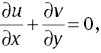
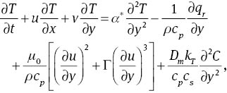
where u and v represent the velocity components along the x- and y-directions, respectively, Γ>0 is the characteristic time, Uw(x,t) = cx(1 − at) is the stretching velocity of the sheet, u_∞ (where a and c are positive constants), ν = μ0ρ is the kinematic viscosity, T is the fluid temperature, T_∞ is the ambient fluid temperature, C is the fluid concentration, C_∞ is the ambient fluid concentration, α^* is the thermal diffusivity, k is the thermal conductivity, c_p is the specific heat, qr = −16σT∞33k∗∂T∂y is the radiative heat flux, k^* is the mean absorption coefficient, σ is the Stefan–Boltzmann constant, c_s is the concentration susceptibility, D_m is the molecular diffusivity of the species concentration, k_T is the thermal diffusion ratio, h is the wall heat transfer coefficient, k_m is the wall mass transfer coefficient, T_m is the mean fluid temperature, and the convective heating process is characterised by temperature T_f and associated concentration near the surface is C_f.

The appropriate transformations are defined as follows:

(6)u = cx(1 − at)f′(η), v = −cν(1 − at)f(η),θ(η) = T − T∞Tf − T∞, ϕ(η) = C − C∞Cf − C∞, η = cν(1 − at)y. (6)

With the help of the above transformations, (1) is identically satisfied and (2)–(5) yield

(7)f‴ + f f″ − f′2 − A(f′ + η2f″) + 2λf″ f‴ = 0, (7)

(8)(1 + 43R)θ″ + Pr(fθ′ − Aη2θ′) + Pr Duϕ″  + Pr Ec(f″2 + λf″3) = 0, (8)

(9)ϕ″ + ScSr θ″ + Sc(fϕ′ − Aη2ϕ′)= 0. (9)

(10)f = 0, f′ = 1, θ′(0) = − Bi1(1 − θ(0)), ϕ′(0)= −Bi2(1 − ϕ(0)) at η = 0,f′ = 0, θ = 0, ϕ = 0 at η = ∞, (10)

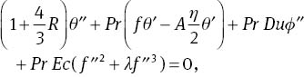
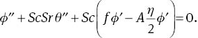
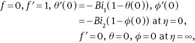
where A is the unsteadiness parameter, λ is the Williamson fluid parameter, Pr is the Prandtl number, Du is the Dufour number, Sr is the Soret number, Sc is the Schmidt number, Ec is the Eckert number, Bi₁ is the thermal Biot number, Bi₂ is the concentration Biot number, and R is the radiation parameter. The definitions of these parameters are

A = ac,λ = Γxc3ν(1 − at)3,Du = DmkT(Cf − C∞)νcρcs(Tf − T∞),Pr = να∗,Sr = DmkT(Tf − T∞)νTm(Cf − C∞),Ec = Uw2(x)cp(Tf − T∞),Sc = νDm,Bi1 = hkν(1 − at)c,R = 4σT∞3kk∗,Bi2 = kmDmν(1 − at)c.

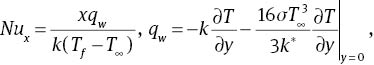
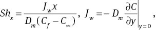
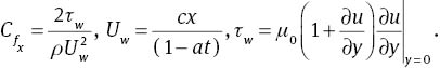
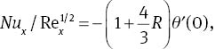
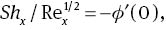
The local Nusselt number Nu_x, local Sherwood number Sh_x, and skin friction coefficient Cfx are defined by

(11)Nux = xqwk(Tf − T∞), qw = −k∂T∂y − 16σT∞33k∗∂T∂y|y = 0, (11)

(12)Shx = JwxDm(Cf − C∞),  Jw = − Dm∂C∂y|y = 0, (12)

(13)Cfx = 2τwρUw2, Uw = cx(1 − at), τw = μ0(1 + ∂u∂y)∂u∂y|y = 0. (13)

The dimensionless forms of (11)–(13) are

(14)Nux/Rex1/2 = − (1 + 43R)θ′(0), (14)

(15)Shx/Rex1/2 = −ϕ′(0), (15)

(16)12CfxRex1/2 = (f″(0) + λf″2(0)). (16)

Rex = Uw(x,t)xν is the local Reynolds number.

3 Series Solutions

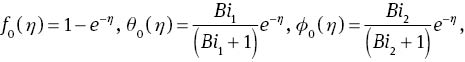
The initial approximations and auxiliary linear operators for the series solutions are chosen as follows:

(17)f0(η) = 1 − e−η, θ0(η) = Bi1(Bi1 + 1)e−η, ϕ0(η) = Bi2(Bi2 + 1)e−η, (17)

(18)ℒf = f‴ − f′, ℒθ = θ″ − θ, ℒθ = ϕ″ − ϕ, (18)

with

(19)ℒf(C1 + C2eη + C3e− η) = 0, (19)

(20)ℒθ(C4eη + C5e− η) = 0, (20)

(21)ℒϕ(C6eη + C7e−η) = 0, (21)

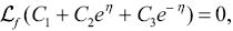
in which C_i (i= 1–7) are the arbitrary constants. If p∈ [0 1] denotes an embedding parameter, and ℏ_f,ℏ_θ, and ℏ_φ are the non-zero auxiliary parameters, then the zeroth-order deformation problems can be put into the forms

(22)(1 − p) ℒf [f^(η;p) − f0(η)] = pℏfNf [f^(η;p)], (22)

(23)(1 − p) ℒθ [θ^(η;p)−θ0(η)] = pℏθNθ [f^(η;p),θ^(η;p),ϕ^(η;p)], (23)

(24)(1−p) ℒϕ [ϕ^(η;p) − ϕ0(η)] = pℏϕNϕ [f^(η;p),θ^(η;p),ϕ^(η;p)], (24)

(25)f^(0;p) = 0, f^′(0;p) = 1, f^′(∞;p) = 0, θ^′(0;p) = −Bi1[1 − θ^(0;p)],ϕ^'(0;p) = −Bi2[1 − ϕ^(0;p)], θ^(∞;p) = 0, ϕ^(∞;p) = 0, (25)

(26)Nf[f^(η;p)] = ∂3f^(η,p)∂η3 + f^(η,p)∂2f^(η,p)∂η2 − (∂f^(η,p)∂η)2− A(∂f^(η,p)∂η + η2∂2f^(η,p)∂η2) + 2λ∂2f^(η,p)∂η2∂3f^(η,p)∂η3. (26)

(27)Nθ[θ^(η;p),f^(η;p),ϕ^(η;p)] = (1 + 43R)∂2θ^(η,p)∂η2 + Pr f^(η,p)∂θ^(η,p)∂η−Pr Aη2∂θ^(η,p)∂η + Pr Du∂2ϕ^(η,p)∂η2+Pr Ec[(∂2f^(η,p)∂η2)2 + λ(∂2f^(η,p)∂η2)3]. (27)

(28)Nϕ[ϕ^(η;p),θ^(η;p),f^(η;p)] = ∂2ϕ^(η,p)∂η2 + Sc f^(η,p)∂ϕ^(η,p)∂η− ScAη2∂ϕ^(η,p)∂η + Sc Sr∂2θ^(η,p)∂η2. (28)

For p= 0 and p= 1, we have

(29)f^(η;0) = f0(η), θ^(η;0) = θ0(η), ϕ^(η;0) = ϕ0(η)f^(η;1) = f(η), θ^(η;1) = θ(η), ϕ^(η;1) = ϕ(η) (29)

and when p moves from 0 to 1, then f(η, p), θ(η, p), and ϕ(η, p) approach f₀(η), θ₀(η), and ϕ₀(η) to f(η), θ(η), and ϕ(η). Now f, θ, and ϕ in Taylor’s series can be written as follows:

(30)f(η,p) = f0(η) + ∑m = 1∞fm(η)pm, (30)

(31)θ(η,p) = θ0(η) + ∑m = 1∞θm(η)pm, (31)

(32)ϕ(η,p) = ϕ0(η) + ∑m = 1∞ϕm(η)pm, (32)

(33)fm(η) = 1m!∂mf(η;p)∂ηm|p = 0, θm(η) = 1m!∂mθ(η;p)∂ηm|p = 0, ϕm(η) = 1m!∂mϕ(η;p)∂ηm|p = 0. (33)

Note that the convergence depends upon ℏ_f, ℏ_θ, and ℏ_φ. By proper choices of ℏ_f, ℏ_θ, and ℏ_φ, the series (30)–(32) converge for p= 1 and hence

(34)f(η) = f0(η) + ∑m = 1∞fm(η), (34)

(35)θ(η) = θ0(η) + ∑m = 1∞θm(η), (35)

(36)ϕ(η) = ϕ0(η) + ∑m = 1∞ϕm(η). (36)

The mth-order deformation problems are given by

(37)ℒf[fm(η) − χmfm − 1(η)] = ℏfℛfm(η), (37)

(38)ℒθ[θm(η) − χmθm − 1(η)] = ℏθℛθm(η), (38)

(39)ℒϕ[ϕm(η) − χmϕm − 1(η)] = ℏϕℛϕm(η), (39)

(40)fm(0) = f′m(0) = f′m(∞) = 0,   θ′m(0) − Bi1θm(0) = θm(∞) = 0,ϕ′m(0) − Bi2ϕm(0) = ϕm(∞) = 0, (40)

(41)ℛfm(η) = f‴m − 1 + ∑k = 0m − 1[fm − 1 − kf″k − f′m − 1 − kf′k] −A(f′m − 1 + η2f″m − 1.) + 2λ∑k = 0m − 1f″m − 1 − kf‴k, (41)

(42)ℛθm(η) = (1 + 43R)θ″m−1 + Pr(∑k = 0m − 1θ′m − 1 − kfk − Aη2θ′m − 1)+ Pr Ec[∑k = 0m − 1f″m − 1 − kf″k  + λ∑k = 0m(∑l = 0kf″l f″k − l)f″m − k]+ Pr Duϕ″m − 1, (42)

(43)ℛϕm(η) = ϕ″m − 1 + Sc Srθ″m − 1 + Sc(∑k = 0m − 1ϕ′m − 1 − kfk − Aη2ϕ′m − 1), (43)

(44)χm = {0, m ≤ 1,1, m > 1. (44)

The general solutions of (37)–(39) are given by

(45)fm(η) = fm∗(η) + C1 + C2eη + C3e−η, (45)

(46)θm(η) = θm∗(η) + C4eη + C5e− η, (46)

(47)ϕm(η) = ϕm∗(η) + C6eη + C7e− η, (47)

in which fm∗,θm∗, and ϕm∗ denote the particular solutions and the constants C_i (i= 1–7) are determined from boundary conditions (41), i.e.,

C2 = C4 = C6 = 0, C3 = ∂f∗(η)∂η|η = 0,           C1 = − C3 − f∗(0),C5 = 1Bi1 + 1[∂θ∗(η)∂η|η = 0 − Bi1θ∗(0)],C7 = 1Bi2 + 1[∂ϕ∗(η)∂η|η = 0 − Bi2ϕ∗(0)].

4 Convergence Analysis

The convergence of series solutions depends upon the involved non-zero auxiliary parameters. To check the convergence of series solutions, we plot the ℏ-curves for the velocity, temperature, and concentration fields. Figure 1 depicts the ℏ-curves of f″(0), θ′(0), and ϕ′(0) for different values of physical parameters involved in the problem. The admissible value of ℏ_f is –1.6<ℏ_f<–0.3, for ℏ_θ it is –1.8<ℏ_θ<–0.3, and for ℏ_φ it is –1.8<ℏ_φ<–0.2. It is clearly seen from these figures that the series solutions converge in the whole region of η when ℏ_f= –1.1, ℏ_θ= –1.5, and ℏ_φ= –1.4. ℏ-curves for the residual error are plotted in Figure 2. Figure 2 may be considered as counter-check to Figure 1 in order to confirm their convergence analysis. The square residual errors are defined as

Figure 1:

ℏ-curves for f″(0), θ′(0), and ϕ′(0).

Figure 2:

Residual error for f″(0), θ′(0), and ϕ′(0).

(48)Δmf = ∫01[ℛfm(η,ℏf)]2dη,Δmθ = ∫01[ℛθm(η,ℏθ)]2dη,Δmϕ = ∫01[ℛϕm(η,ℏϕ)]2dη. (48)

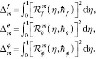
Table 1 shows the convergence of series solutions for different orders of approximations. It is obvious from this table that the 25^th order of approximations is sufficient for the convergent series solutions.

5 Results and Discussion

In this section, the effects of different parameters on the velocity, temperature, and concentration fields have been analysed. Figure 3 shows the influence of the unsteadiness parameter A on the velocity profile. An increase in the unsteadiness parameter A decreases the stretching rate c, which in turn reduces the velocity and momentum boundary layer. Opposite behaviour of concentration and temperature fields is observed for the unsteadiness parameter A (see Figs. 4 and 5). The influence of the Williamson fluid parameter λ on the velocity field is displayed in Figure 6. The velocity is found to decrease when λ is increased. Physically, it is true because an increase in relaxation time causes higher resistance to the fluid flow which ultimately reduces the velocity field. This higher resistance also enhances the collisions in the fluid that increases the temperature field (see Fig. 7). Figure 8 demonstrates the increasing behaviour of the concentration field for larger values of λ. Figures 9 and 10 depict that the thermal and concentration Biot numbers have an increasing impact on the temperature and concentration fields, respectively. Larger values of the thermal and concentration Biot numbers enhance the temperature gradient and thermal boundary layer thickness. Soret and Dufour effects on the temperature and concentration profiles are shown in Figures 11 and 12, respectively. The values of the Soret and Dufour numbers are chosen in such a way that their product is constant provided that the mean temperature T_m is kept constant as well. With an increase of the Dufour number (i.e., a decrease of the Soret number) the temperature difference between hot and surrounding fluid decreases, which in result enhances the temperature and thermal boundary layer thickness. Further, the intermolecular forces become weak and, as a result, the concentration decreases. The larger Prandtl number has a relatively lower thermal diffusivity. The influence of the Eckert number Ec on the temperature θ(η) is sketched in Figure 13. The viscous dissipation effect increases with an increase in the Eckert number. Therefore, a significant increase in the temperature and thermal boundary layer thickness is noticed. Figure 14 illustrates the concentration profiles for different values of the Schmidt number. The increase in Sc means lower molecular diffusivity, which results in the reduction of the concentration boundary layer.

Figure 3:

Influence of A on f′(η).

Figure 4:

Influence of A on θ(η).

Figure 5:

Influence of A on ϕ(η).

Figure 6:

Influence of λ on f′(η).

Figure 7:

Influence of λ on θ(η).

Figure 8:

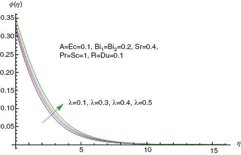
Influence of λ on ϕ(η).

Figure 9:

Influence of Bi₁ on θ(η) and θ′(η)

Figure 10:

Influence of Bi₂ on ϕ(η) and ϕ′(η).

Figure 11:

Influences of Du and sron θ (η).

Figure 12:

Influences of Du and Sr on ϕ(η).

Figure 13:

Influence of Ec on θ(η).

Figure 14:

Influence of Sc on ϕ(η).

Tables 2 analyses the variations of different physical parameters with the local Nusselt number. The local Nusselt number increases with an increase in Pr, R, and Bi₁. A slight variation in the local Nusselt number is noticed by increasing the values of the Soret number Sr. It is observed that an increase in A, λ, Bi₂, Ec, Du, and Sc leads to a decrease in the heat transfer rate at the surface. Table 3 presents the numerical values of the local Sherwood number for different values of physical parameters. It is observed that the mass transfer coefficient in terms of the local Sherwood number increases with an increase in Sc, Du, and Bi₂, while an increase in A, λ, Sr, and Bi₁ leads to a decrease in the value of the local Sherwood number. Table 4 shows the effects of various parameters on the skin friction coefficient. The skin friction coefficient is negative for all physical parameters. Physically, negative values of the skin friction coefficient means that the surface exerts a drag force on the fluid. The magnitude of the skin friction coefficient is increased by increasing the values of A and λ. Table 5 depicts the comparison of the skin friction coefficient from the previous study. From this table we found excellent argument.

6 Conclusions

Salient features of convective heat and mass transfer in the flow of Williamson fluid over an unsteady stretching sheet are investigated in the presence of Soret and Dufour effects. The main outcomes of the present attempt can be mentioned as follows.

• The velocity field f′(η) and momentum boundary layer thickness are decreasing functions of A and λ.

• The behaviours of concentration and temperature fields corresponding to A and λ are qualitatively similar.

• The influences of the radiation parameter R and Eckert number Ec on the temperature field are reverse to that of Pr.

• The effects of Soret and Dufour numbers on the temperature and concentration fields are quite opposite.

• The Prandtl number Pr and Eckert number Ec have dual behaviour on the concentration field.

• Concentration field decays most rapidly for larger values of the Schmidt number Sc.

• Effects of thermal and concentration Biot numbers on the temperature and concentration fields are qualitatively similar.

References

[1] K. Das, Int. J. Heat Mass Tran. 54, 3505 (2011).Suche in Google Scholar
[2] T. Hayat, A. Safdar, M. Awais, and Awatif A. Hendi, Z. Naturforsch. 66a, 635 (2011).10.5560/zna.2011-0032Suche in Google Scholar
[3] T. Hayat, M. Awais, and S. Obaidat, J. Heat Transfer 134, 044503 (2012).10.1115/1.4006032Suche in Google Scholar
[4] M. Awais, A. Alsaedi, and T. Hayat, Int. J. Numer. Math. Heat Fluid Flow 24, 483 (2014).10.1108/HFF-04-2012-0084Suche in Google Scholar
[5] R. Ellahi, S. U. Rahman, M. Mudassar Gulzar, S. Nadeem, and K. Vafai, Appl. Math. Inf. Sci. 8, 1567 (2014).Suche in Google Scholar
[6] M. Turkyilmazoglu, and I. Pop, Int. J. Heat Mass Tran. 57, 82 (2013).Suche in Google Scholar
[7] M. M. Rashidi, M. Ali, N. Freidoonimehr, B. Rostami, and A. Hossian, Adv. Mech. Eng. 2014, 735939 (2014).Suche in Google Scholar
[8] M. Sheikholeslami, H. R. Ashorynejad, D. D. Ganji, and M. M. Rashidi, Commun. Numer. Anal. 2014, 00166 (2014).Suche in Google Scholar
[9] T. Hayat, H. Yasmin, and M. Al-Yami, Comput. Fluids 89, 242 (2014).10.1016/j.compfluid.2013.10.038Suche in Google Scholar
[10] S. Shateyi, S. S. Motsa, and P. Sibanda, Math. Prob. Eng. 2010, 627475 (2010).Suche in Google Scholar
[11] T. Hayat, S. A. Shehzad, and A. Alsaedi, Appl. Math. Mech. (Engl. Ed.) 33, 1301 (2012).10.1007/s10483-012-1623-6Suche in Google Scholar
[12] F. E. Alsaadi, S. A. Shehzad, T. Hayat, and S. J. Monaquel, J. Mech. 29, 623 (2013).Suche in Google Scholar
[13] T. Hayat, R. Naz, S. Asghar, and A. Alsaedi, Int. J. Numer. Methods Heat Fluid Flow 24, 498 (2014).10.1108/HFF-03-2012-0076Suche in Google Scholar
[14] T. Hayat, M. Mustafa, and S. Obaidat, ASME J. Fluids Eng. 133, 021202 (2011).Suche in Google Scholar
[15] C. Hsiao, W. Chang, M. Char, and B. Tai, Appl. Math. Comput. 244, 390 (2014).Suche in Google Scholar
[16] S. Wang, and W. Tan, Int. J. Heat Fluid Flow 32, 88 (2011).10.1016/j.ijheatfluidflow.2010.10.005Suche in Google Scholar
[17] M. Turkyilmazoglu, and I. Pop, Int. J. Heat Mass Tran. 55, 7635 (2012).Suche in Google Scholar
[18] M. M. Rashidi, T. Hayat, E. Erfani, S. A. M. Pour, and A. A. Hendi, Commun. Nonlin. Sci. Numer. Simul. 16, 4303 (2011).Suche in Google Scholar
[19] A. Zaib, and S. Shafie, J. Franklin Inst. 351, 1268 (2014).Suche in Google Scholar
[20] A. Aziz, Commun. Nonlin. Sci. Numer. Simul. 14, 1064 (2009).Suche in Google Scholar
[21] P. M. Patil, E. Momoniat, and S. Roy, Int. J. Heat Mass Tran. 70, 313 (2014).Suche in Google Scholar
[22] G. K. Ramesh, and B. J. Gireesha, Ain Shams Eng. J. (2014) (in press).Suche in Google Scholar
[23] A. M. Rashad, A. J. Chamkha, and M. Modather, Comput. Fluids 86, 380 (2013).10.1016/j.compfluid.2013.07.030Suche in Google Scholar
[24] A. Alsaedi, M. Awais, and T. Hayat, Commun. Nonlin. Sci. Numer. Simul. 17, 4210 (2012).Suche in Google Scholar
[25] M. A. A. Hamad, Md. J. Uddin, and A. I. Md. Ismail, Int. J. Heat Mass Tran. 55, 1355 (2012).Suche in Google Scholar
[26] O. D. Makinde, and A. Aziz, Int. J. Ther. Sci. 50, 1326 (2011).Suche in Google Scholar
[27] S. A. Shehzad, A. Alsaedi, and T. Hayat, Int. J. Heat Mass Tran. 55, 3971 (2012).Suche in Google Scholar
[28] K. Das, P. R. Duari, and P. K. Kundu, J. Egypt. Math. Soc. (2014) (in press).Suche in Google Scholar
[29] T. Hayat, Z. Iqbal, M. Mustafa, and A. Alsaedi, Nucl. Eng. Des. 252, 242 (2012).Suche in Google Scholar
[30] S. Liao, Commun. Nonlin. Sci. Numer. Simul. 15, 2003 (2010).Suche in Google Scholar
[31] T. Hayat, S. Asad, and A. Alsaedi, Appl. Math. Mech. (Engl. Ed.) 35, 1 (2014).10.1007/s10483-014-1824-6Suche in Google Scholar
[32] T. Hayat, S. Asad, M. Mustafa, and Hamed H. Alsulami, Chin. Phys. B 23, 084701 (2014).10.1088/1674-1056/23/8/084701Suche in Google Scholar
[33] M. M. Rashidi, B. Rostami, N. Freidoonimehr, and S. Abbasbandy, Ain Shams Eng. J. 5, 901 (2014).Suche in Google Scholar
[34] M. Sheikholeslami, R. Ellahi, H. R. Ashorynejad, G. Domairry, and T. Hayat, J. Comput. Theor. Nanosci. 11, 486 (2014).Suche in Google Scholar
[35] S. Sharidan, T. Mahood, and I. Pop, Int. J. Appl. Mech. Eng. 11, 647 (2006).Suche in Google Scholar
©2015 by De Gruyter
Artikel in diesem Heft
- Frontmatter
- Editorial
- Content matters – the new face of ZNA
- Original Communications
- Nonreciprocal Optical Tunnelling Through Evanescently Coupled Tamm States in Magnetophotonic Crystals
- The Wronskian Solution and Soliton Resonance of the Nonisospectral Generalised Sawada–Kotera Equation
- A Mathematical Study for Three-Dimensional Boundary Layer Flow of Jeffrey Nanofluid